1. INTRODUCTION
Our experiences in teaching the basics of celestial navigation, in a classroom-bound setting have been frustrating. There appears to be a lack of contemporary and easily adaptable visual models for illustrating the basic ideas involved. Our needs are to cover a unit on navigation, in a general education university course (Astronomy and Astrophysics, 2008), but also note a wider need for the continued importance of teaching celestial navigation (Prudente, Reference Prudente2015). Part of our effort is to take the classical celestial navigational techniques, and develop a contemporary and somewhat general set of visuals that can appeal to today's university student.
In the lessons presented here, we start by placing a “lost” ship at some location in the ocean, and challenge the students to think how they might find its location. At this point in our class, the students are versed in the history and challenges of navigation, beginning with the “longitude problem” of the 1700s, and are aware of using Polaris and/or the Sun (at noon) to find latitude, as well as the “dual chronometer” technique to find longitude.
Our goals in teaching celestial navigation are as follows. At the onset, students are open to the idea that objects “in the sky” can be used for navigation purposes (i.e. the north star, southern cross, etc.). However, they tend to believe that use of a sextant is merely an “old fashioned” version of a Global Positioning System (GPS) unit, both of which readily return the latitude and longitude of one's position. We start by demonstrating how a sextant only measures the altitude (angle) of a celestial object, ultimately giving one's distance from the Geographical Position (GP) of the object. (In this work, the Sun is exclusively used.)
This is followed by a tour of (both modern and historical) navigational tables that show how knowing the GP of the Sun in advance is possible, after a “reminder” about seasons on Earth. We establish that the Sun's GP is well known and tabulated, and has been for hundreds of years. From the sextant reading, the idea of a circle of position is illustrated, and how a simple compass reading (and some common sense) allows one to immediately eliminate most of the circle as a possible location of the ship. The work presented in this paper was motivated by our need to easily show how a GP, ship and circle of position are all linked on a map, using some form of media that is highly visual and easily adaptable in real-time (even during a classroom discussion); thus, the use of Google Maps.
Proceeding with our lesson, we assume that the ship is stationary and wait for the GP of the Sun to move with time, allowing for the determination of a second circle of position. We then highlight the intersection points of the two circles. Issues of scale are discussed, as is the lack of importance of seeing both the GP and the ship on the same map. Through this approach, we can convince the students of the iterative nature of celestial navigation, in that one takes repeated sights of the Sun, while monitoring the section of the ocean where intersection points of the circles of position seem to be collecting. The goal of our lesson is to allow the students to gain some familiarity with the “sight-reduction” procedure that follows a sextant reading, and that a GPS-style “you are here, now” result is not necessarily the outcome. Instead, we show how repeated measurements give more and more confidence in where one thinks one is located, that ultimately can only be verified by comparison with an established landmark.
As mentioned, our lessons rely only on the sequential sights of the Sun, with a somewhat contrived scenario, including times of the day and year, that will maximise the chances of navigational success. This includes the availability of several sequential altitude measurements of the Sun, between 10° and 70° (Schlereth, Reference Schlereth2000), conveniently scaled maps, drawing tools, and easy computation involving basic spherical trigonometry. All of these have been sources of frustration in our teaching efforts.
We have dispensed with much however, in favour of a mapping tool everyone is familiar with: Google Maps (Google Maps, 2015). It is the intent of this paper to introduce teachers of celestial navigation to the utility of Google Maps in developing their lesson. We also believe the work here would be of interest to those with an interest in celestial navigation, who wish to test and simulate the sight-reduction procedure, from sextant reading to position plotting. The Google Map technique allows for the quick production of accurate, flexible and highly visual teaching aids, which we have found very useful in our teaching efforts.
This paper is organised as follows. After demonstrating the use of Google Maps from a programming standpoint, the ramifications of the Assumed Position (AP) are analysed. In particular, we present an analysis of the proximity of the initial AP to the actual position of the ship, and the outcome of a sight-reduction based on it.
2. WORKING WITH GOOGLE MAPS
Our route to using Google Maps for celestial navigation must extend beyond the point-and-click interface. We wish to programmatically control a map to aid in considerations of celestial navigation. The work presented here discusses using Google Maps as driven by Javascript, a language built into all web-browsers. Thus, the only software tool needed here is a web browser, running on a computer connected to the Internet.
We begin by simply displaying a familiar Google Map under Javascript control. In order to do this, one must request a (free) “developer key” from Google (Google Key, 2014). Once done, a basic map can be created with the following Javascript code:
<!DOCTYPE html>
<html>
<head>
<title>Celestial navigation using Google Maps</title>
<script
src="https://maps.googleapis.com/maps/api/js?key=API_
KEY&callback=init_map&libraries=geometry"
async defer></script>
</head>
<body>
<div id="map" style="width:800px; height:800px;"></div>
<script>
function init_map()
{
map = new google.maps.Map(document.getElementById(’map’),
{
center: {lat: 32, lng: -120},
zoom: 3,
scaleControl: true
});
//start
//end
}
</script>
</body>
</html>
This code should be typed into a text editor, saved as an.html file (such as celnav.html), then loaded directly into a web-browser using the “File→Open...” menu. Note the string “API_KEY” should be replaced by your developer key. All of our code is available by contacting the author.
This will show a map with a zoom level of three, centred about the point (32N, 120W). We note the function init_map() is called when the Google Map library has been loaded and is ready, in the <script src=...> line. Despite the over-use of opening and closing grouping symbols typical of Javascript, we hope the core structure on how the centre latitude and longitude of the map's view is set, as well as the zoom level, is clear. The scaleControl: true directive places a small scale indicator in the lower right corner of the map, which provides a useful verification for any distances that may arise (this indicator will be in kilometres, needing a division by 1·852 to convert to Nautical Miles (NM)).
We note that throughout the usage of these maps, the usual mouse controls are always available, including panning and zooming as needed by the lesson. As we proceed, the reader is instructed to add code blocks as discussed, starting immediately after the //start line, and before the //end line.
3. THE LESSON: FINDING A LOST SHIP USING SIGHTS OF THE SUN
In this lesson, we will place a “lost” ship at a latitude of 27°20·0′N, and a longitude of 160°49·0′W, and assume the ship is stationary, and will remain at this position for many hours.Footnote 1 Of course, if we were actually navigating, we would not know these coordinates, but it is the aim of the lesson here to demonstrate how to narrow in on them. When on this lost ship, a hypothetical watch gives us the time of 21:20 GMT on 5 April 2015, and a virtual sextant reading (NOAA, 2015) yields the altitude of the Sun to be 60·63° (corrected for atmospheric refraction, at zero dip, to the Sun's centre). A look in the Nautical Almanac (Nautical Almanac, 2015) for this date and time to reveals the GP of the Sun to have a declination of 6°12·2′ North, with a Greenwich Hour Angle (GHA) of 139°20·1′.
We note two issues here. The first is in the mixture of our numbers. Classical celestial navigation uses the degrees and arc-minutes convention, but with our computational approach, decimals are a better fit. In our teaching, we discuss both forms of the numbers, but move rather quickly to the decimal representation, as they are less of a distraction to the students, as we focus on the larger ideas of celestial navigation. Second, it is beyond the scope of our class (mostly due to time constraints) to discuss the details of obtaining a proper sextant reading. We briefly discuss the various corrections, and students are typically quick to ask about weather considerations, which helps us to further compare and contrast classical celestial navigation from the use of a GPS receiver.
We now follow the St. Hilaire sight-reduction plan from Schlereth (Reference Schlereth2000), Karl (Reference Karl2011), and Bowditch (NIMA, 2015).
3.1. Preliminaries
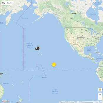
To begin our lesson, we immediately plot the ship and the GP of the Sun, as shown in Figure 1.
A GP and hypothetical lost ship, plotted programmatically, using Javascript and Google Maps.

Adding our first code blocks to the lines above, both the ship and Sun can be plotted on the map via this code (added immediately after the //start line and before the //end line above)
gha = −(139+20/60);
decl= 6+12.2/60;
ship_lat = 27+20/60;
ship_lng = −(160+49/60);
new google.maps.Marker({
map: map,
position: {lat: ship_lat, lng: ship_lng},
icon: {url: ’images/ship_tr.png’,
size: new google.maps.Size(50,32),
orgin: new google.maps.Point(25,16),
anchor: new google.maps.Point(25,16)}
});
new google.maps.Marker({
map: map,
position: {lat: decl, lng: gha},
icon: {url: ’images/sun.png’,
size: new google.maps.Size(50,50),
orgin: new google.maps.Point(25,25),
anchor: new google.maps.Point(25,25)},
});
Here we define variables involving the GP of the Sun and the location of the lost ship. Markers are placed on the map using the google.maps.Marker construct. We note each marker must be told on which map it is to be placed (via the map: map declaration), with the variable map referencing the active Google map. We then give the icon a position in the form of a latitude (lat) and longitude (lng). In the absence of the icon: line, a familiar red balloon will appear. Here we have used images of a ship and the Sun to increase the visual appeal. These images are to be placed in a folder called images, relative to the location where celnav.html is saved, and will render a small ship and Sun on our map as shown in Figure 1, by instructing the Marker construct to use the images in the icon directive. The size, origin, and anchor tags are used to centre the icons at the given latitude and longitude point, and may need to be adjusted, depending on browser nuances, or the exact icon one uses (stated settings are for Safari 10.1). We sized all icons to be 50x50 pixels.
We immediately begin to see the visualisation power of this Google Maps approach. The position of the ship is clear, as is the meaning of the GP of the Sun, and already we are in a realm of extreme numerical precision, able to circumvent our previous teaching modes that included sketches on the blackboard or contrived freehand computer drawings.
Next, based on the altitude of the Sun, we plot our Circle Of Position (COP), which can be handled using the google.maps.Circle method in Google Maps, or
alt = 60.63;
coalt = 90 − alt;
cop_path = new google.maps.Circle({
geodesic: true,
strokeColor: ’#FF0000’,
strokeOpacity: 1.0,
strokeWeight: 2,
center: {lat: decl, lng: gha},
radius: 111120 * coalt,
fillOpacity: 0.0
});
cop_path.setMap(map);
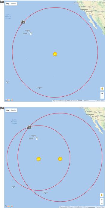
Here we define variables to hold both the altitude and co-altitude (Karl, Reference Karl2011) of the Sun. Next, we call the google.maps.Circle method using the declination and GHA as its centre, and a radius of the co-altitude (converted to metres, as required). This method is ideal for this application, as such circles are computed to be a “spherical cap” of the points of the Earth's sphere. The result is shown in Figure 2(a).
(a) A circle of position for our lost ship, relative to the Sun. (b) Two circles of position for our lost ship.

Plotting another COP using the Sun's GP one hour later (6°13·2′N,154°20·0′W) with an altitude of 68·0°, results in Figure 2(b), which shows both COPs intersecting at the ship's position.
This is a gratifying check of our tools, and a critical link between the GP of the Sun and its observed altitude from the ship. It leads naturally to a discussion on the mechanical mapping problems of having both the ship and GP on the same map (i.e. the ship icon is as large as some states in the continental United States), and in eliminating one of the intersection points of the COPs, owing to their large radius. If done using actual times during a class, students can be asked to study this map and determine the direction of the Sun from their (land-based) location, and verify this using a compass and quick visual sighting outside.
We use the spherical geometry library built into Google maps to compute the distance between the ship and the GP of the Sun via
dist = google.maps.geometry.spherical.computeDistanceBetween(
new google.maps.LatLng(ship_lat,ship_lng),
new google.maps.LatLng(decl,gha));
that returns 1,765 Nautical Miles (NM), consistent with the 60 NM per degree-of-co-altitude (Schlereth, Reference Schlereth2000) rule which gives (60NM/°)(29·37°)=1,772 NM.
3.2. Obtaining a line of position
We begin the sight-reduction procedure with a spherical triangle labelled as shown in Figure 3, where NP is the North Pole of the Earth, and GP is the Sun's geographical position.
The spherical triangle used in the sight-reduction procedure. Here AP is the Assumed Position, GP is the Geographical Position, and NP is the North Pole.

Our best estimate of the ship's position is at AP. As used below, A is the co-latitude of the AP, and B that for the Sun's GP. Side C is the angular distance between the AP and the GP. Angle c is the latitude difference between the GP and the AP, and b is known as the azimuthal angle from the AP to the GP. Angle a is unused in this work.
After our teaching experiences, we agree with the assessment that the name “assumed position” is an unfortunate one (Karl, Reference Karl2011), as term-after-term, students simply do not agree with this name in relation to its purpose here. We explain that in pre-computer days, the AP was merely a numerically cleaner (i.e. rounded) Deduced (“Dead”) Reckoning (DR) position, that made using tables easier. However, in our teaching, the students do not hold much confidence in the AP, with it often being derived from the even less-inspired DR position, which has suffered a rather brutal treatment in recent and contemporary presentations on navigation. Perusing the literature, one will find that “deduced” morphed into “dead” (as in die) (Sobel, Reference Sobel2007) (although as a reviewer of this paper pointed out, the etymology on this is not clear; it is likely that “dead” did not come from “deduced” but was originally used as a modifier implying precision, as in “dead aim”). Other presentations describe sailors using knotted ropes with hour glasses, or singing hymns for timing (Andrewes, Reference Andrewes1996), and even calling the technique “a merry jest of guesswork” (Worsley, Reference Worsley1998), well into the 1900s. It was not uncommon for early navigators to be hundreds of miles from their DR position after long ocean voyages. Our personal experiences in regard to this are not worth mentioning, but Schlereth (Reference Schlereth2000) has experienced DR within 10 NM of an actual position, while Bowditch (NIMA, 2015) claims 40 NM is the best one can do in rough weather at sea. All told, students do not have much confidence in the DR (or the AP) positions, and their meaning and use is a learning outcome of this lesson.
As we do not have any DR records for this virtual process, an AP is (randomly) chosen at 25°N and 165°W, which is 265 NM from the actual position of the ship, much larger than Dutton's (Reference Dutton1942) recommended 40 NM (40’). Undoubtedly a skilled navigator will have a much better estimate for the AP, but owing to the flexibility the computer affords, we can test such a “worst case” scenario. Additionally, including a bit of randomness to the AP is gratifying to the students. Such a choice also provides for a more amenable meaning of the AP, which is merely a point in a section of ocean in which we believe it is most likely that we are located (likely guided by DR records) and, as long as it is an educated guess, we choose convenient numbers (i.e. integers).
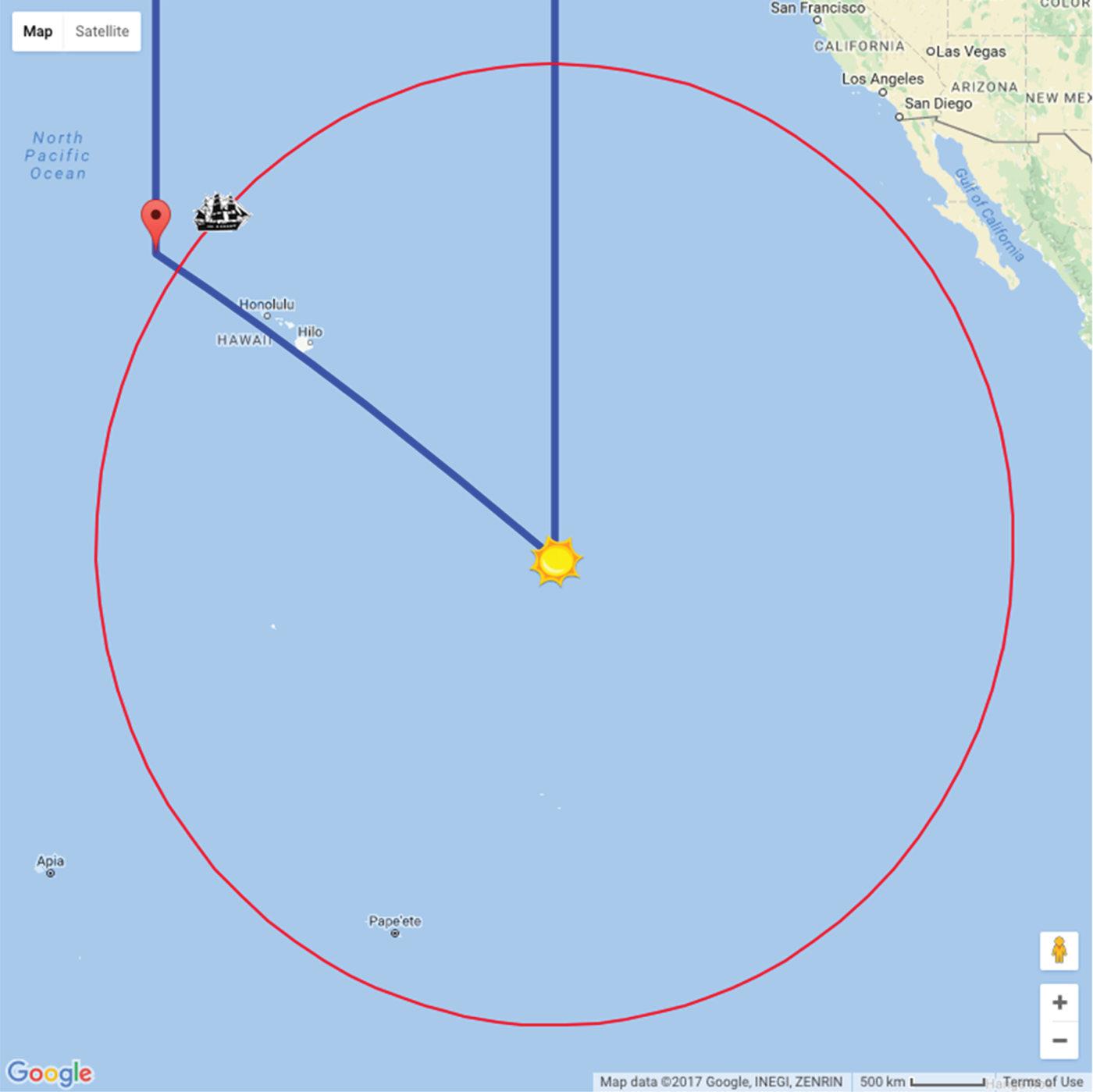
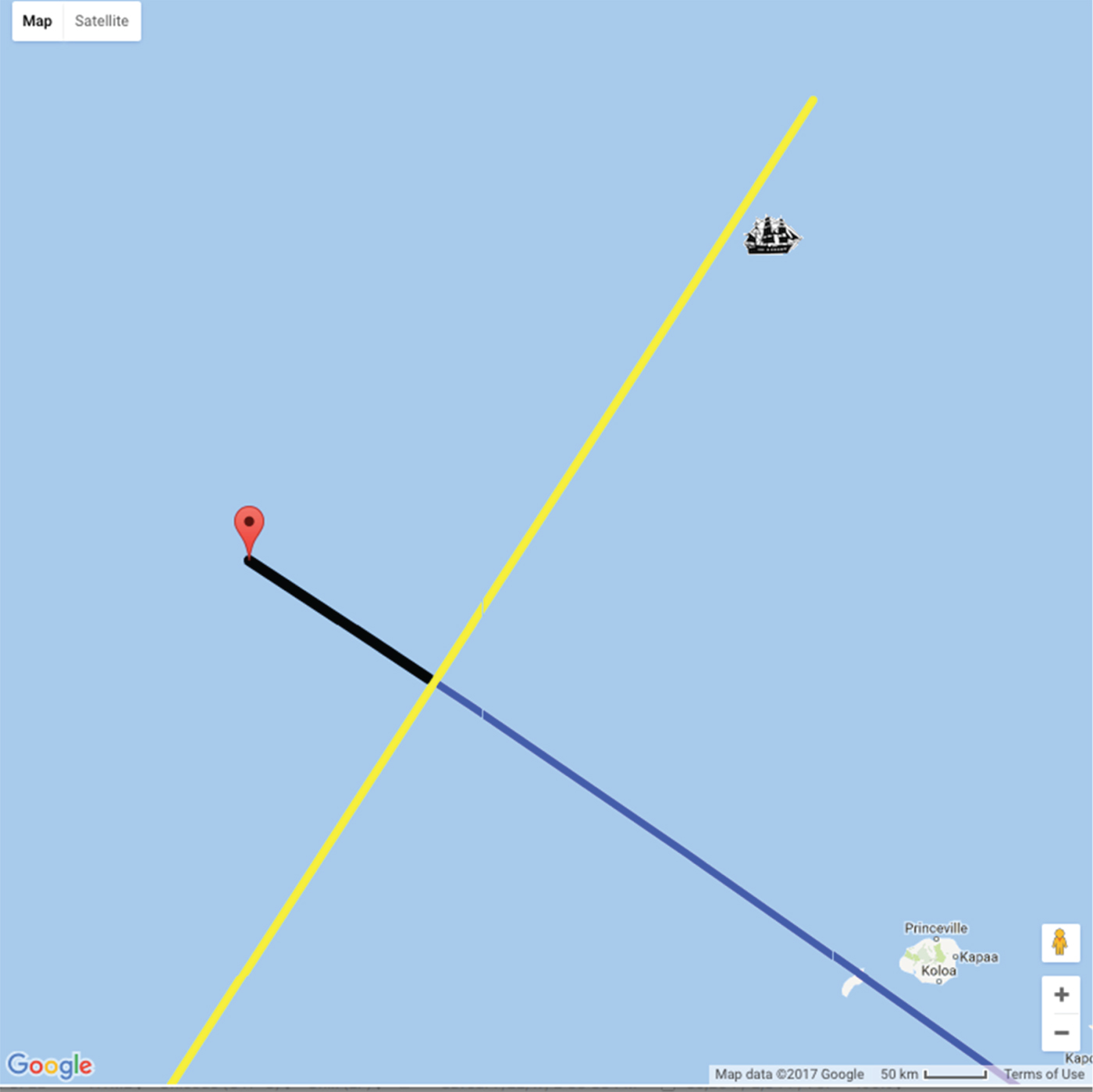
Our work to this point leads to Figure 4, where the red-balloon is placed at the AP, and the navigational triangle is drawn (in blue), using the following code (which is a continuation of code presented above, in particular with the defined variables)
new google.maps.Marker({
map: map,
position: {lat: ap_lat, lng: ap_lng},
});
tri = new google.maps.Polyline({
path: [{lng:gha, lat:90},{lng: gha,lat: decl},
{lng: ap_lng,lat: ap_lat},{lng: ap_lng,lat:90}],
geodesic: true,
strokeColor: ’#0000FF’,
strokeOpacity: 1.0,
strokeWeight: 5
});
tri.setMap(map);
The AP indicated by the balloon, the ship, the Sun's GP, and two sides of the navigational triangle, both ending at the north pole.

We note again the distortion of the triangle due to the map projection, in particular the two sides leading to the North Pole are parallel.
Here side C of Figure 3, or the AP-to-GP connector (hereafter the co-H c , since its measure is 90°-H c ) (Karl, Reference Karl2011) is found by solving for C in
 $$\cos(C) = \cos(A)\cos(B) +\sin(A)\sin(B)\cos(c),$$
giving C = 30·9°. Using this result, Angle b of Figure 3, or the azimuth (Karl, Reference Karl2011) angle, is computed to be b = 123·1° by solving for b in
 $$\cos(B) = \cos(A)\cos(C) +\sin(A)\sin(C)\cos(b),$$
with A the co-latitude of the AP (65·0°), B the co-latitude of the GP (83·8°) and angle c the difference between the Sun's Greenwich Hour Angle (GHA) and the longitude of the AP giving c = 25·7°. A helpful calculator/tutorial can be found in Navy (2017).
Earlier, we stated a hypothetical altitude measurement of the Sun from the ship to be H o = 60·63°. The computed altitude, from the position of the AP is H c = 90·0° − C = 90·0° − 30·9°s or H c = 59·1°. Thus, since H o > H c , the ship must be closer to the GP than the AP (readily observed in Figure 4) by the intercept distance of ΔH = H 0 − H c = 1·53°. Our next computational need is to draw the intercept distance, then draw a line of position (LOP) 1·53° closer to the GP, along and oriented perpendicular to co-H c .
Computing coordinates of an LOP for the sake of plotting is not trivial. Here, we present a method of computing actual (latitude, longitude) coordinates that define the end-points of the LOP, which can lead to other useful calculations, and we note that knowledge of actual LOP coordinates are not normally found in discussions on celestial navigation by the St. Hilaire technique.
To begin, the idea of drawing a line of position indicates the scale of our work is now on a “flat-Earth” section of the ocean, and spherical trigonometry is no longer needed. In this case, the map scale now in use means that moving around in latitude, longitude space is linear in both coordinates, and thus may be thought of as Euclidean (x, y) coordinates. In teaching, this allows us to again emphasise the technique of reducing mechanical mapping errors by concentrating only on a swath (i.e. small, flat-Earth section) of ocean we are interested in, and dispensing with a map that shows both the AP and the GP.
We compute our LOP end-points with the capability of starting at a particular (latitude, longitude) point, and computing a new (latitude, longitude) point after moving at some bearing, along some distance. We use results which are (NIMA, 2015; Stackoverflow, 2015)
 $$\sin(lat) = \sin(AP_{lat})\cos(60{\cdot} \Delta H/R) + \cos(AP_{lat})\sin(60 {\cdot} \Delta H/R)\cos(\theta),$$
and
 $$\tan(long- AP_{ing}) =\displaystyle{{\sin(\theta)\sin(60{\cdot}\Delta H/R)\cos(AP_{lat})}\over{\cos(60{\cdot} \Delta H/R) - \sin(AP_{lat})\sin(lat)}}.$$
Here (lat, long) are the latitude and longitude of the final position, (AP lat , AP lng ) are the latitude and longitude of the AP (or the starting point), ΔH is the distance to move (the intercept distance), R is the radius of the Earth (3,443·92 NM for Google Maps), and θ is the bearing with north being 0°. The factor of 60 scales the ΔH into NM.
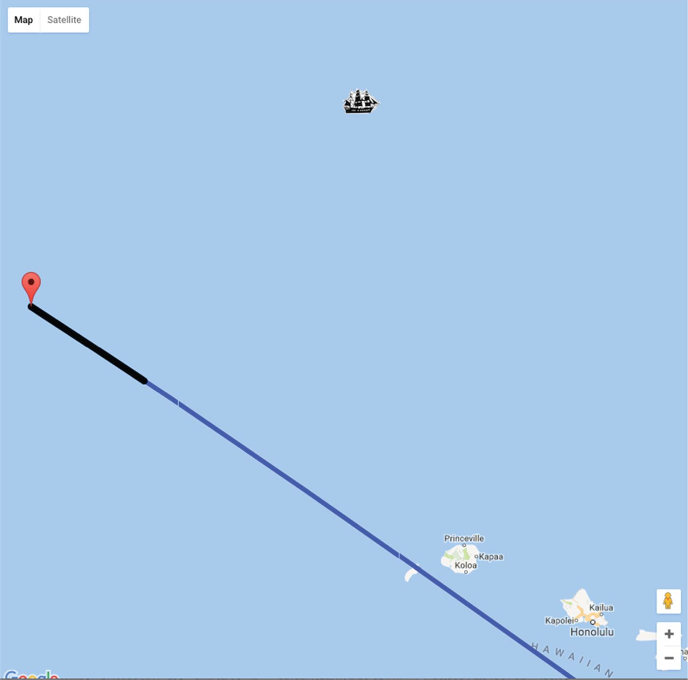
We use this result in two ways. The first is to plot the intercept distance, which involves starting at the AP and moving a distance ΔH either toward or away from the GP (in this case, toward). The bearing is angle b from Figure 3, which was found above to be b = 123·1°, and is thus θ. Using this, we find the coordinates of the intercept line end-point (opposite to the AP) to be (24·1N, 163·6W), and are able to plot this with the thick black line shown in Figure 5. This coordinate is also the point through which the LOP will pass.
The intercept line drawn as the thick black line leading toward the GP, relative to the AP.

The second use of Equations (3) and (4) is to find the two end-points of the LOP. In order to do so, we start at the intercept point above, and move an arbitrary distance (the length of the LOP) at a bearing angle of b + 90° and b − 90°. In this case, the two LOP end-points are found using Equations (3) and (4) to be (17·1N, 168·3W) and (31·0N, 158·3W). The LOP is shown in Figure 6, as drawn using another Polyline construct as used in drawing the navigational triangle above.
The computed LOP now rendered.

In Figure 6, the LOP does not pass directly through the ship, and we immediately cite a few instructional reasons for this. The first being that the LOP is only an approximation for the actual COP on which the ship is located (but lines are geometrically and mathematically easier to deal with than circles). Second, in this work, we avoid taking sights of objects at very high altitudes, to avoid small COPs whose high curvature would be hard to represent with a line.
Having actual (x, y) points for the LOP affords two unique opportunities. The first is to return to a paper-map exercise with students, perhaps giving them actual (x, y) coordinates to plot, and allowing them to verify the LOP is perpendicular to co-H c , etc. The second allows us to check our results in two ways. In the first, the shortest distance between the LOP and the ship's actual position can be computed using a method from high school geometry, that allows us to compute the intersection point between the LOP and a line perpendicular to it, that also passes through the ship's position (Stackoverflow, 2015). In this case, we get about 15 NM, which compares nicely with that obtained by using the scale indicator in the map's legend. This number thus can serve as an error indicator on how our efforts to locate the lost ship are proceeding. The second way is that clicking on the map (as on the LOP, etc.) returns the latitude and longitude of the click in the browser console, allowing for manual numerical inspection of visuals produced in the map.
We have thus concluded a numerically precise, Google Maps-based sight-reduction, that we feel is much more gratifying relative to our previous lessons that used chalkboard sketches, freehand computer drawing programs, or compass and ruler work on paper. However, we still have not determined the location of the lost ship.
3.3. Additional sight-reductions
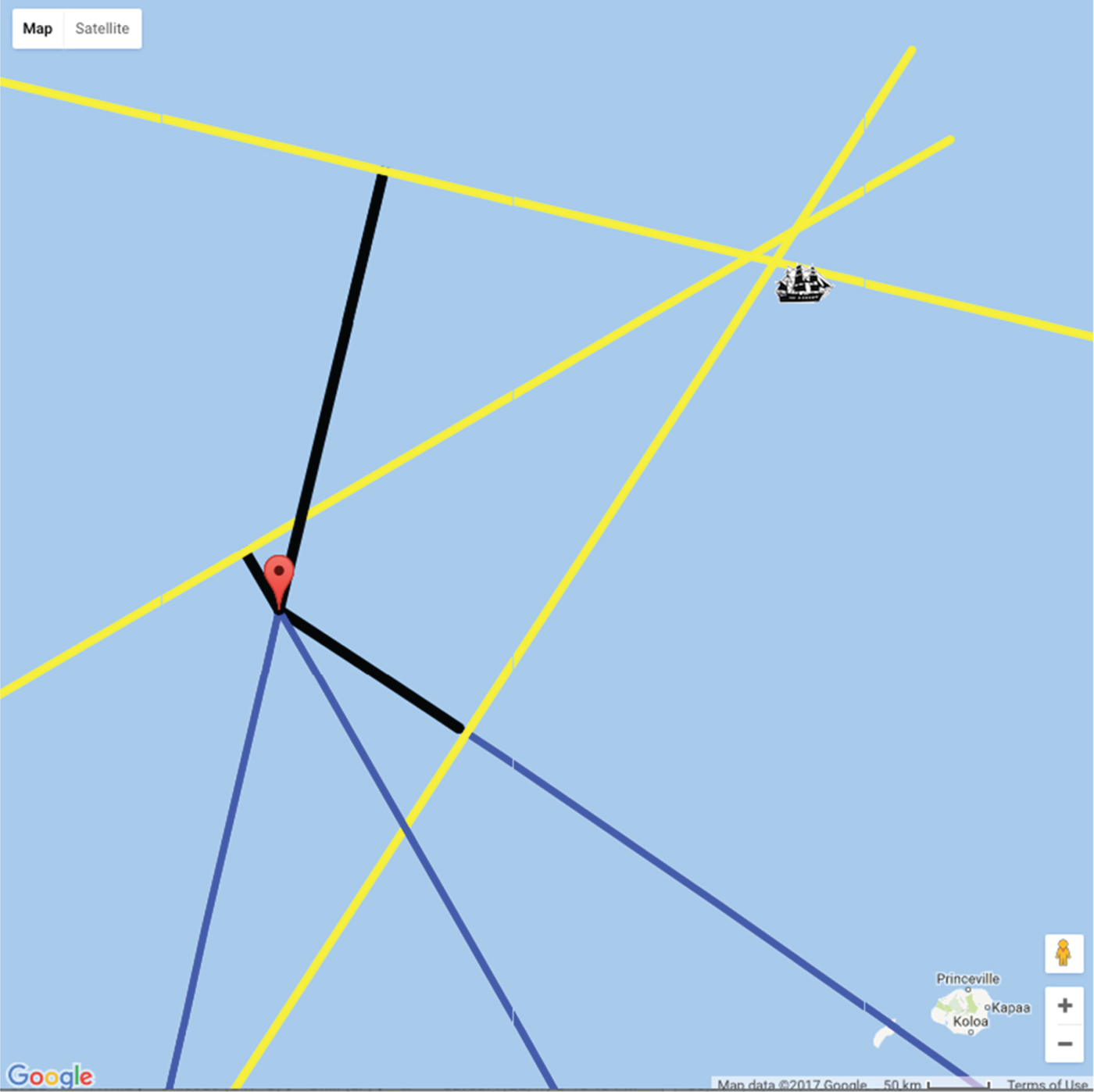
In our lessons, we repeat the above procedure twice more, at one-hour intervals, which resets the ship/AP/GP configuration, as the Sun's GP moves further westward per hour. Ultimately, we arrive at the three-line fix shown in in Figure 7, in which the following “(declinations, GHA) at altitude” triples for the Sun were used: (6·2°N, 139·3°) at 60·6°N, (6·2°N, 154·3°) at 68·0°, and (6·2°N, 169·3°) at 67·4°.
Three lines of position, as a result of a three time delayed shots of the Sun.

With the map automation used here, repeating the procedure is only a matter of updating the GP coordinates of the Sun, and re-running the code. A total of three Sun-sights here result in a small “cocked hat”: (Anderson, Reference Anderson1952; NIMA, 2015; Denny, Reference Denny2012).
As always in the case of celestial navigation, the meaning and conclusions of this result are open to discussion and interpretation, including how to proceed. Here, the three (x, y) points at which the three LOPs intersect, were averaged to find a point “centred” within the cocked hat. This is our first estimate, in terms of actual coordinates, of the position of the ship, which is (27·4N, 161·0W). These agree with the coordinates of (27·8N, 161·0W) found using a manual plotting technique, graciously performed by one of the reviewers of this work. The distance between this point and the ship again allows us to quantify our progress in narrowing our ship's location. In this case, the cocked-hat centre is 18 NM from the ship. Thus, we have improved upon our initial “best guess position” (the AP), by 93%, which was initially 265 NM from the ship. We do not claim these results to be a rigorous proof of celestial navigation, as (for the sake of our lessons), we have stuck with “best practices” of for example, not working near the poles and using altitudes between 10° and 70°, etc.
4. NUMERICAL EXPERIMENTS
With the automated sight-reduction code in hand, we are now free to investigate some nuances of the technique. Below we will denote Δr AP as the distance between the initial AP and the ship, and Δr CH as the distance between the eventual cocked-hat and the ship. Our interest here is in the eventual outcome of Δr CH relative to the initial Δr AP .
4.1. Dependence of final cocked-hat to ship proximity as a function of the initial AP
As mentioned earlier, justifying the meaning and use of the AP is a goal of ours, and now we can demonstrate the role and ramifications of the AP, by systematically testing how Δr AP affects Δr CH , or in other words how does the choice of the AP affect the position of the resulting three-LOP cocked-hat?
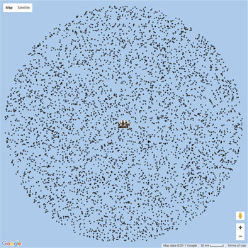
Here we seed the code with 5,000 random APs, that are within a circular area around the ship, with a radius of approximately 150 NM, as shown by the black dots in Figure 8.
5,000 random APs to seed an automated sight-reduction simulation.

From these random initial AP points, Δr AP versus the resulting Δr CH are recorded. In Figure 9, the amount (or factor) the AP was corrected by, or Δr AP /Δr CH versus the ingoing Δr AP is plotted, illustrating several ramifications of the choice of the AP.
The resulting correction factor to the initial AP-to-ship distance, as a function of the initial AP-to-ship distance.

Noting that
 $\Delta r_{AP}/\Delta r_{CH} > 1$
means the ingoing Δr
AP
results in a Δr
CH
that is closer to the ship; we can now finally show students that at some level, the initial selection of the AP does not really matter (even if it was derived from the vilified DR position). The baseline seen in Figure 9 has a slope of approximately 0·1 NM−1, meaning that using this approach, one can always expect one's corrected position to be closer to the ship by at least 10% of the magnitude of the initial Δr
AP
. Larger values of Δr
AP
(i.e. sloppier initial APs) can experience even larger corrections.
Bowditch's curious recommendation (NIMA, 2015) of choosing APs within 40 NM (or so) of the ship is illustrated here as well. With any AP in this range, the correction factors (Δr
AP
/Δr
CH
) in Figure 9 all fall on a line, meaning any Δr
AP
will be reduced by a fixed proportion of its own magnitude. Thus Δr
AP
and the resulting Δr
CH
are related by a multiplicative constant, as in
 $\Delta r_{CH}=k \Delta r_{AP}$
, with k = 0·1 NM−1 here. After the n-th iteration,
 $\Delta r^{\lpar n\rpar }_{CH}= k^{n}\Delta r^{\lpar 0\rpar }_{AP}$
. This recurrence relation results in a geometric progression for the eventual
 $\Delta r^{\lpar n\rpar }_{CH}$
, as seeded by the initial
 $\Delta r^{\lpar 0\rpar }_{AP}$
With k < 1, values of Δr
CH
will exponentially approach a minimum value. Thus, Bowditch must have been referring to navigators experiencing large and gratifying positional corrections for initial APs within this range.
5. USING THE COCKED-HAT POSITION AS THE INITIAL AP FOR A NEW SIGHT-REDUCTION
As alluded to above, it is natural for students to suggest that we next proceed here by using a cocked-hat position as a new “assumed position”, to seed another sight-reduction process. We investigate the ramifications of doing so in this section.
We prepare our code to work with nine sights of the Sun, beginning at 18:20 GMT on 5 April 2015, taking sights in hourly increments until 02:20 GMT on 6 April 2016. We then take more hourly sights starting at 18:00 GMT on 2015-April 6. After determining a three-sight fix, the centre of the resultant cocked-hat is used as the AP for another three-sight fix in the following manner. Fix 1 is found using the Sun's GP at times 18:20, 19:20, and 20:20 GMT. Fix 2 is found from the Sun's GP at times 19:20, 20:20, and 21:20 GMT, and so on, with the AP for the fix after iteration n being the cocked-hat result from fix n − 1.
The resultant cocked-hat positions are shown in Figure 10, along with a graph of Δr CH vs n (inset). In this plot, “AP” is the initial assumed position, “S” is the location of the ship, and the black dots are the sequence of cocked-hat positions produced. Both the plot and its inset show how the initial AP (23·63N, 155·2W) produces values for Δr CH that rapidly approach the ship with each iteration. Eventually the cocked-hat positions converge to a location about 10 NM from the ship.
Evolution of the AP (black dots) relative to the original AP (at “AP”) and the ship (as “S”). Inset: Distance of the cocked hat to the ship as a function of iteration number.

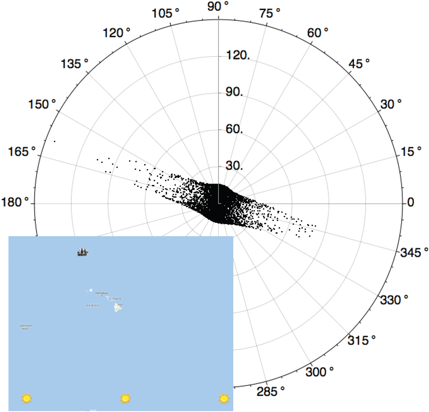
Lastly, we wonder from Figure 8, if there are any preferred angular positions for the initial AP, that lead to larger distance reduction factors Δr AP /Δr CH , than others. Figure 11 is a scaled version of Figure 8, showing a polar plot of Δr AP /Δr CH versus the initial angle of a given AP used in Figure 8. (Here we use standard polar axes from mathematics in both Figure 8 and 11, with 0° toward the right with positive angles counter-clockwise.) In Figure 11, the elongated direction of the points is oriented in the general direction of the three GPs used in determining the final cocked-hat positions (see inset Figure 11). Thus, there is a strong bias to obtain larger values of Δr AP /Δr CH for APs chosen along an azimuth on or near that of the one connecting the ship and GP. This is perhaps simple to explain, but insightful nonetheless: if an AP is chosen on the same azimuth as that connecting the ship and the GP, then the ΔH correction will place the LOP directly on the ship, resulting in a full correction to one's position. Those in directions orthogonal to the ship-GP azimuth are limited in how close the ΔH correction can “slide” an LOP onto the location of the ship.
Polar plot of the points shown in Figure 8, displaying a strong bias toward initial APs that lie approximately on the ship-GP azimuth to yield large corrections to one's position. Inset: Position of the lost ship relative to the GPs used in the sight-reduction process.

6. CONCLUSIONS
Born out of our frustration with teaching aids available for classical celestial navigation, we have developed and presented a numerically precise, highly adaptable, and visual demonstration of a sight-reduction plan, using a programming approach to Google Maps. We used it to demonstrate the technique of St. Hilaire, and to analyse the effects and meaning of the assumed position. Future work involves developing our code into a fully interactive web-based tutorial on celestial navigation. We also wish to complement the web-based tutorials with a simple planar model, so “rules of thumb” on celestial navigation can be more readily relayed to students. These efforts are underway, and will likely be presented in a future paper.
ACKNOWLEDGMENTS
The author is indebted to Professor R. Holtzapple for his proofreading of this manuscript and helpful suggestions and P. Stegner for his encouragement during long “research afternoons” in the British Library during the summers of 2014 and 2017. We also thank the Cal Poly International Center for the opportunity to teach and study in London, and London-based Foundation for International Education (FIE) for their hospitality. Also, we are deeply indebted to an anonymous reviewer who took the time to run and recreate some of our Javascript/Google Map ideas, and another who ran our numbers through a manual plotting exercise, both helping us find numerical errors in our original code. Thank you both for your diligence.