


Introduction
Kelp, large brown macroalgae primarily of the Order Laminariales, are distributed on temperate and sub-polar reefs along ∼36% of global coastlines (Jayathilake and Costello, Reference Jayathilake and Costello2021). Here, they form extensive, highly productive and diverse forests that provide a range of valuable ecosystem goods and services (Beaumont et al., Reference Beaumont, Austen, Mangi and Townsend2008; Smale et al., Reference Smale, Burrows, Moore, O’connor and Hawkins2013; Eger et al., Reference Eger, Marzinelli, Beas-luna, Blain, Blamey, Byrnes, Carnell, Choi, Hessing-lewis, Kim, Kumagai, Lorda, Moore, Nakamura, Pérez-matus, Pontier, Smale, Steinberg and Vergés2023). As foundation species, kelp create biogenic habitat and support diverse associated assemblages and food webs through high primary productivity (Mann, Reference Mann1973; Dayton, Reference Dayton1985; Teagle et al., Reference Teagle, Hawkins, Moore and Smale2017; Rassweiler et al., Reference Rassweiler, Reed, Harrer and Nelson2018), alongside playing an important role in coastal processes such as wave attenuation (Pinsky et al., Reference Pinsky, Guannel and Arkema2013), nearshore sedimentation (Connell, Reference Connell2005), nutrient cycling (Pfister et al., Reference Pfister, Altabet and Weigel2019), and carbon storage (Pessarrodona et al., Reference Pessarrodona, Moore, Sayer and Smale2018).
Although kelp forests can play an important role in ecological and biogeochemical processes, the degree to which they do so is generally governed by their structure and spatial extent (Morris et al., Reference Morris, Graham, Kelvin, Ghisalberti and Swearer2020). The structure and distribution of kelp forests is controlled by an array of interacting physical processes including temperature (Wernberg et al., Reference Wernberg, Bennett, Babcock, Bettignies, Cure, Depczynski, Dufois, Fromont, Fulton, Hovey, Harvey, Holmes, Kendrick, Radford, Santana-garcon, Saunders, Smale, Thomsen, Tuckett and Tuya2015; Smith et al., Reference Smith, Moore, King and Smale2022), light availability (Desmond et al., Reference Desmond, Pritchard and Hepburn2015; Smith et al., Reference Smith, Moore, King and Smale2022), and wave exposure (Harrold et al., Reference Harrold, Watanabe and Lisin1988; Norderhaug et al., Reference Norderhaug, Christie, Andersen and Bekkby2012; Bekkby et al., Reference Bekkby, Rinde, Gundersen, Norderhaug, Gitmark and Christie2014), as well as ecological processes such as competition (Arkema et al., Reference Arkema, Reed and Schroeter2009) and herbivory (Watanabe and Harrold, Reference Watanabe and Harrold1991). These processes vary across geographical regions and depth gradients, resulting in variation in kelp forest structure across multiple spatial scales (Smale et al., Reference Smale, Burrows, Evans, King, Sayer, Yunnie and Moore2016; Smith et al., Reference Smith, Moore, King and Smale2022), and highlighting the importance of depth as a structuring factor. However, in many regions, the structure and functioning of kelp forests is impacted by rapidly changing environmental conditions and increasing pressure from anthropogenic influences (Ling et al., Reference Ling, Johnson, Frusher and Ridgway2009; Arnold et al., Reference Arnold, Teagle, Brown and Smale2016; Provost et al., Reference Provost, Kelaher, Dworjanyn, Russell, Connell, Ghedini, Gillanders, Figueira and Coleman2017; Wernberg et al., Reference Wernberg, Thomsen, Baum, Bishop, Bruno, Coleman, Filbee-dexter, Gagnon, He, Murdiyarso, Rogers, Silliman, Smale, Starko and Vanderklift2024). Climate change is an underlying cause for major changes in kelp forest structure through warming-driven shifts in species’ distributions (Smale et al., Reference Smale, Pessarrodona, King, Burrows, Yunnie, Vance and Moore2020), and marine heatwaves, which are driving the alteration and collapse of kelp forest habitats across multiple continents (Tyler-walters, Reference Tyler-walters2007; Arafeh-dalmau et al., Reference Arafeh-dalmau, Montaño-moctezuma, Martinez, Beas-luna, Schoeman and Torres-moye2019; Smale et al., Reference Smale, Wernberg, Oliver, Thomsen, Harvey, Straub, Burrows, Alexander, Benthuysen, Donat, Feng, Hobday, Holbrook, Perkins-kirkpatrick, Scannell, Sen Gupta, Payne and Moore2019; Filbee-dexter et al., Reference Filbee-dexter, Wernberg, Grace, Thormar, Fredriksen, Narvaez, Feehan and Norderhaug2020). Processes operating across the land-sea interface, such as coastal development and agricultural practices leading to decreased coastal water quality, have also contributed to the degradation and disappearance of kelp forests in many regions (Krumhansl et al., Reference Krumhansl, Okamoto, Rassweiler, Novak, Bolton, Cavanaugh, Connell, Johnson, Konar, Ling, Micheli, Norderhaug, Pérez-matus, Sousa-pinto, Reed, Salomon, Shears, Wernberg, Anderson and Byrnes2016). The impacts of these anthropogenic stressors are likely to intensify in many regions. It is therefore imperative to have a robust understanding of the structure of these key coastal ecosystems to better manage and protect them, and to have a baseline to monitor and restore the system to, should they be negatively impacted in the future.
Kelp forest structure is a key determinant of the quantity of carbon stored within the respective forest. ‘Carbon standing stock’ (CSS), a measure of the quantity of carbon stored within kelp tissues at a specific point in time (Hill et al., Reference Hill, Bellgrove, Macreadie, Petrou, Beardall, Steven and Ralph2015), is primarily determined by the morphology and density of individuals of a specific kelp species, with larger individuals and higher density forests typically storing greater quantities of carbon (Smale and Moore, Reference Smale and Moore2017). Given the potential spatial extent of kelp both globally (∼36% of coastlines; Jayathilake and Costello, Reference Jayathilake and Costello2021) and within the current study area of the United Kingdom (UK; 15,984 km2; Yesson et al., Reference Yesson, Bush, Davies, Maggs and Brodie2015), there is likely to be a significant amount of carbon stored within the habitats they underpin, with estimates suggesting CSS to be 1–2 orders of magnitude greater than other vegetated temperate marine habitats such as seagrass beds or saltmarshes (Garrard and Beaumont, Reference Garrard and Beaumont2014). Kelp also act as ‘carbon donors’, with the vast majority of primary productivity often exported from the source habitat (Krumhansl and Scheibling, Reference Krumhansl and Scheibling2012; Smale et al., Reference Smale, Pessarrodona, King and Moore2022b) and transported to carbon storage habitats where it contributes to the allochthonous organic matter that they sequester (Trevathan-tackett et al., Reference Trevathan-tackett, Kelleway, Macreadie, Beardall, Ralph and Bellgrove2015; Queirós et al., Reference Queirós, Tait, Clark, Bedington, Pascoe, Torres, Somerfield and Smale2023; Filbee-dexter et al., Reference Filbee-dexter, Pessarrodona, Pedersen, Wernberg, Duarte, Assis, Bekkby, Burrows, Carlson, Gattuso, Gundersen, Hancke, Krumhansl, Kuwae, Middelburg, Moore, Queirós, Smale, Sousa-pinto and Krause-jensen2024).
Along the rocky, wave-exposed coastline of the UK, kelp forests are generally dominated by the stipitate kelp Laminaria hyperborea (Gunnerus) Foslie 1884, whose range extends from northern Portugal to northern Norway (Sjøtun et al., Reference Sjøtun, Fredriksen, Lein, Rueness and Sivertsen1993; Pinho et al., Reference Pinho, Bertocci, Arenas, Franco, Jacinto, Castro, Vieira, Sousa-pinto, Wernberg and Tuya2016), reaching depths of >40 m in clear waters (Hiscock, Reference Hiscock1992; Tyler-walters, Reference Tyler-walters2007). Environmental conditions such as light availability and local hydrodynamic regimes vary across shallow subtidal depth gradients, influencing lower depth limits and resulting in L. hyperborea forests being more commonly found from the low intertidal/shallow subtidal to depths of 15–20 m along much of the UK coastline (Smith et al., Reference Smith, Moore, King and Smale2022). In favourable conditions, L. hyperborea forms extensive, dense forests that create habitat both directly (Teagle et al., Reference Teagle, Moore, Jenkins and Smale2018; Earp et al., Reference Earp, Smale, King, Bestwick, Fazel and Moore2024) and indirectly (Sjøtun et al., Reference Sjøtun, Christie and Fosså2006; Bué et al., Reference Bué, Smale, Natanni, Marshall and Moore2020) that in turn support inshore fisheries and coastal biodiversity (Johnson and Hart, Reference Johnson and Hart2001; Norderhaug et al., Reference Norderhaug, Fredriksen and Nygaard2003; Burrows, Reference Burrows2012; Smale et al., 2022). Around a decade ago, our understanding of the ecology of kelp forests along the extensive and complex coastline of the UK lagged behind other leading scientific nations (Smale et al., Reference Smale, Burrows, Moore, O’connor and Hawkins2013), but recent research efforts have characterised the structure and functioning of UK L. hyperborea forests and their associated assemblages, with a particular focus on the northern and western coasts of the UK (Smale et al., Reference Smale, Burrows, Evans, King, Sayer, Yunnie and Moore2016; Smale and Moore, Reference Smale and Moore2017; Teagle et al., Reference Teagle, Moore, Jenkins and Smale2018; Smith et al., Reference Smith, Moore, King and Smale2022; Earp et al., Reference Earp, Smale, King, Bestwick, Fazel and Moore2024; Gouraguine et al., Reference Gouraguine, Smale, Edwards, King, Jackson-bué, Kelly, Earp and Moore2024). Whilst these previous studies show a large degree of variability in L. hyperborea forest structure and functioning across the latitudinal range of the UK, they also show these regions to have some of the most dense and productive kelp habitats within this species range, with individuals reaching over 250 cm in length and forests attaining standing biomass values of >30 kg m−2 (fresh weight [FW]).
Although these previous studies have substantially enhanced our understanding of the structure, functioning and ecosystem services provided by UK kelp forests, they have often overlooked kelp forests along the eastern coast of the UK, despite historical investigations along the North Sea coastline of the UK indicating the presence of extensive L. hyperborea forests (Whittock, Reference Whittock1969). The North Sea coastline of the UK differs in geomorphology from the western Atlantic coastline of the UK, being characterised by broader shallow shelf environments and more gently sloping seabed topography compared to the topographically complex rocky Atlantic coastline (Balson et al., Reference Balson, Butcher, Holmes, Johnson, Lewis, Musson, Henni, Jones, Leppage, Rayner and Tuggey2001; May and Hansom, Reference May and Hansom2003; Masselink et al., Reference Masselink, Russell, Rennie, Brooks and Spencer2018). These differences in coastal geomorphology may influence the spatial extent, structure, and depth distribution of kelp forest habitats, and may contribute to different ecological and structural patterns compared to kelp forests along the Atlantic coastline of the UK. Here, we address this knowledge gap by investigating the structure of L. hyperborea forests along a gradient of depth (2–10 m below chart datum [BCD]) at six survey sites within two regions on the eastern coast of the UK bordering the North Sea. We also examine estimates of CSS for L. hyperborea forests at a further four regions, representing a latitudinal gradient of 9° across the UK and encompassing a range of environmental conditions. This study provides comprehensive insight into the structure of L. hyperborea forests on the North Sea coastline of the UK and allows for additional comparison to be made across much of this species range.
Materials and methods
Kelp forest structure and depth distribution
In June 2021, kelp forests dominated by L. hyperborea were surveyed in two regions along the North Sea coastline of eastern UK: northeast (NE) England (A) and southeast (SE) Scotland (B) (Figure 1). Within each region, three sites were selected based on the following criteria: (1) sites included sufficient areas of rocky subtidal reef at depths of 5 m BCD (all depths hereafter relate to BCD), with two of the three chosen sites in each region characterised by a sloping gradient from 2 to 10 m depth (or the deepest extent of kelp forest); (2) sites were representative of the wider region in terms of coastal geomorphology and not obviously influenced by localised anthropogenic activities (e.g. sewage outfalls); and (3) sites were ‘open coast’ and moderately to fully exposed to wave action. Regions were separated by a distance of 45 km, while sites within regions were separated by 0.3–3.5 km.
Study regions across the United Kingdom: (A) NE England, (B) SE Scotland, (C) N Scotland, (D) W Scotland, (E) SW Wales, and (F) SW England. Small maps indicate locations of study sites within each region. Regions A and B are new survey regions sampled in the present study. Data for the previously sampled regions of C–F are from Smith et al. (Reference Smith, Moore, King and Smale2022).

Figure 1 Long description
The composite image includes six maps showing study regions across the United Kingdom. Each map highlights specific sites within the regions. A) NE England shows sites near Seahouses. B) SE Scotland includes sites near St. Abbs. C) N Scotland features sites around Scourie. D) W Scotland highlights sites near Oban. E) SW Wales shows sites around Milford Haven. F) SW England includes sites near Plymouth. Each map is marked with specific locations and scale bars for reference. The main map of the UK indicates the general location of each study region with labeled boxes corresponding to the detailed maps.
To investigate the structure of L. hyperborea forests, SCUBA divers placed five to eight replicate 1 m2 quadrats haphazardly within the main kelp forest habitat, estimated the per cent cover of the kelp canopy and counted the number of canopy and sub-canopy individuals. Canopy plants were defined as mature sporophytes forming part of the main canopy, while sub-canopy plants included mature sporophytes as well as juveniles with digitate blades and a well-developed stipe found beneath the main canopy. First-year recruits with undivided blades were counted but were excluded from the analyses due to uncertainty in their identification and considerable spatial patchiness. The density of sea urchins (exclusively Echinus esculentus) within quadrats was also recorded. The morphology and biomass of canopy-forming plants were investigated by haphazardly collecting 10 individuals per sampling depth, per site. Whole plants were collected by prising holdfasts from the substratum and returning them to the surface, where morphological characteristics including stipe length (cm), total length (cm), stipe biomass (g FW), and total biomass (g FW) were recorded. Individuals were also aged by counting annual growth rings on cross-sections of the stipe sampled close to the stipe-holdfast junction (as described by Kain and Jones, Reference Kain and Jones1963). Data and sample collection were conducted at 5 m at each of the three chosen sites in each region, with additional sampling taking place at 2 and 10 m (or the deepest extent of kelp forest if shallower than 10 m) at two of the three chosen sites in each region (A2, A3, B2, and B3). At these sites, the maximum depth of the kelp forest was also recorded.
Carbon standing stock
Additional data on the morphology of L. hyperborea in the UK, spanning a further four regions and a latitudinal gradient of almost 9°, were sourced from Smith et al. (Reference Smith, Moore, King and Smale2022). CSS was estimated following the methods of Smale et al. (Reference Smale, Burrows, Evans, King, Sayer, Yunnie and Moore2016), in which the relationship between FW and dry weight (DW) of basal blade, distal blade, and stipe tissue was calculated from 47 kelp plants collected from regions C, D, E, and F (N Scotland, W Scotland, SW Wales, and SW England, respectively; Figure 1). Study-wide averages calculated in Smale et al (Reference Smale, Burrows, Evans, King, Sayer, Yunnie and Moore2016) showed the DW:FW ratio varied between different regions of the kelp plant, with mean values of 0.29, 0.17, and 0.21 for basal blade, distal blade, and stipe, respectively (Smale et al., Reference Smale, Burrows, Evans, King, Sayer, Yunnie and Moore2016). Here, we averaged these values for basal and distal blade DW:FW to obtain a value for the whole kelp blade of 0.23. These values were then used to convert our measurements of whole plant FW from NE England and SE Scotland to whole plant DW. Site averages of DW for canopy-forming L. hyperborea were multiplied by the average density of canopy-forming individuals recorded in the 1 m2 quadrats at each site, giving an estimated biomass (DW) per 1 m2. Finally, the conversion of DW per m2 to CSS was based on previous research on a range of kelp species that indicates approximately 30% of DW is carbon (Smale et al., Reference Smale, Burrows, Evans, King, Sayer, Yunnie and Moore2016; Pessarrodona et al., Reference Pessarrodona, Moore, Sayer and Smale2018).
Environmental data
Data for various environmental variables known to influence kelp forest structure (Smale et al., Reference Smale, Burrows, Evans, King, Sayer, Yunnie and Moore2016) were extracted for comparisons to be made between sites and regions. Wave exposure was determined from log10 wave fetch values extracted from Burrows (Reference Burrows2020), with all study sites categorised as ‘exposed’, with values greater than 3.5 log10 (Burrows, Reference Burrows2012) (Table 1). Sea surface temperature (SST) and chlorophyll a concentration (proxy for turbidity) (Table 1) for the period between 2010 and 2020 were extracted from Bio-ORACLE (Tyberghein et al., Reference Tyberghein, Verbruggen, Pauly, Troupin, Mineur and De Clerck2012; Assis et al., Reference Assis, Fernández Bejarano, Salazar, Schepers, Gouvêa, Fragkopoulou, Leclercq, Vanhoorne, Tyberghein, Serrão, Verbruggen and De Clerck2024). However, due to the proximity of the sites to one another and the resolution of the environmental data (∼5 km2), data were only available on the regional scale and therefore only wave fetch data were used in further analyses.
Environmental drivers of kelp forest structure at six study sites within two regions of NE England and SE Scotland
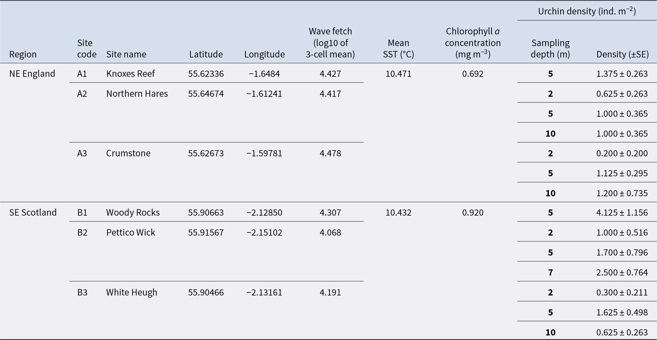
Table 1 Long description
Environmental and site variables are listed for six kelp-forest study sites across NE England and SE Scotland, including coordinates, wave fetch, mean sea surface temperature, chlorophyll a, and urchin density by sampling depth with standard error. Mean sea surface temperature is similar where reported, about 10.4 degrees Celsius at Knoxes Reef and Woody Rocks, while chlorophyll a differs, from 0.692 at Knoxes Reef to 0.920 at Woody Rocks. Wave fetch varies across sites, highest at Crumstone (4.478) and lowest at Pettico Wick (4.068). Urchin density is reported at multiple depths per site and is often highest at 5 m: Knoxes Reef has 5 individuals per square meter at 5 m; Woody Rocks has 4.125 at 5 m; and Pettico Wick rises from 1.0 at 2 m to 2.5 at 7 m. Northern Hares and Crumstone show lower densities overall, with values near 0.2 to 1.2 across 2 to 10 m. White Heugh is low at 2 m (0.3) and higher at 5 m (1.625) before dropping at 10 m (0.625). Comparisons across sites should be made cautiously because urchin density is depth-specific and some environmental variables are not repeated on every depth row.
Mean annual sea surface temperature (SST) and chlorophyll a (proxy for light) values were extracted from Bio-ORACLE and represent averages for the years 2010–2020 (Tyberghein et al., Reference Tyberghein, Verbruggen, Pauly, Troupin, Mineur and De Clerck2012; Assis et al., Reference Assis, Fernández Bejarano, Salazar, Schepers, Gouvêa, Fragkopoulou, Leclercq, Vanhoorne, Tyberghein, Serrão, Verbruggen and De Clerck2024). Wave fetch values were extracted from Burrows (Reference Burrows2020). Urchin density is the average number of Echinus esculentus recorded in 5–8 replicate 1 m2 quadrats at a range of sampling depths at each site.
Statistical analysis
Patterns of spatial variability in L. hyperborea forest structure (i.e. canopy density, total density, and total canopy biomass), individual-level metrics (i.e. canopy former biomass, stipe length, total length, and age), and CSS were analysed using univariate permutational analyses of variance (PERMANOVA) (Anderson, Reference Anderson2001). Variation in kelp forest metrics between all sites in NE England (A) and SE Scotland (B) at 5 m depth was determined using two-way PERMANOVAs with Region (fixed, two levels) and Site (random, three levels and nested within Region) as factors. Variation in kelp forest metrics between two sites in NE England (A) and SE Scotland (B) and across depths was determined using three-way PERMANOVA with Region (fixed, two levels), Site (random, two levels and nested within Region), Depth (fixed, three levels), and their interactions as factors. Variation in CSS between sites at the six study regions (A–F; Figure 1) at 5 m depth was determined using a two-way PERMANOVA with Region (fixed, six levels) and Site (random, two levels and nested within Region) as factors. For each analysis, permutations (9999 under a reduced model) were based on Euclidean distance similarity matrices constructed from untransformed data. Where the number of permutations was low (i.e. <100), p-values derived from Monte Carlo simulations were used. Pairwise post hoc comparisons were performed where significant differences (p < 0.05) were detected.
Relationships between log10 values of wave fetch and kelp forest structure (i.e. canopy density, total density, and total canopy biomass) and individual-level metrics (i.e. canopy former biomass, stipe length, total length, and age) at a depth of 5 m were examined using distance-based linear models (DISTLMs). The relationship between urchin density and the maximum kelp forest depth was also tested using DISTLM. All DISTLMs were based on Euclidean distance similarity matrices and run using 9999 permutations, which is equivalent to carrying out univariate simple linear regression (Anderson et al., Reference Anderson, Gorley and Clarke2008). Statistical analyses were conducted using PRIMER 7 software (Clarke and Gorley, Reference Clarke and Gorley2015) with the PERMANOVA add-on (Anderson, Reference Anderson, Gorley and Clarke2008). Model assumptions, including tests for normality and homogeneity of variance (Q–Q plots, Shapiro–Wilk’s test, and Levene’s test), were checked and confirmed to conform to assumptions of respective analyses, and all figures were made in RStudio v. 4.2.1 (R Core Team, Reference Team2022) using the packages ‘car’ (Fox et al., Reference Fox, Weisberg and Price2001), ‘ggplot2’ (Wickham, Reference Wickham2016), ‘ggpubr’ (Kassambara, Reference Kassambara2016), and ‘rstatix’ (Kassambara, Reference Kassambara2019).
Results
Spatial variability in the structure of L. hyperborea forests
At 5 m depth, L. hyperborea dominated at all sites in NE England and SE Scotland (100% of canopy-forming individuals recorded in quadrats), although the kelp species Alaria esculenta and Saccharina latissima were observed in very low abundances at some sites. The mean (±SE) density of canopy-forming L. hyperborea individuals ranged from 7.3 ± 0.5 to 12.3 ± 0.5 ind. m−2 (B2 and B1, respectively), while the total density of individuals (canopy and subcanopy) ranged from 16.8 ± 2.6 to 32.0 ± 5.1 ind. m−2 (B2 and A2, respectively; Figure 2A and B). Both canopy density and total density varied across small spatial scales, with significant variation between sites nested within regions, but not between regions (Table 2; Figure 2A and B). Stipe length and total length of canopy-forming individuals showed significant small-scale variation between sites nested in regions, with the latter also varying significantly between regions (Table 2). Indeed, the total length of canopy-forming individuals was significantly greater in NE England (272.8 ± 8.5 cm) compared to SE Scotland (196.5 ± 6.6 cm; Figure 2D; Table 2). The stipe length of canopy-forming individuals ranged from 83.6 ± 8.3 to 170.0 ± 2.5 cm (B2 and A1, respectively; Figure 2C).
Structure of Laminaria hyperborea populations at sites within regions A (NE England) and B (SE Scotland) at a depth of 5 m BCD. Bars represent mean values ± SE (n ≥ 6 for quadrat-level variables: A, B, and F; n ≥ 9 for plant-level variables: C, D, E, and G). FW, Fresh weight; Ind., individual. Points show raw data values.
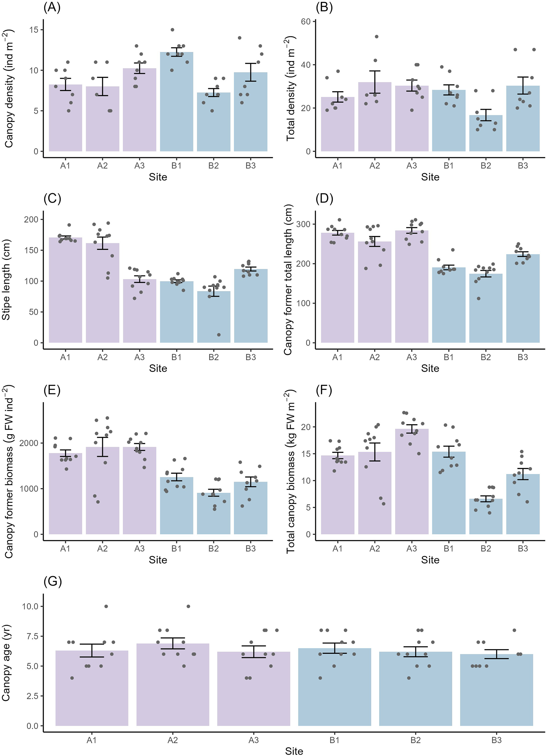
Figure 2 Long description
Multiple bar charts labeled A to G, each comparing different variables across sites A1, A2, A3, B1, B2 and B3. Chart A shows canopy density in individuals per square meter, with site A1 having the highest density and B3 the lowest. Chart B displays total density, where A2 is highest and B3 is lowest. Chart C illustrates stipe length in centimeters, with A1 having the longest and B3 the shortest. Chart D presents canopy-forming total length, with A1 being the longest and B3 the shortest. Chart E shows canopy-former biomass in grams fresh weight per individual, with A1 having the highest biomass and B3 the lowest. Chart F displays total canopy biomass in kilograms fresh weight per square meter, with A1 having the highest and B3 the lowest. Chart G shows canopy age in years, with A1 having the oldest and B3 the youngest. Each chart includes overlaid points representing raw data values and error bars indicating variability. The charts collectively highlight differences between sites in NE England and SE Scotland, with site A1 generally showing higher values across most variables compared to B3.
Univariate permutational ANOVAs to test for variability in population and individual-level kelp metrics between regions and sites at a depth of 5 m BCD
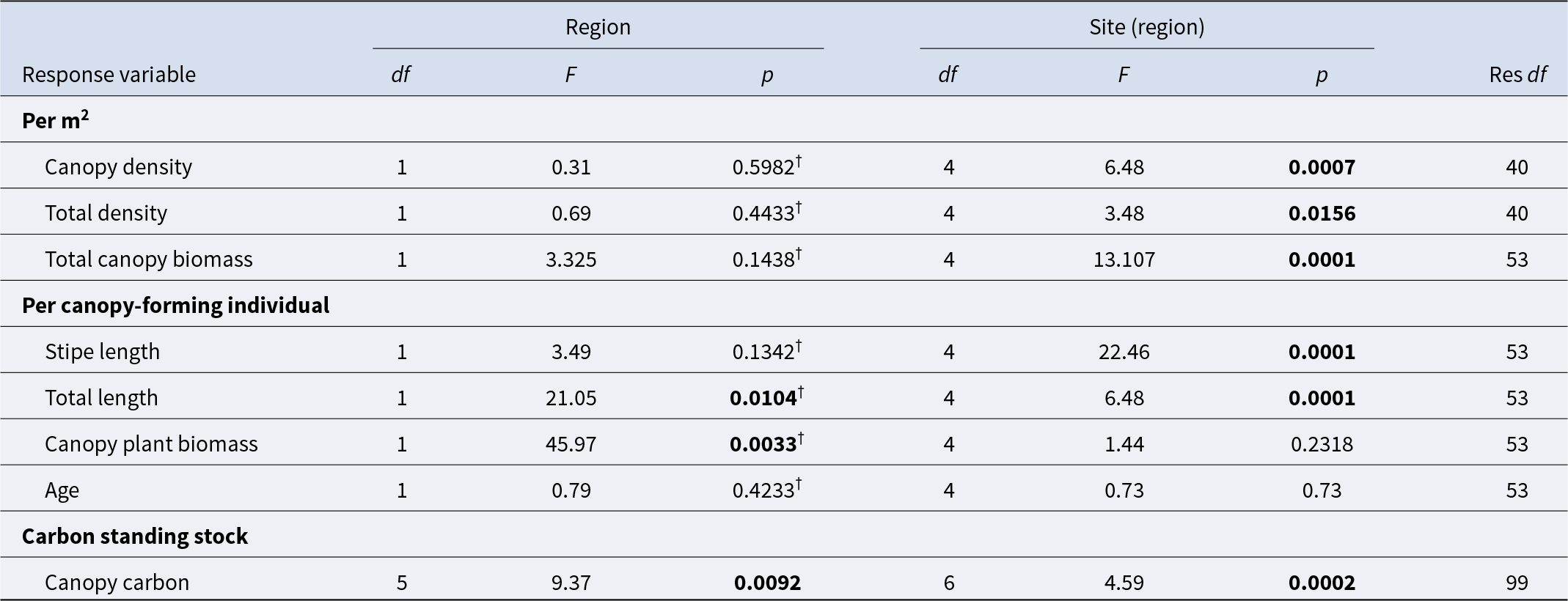
Table 2 Long description
Univariate permutational ANOVA results compare variability in kelp density, biomass, size, age, and canopy carbon at 5 m depth across regions and among sites nested within regions. For per square meter metrics, region is not significant for canopy density, total density, or total canopy biomass, but site within region is significant for all three, with strongest site effect for total canopy biomass. For per canopy-forming individual metrics, region is significant for total length and canopy plant biomass, while stipe length and age show no region effect. Site within region is significant for stipe length and total length, but not for canopy plant biomass or age. Canopy carbon standing stock tested across six regions shows significant differences by region and also by site within region. Several region-level p values are flagged as coming from Monte Carlo simulations, so those specific region inferences should be treated with added caution.
Models were run using 9999 permutations based on similarity matrices derived from Euclidean distances, with ‘Region’ as a fixed factor and ‘Site’ as a random factor nested within ‘Region’. Analysis of carbon standing stock values was carried out between six regions (A–F; Figure 1). All other variables were tested between two regions (A and B; Figure 1). Significant values (p < 0.05) are indicated in bold. Significance values followed by a ‘†’ are derived from Monte Carlo simulations due to the low number of unique permutations.
The biomass of individual canopy formers was significantly greater in NE England (1869.2 ± 118.9 g FW ind−1) compared to SE Scotland (1105.7 ± 88.6 g FW ind−1), whereas the total canopy biomass ranged from 6.6 ± 0.6 to 19.6 ± 0.8 kg FW m−2 (B2 and A3, respectively) and exhibited significant variation between sites nested in regions, but not between regions (Table 2; Figure 2E and F). The age of canopy-forming individuals ranged from 6.0 ± 0.4 to 6.9 ± 0.5 years (B3 and A2, respectively) and did not vary significantly across sites or regions (Table 2; Figure 2G).
Environmental drivers
All study sites were considered ‘exposed’; however, sites in NE England had greater wave fetch values compared to those in SE Scotland (Table 1). Whilst data were only available on the regional scale for other proposed environmental drivers (and not used in analysis), mean SST was comparable between regions, being just 0.04°C greater in NE England than in SE Scotland, and mean chlorophyll a concentration (proxy for light) was roughly 0.2 mg m−3 greater in SE Scotland than in NE England.
When testing the relationship between wave fetch and measures of kelp forest structure, DISTLM tests found significant relationships between wave fetch and total density, as well as all measures of morphology (stipe and total length and canopy former biomass) (Supplementary Table S1), with sites characterised by greater wave exposure supporting greater densities, longer lengths, and overall greater canopy plant biomasses.
Depth distribution of kelp forests in NE England and SE Scotland
At the four sites where kelp forests were studied across a depth gradient, L. hyperborea was dominant at all depth increments. Kelp forest structure was highly variable over small spatial scales, with significant variation in most individual and population-level metrics between sites nested within regions and depths (Table 3; Figure 3).
Univariate permutational ANOVAs to test for variability in population and individual-level kelp metrics between regions, sites, and depths
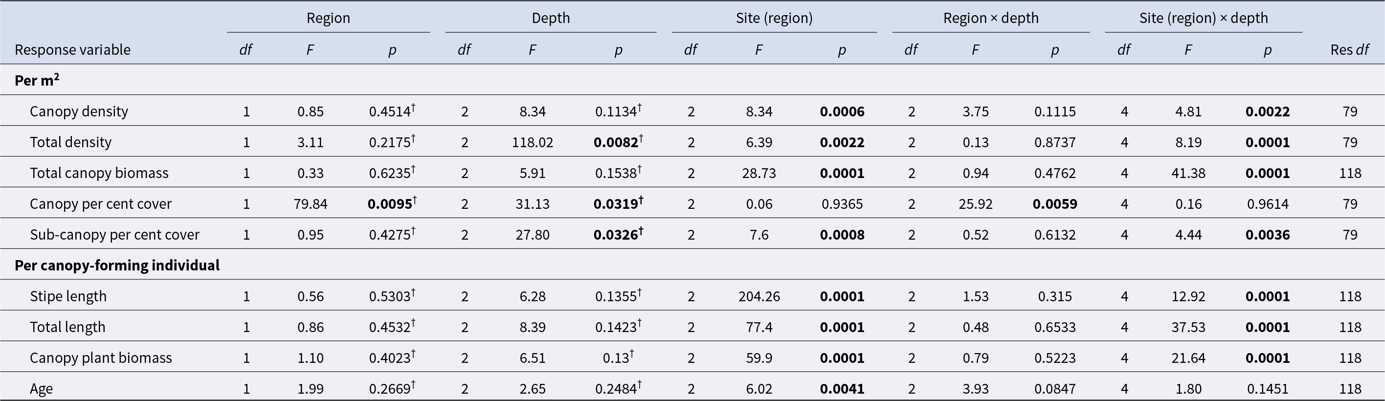
Table 3 Long description
Univariate permutational ANOVA results test how kelp abundance, cover, and individual traits vary by region, depth, site nested within region, and their interactions. For per square meter metrics, depth is significant for total density and canopy percent cover, and site within region is significant for canopy density, total density, total canopy biomass, and sub-canopy percent cover. Region is only significant for canopy percent cover, indicating a clear difference between regions for that response while most others do not differ by region alone. Several responses show strong depth-related variability that depends on site, with site-by-depth significant for canopy density, total density, total canopy biomass, sub-canopy percent cover, and all three individual size or biomass measures. For per individual metrics, site within region is consistently significant for stipe length, total length, canopy plant biomass, and age, while depth alone is not significant for these traits. Region-by-depth is significant only for canopy percent cover, suggesting depth patterns differ between regions for that cover metric but not for the other responses. Some p-values are based on Monte Carlo simulation due to limited unique permutations, so borderline results should be interpreted cautiously.
All variables were tested between two regions (A and B; Figure 1). Models were run using 9999 permutations based on similarity matrices derived from Euclidean distances, with ‘Depth’ and ‘Region’ as fixed factors and ‘Site’ as a random factor nested within ‘Region’. Significant values (p < 0.05) are indicated in bold. Significance values followed by a ‘†’ are derived from Monte Carlo simulations due to the low number of unique permutations.
Structure of Laminaria hyperborea populations at sites within regions A (NE England) and B (SE Scotland) at depths of 2, 5, and 7–10 m BCD. Bars represent mean values ± SE (n ≥ 6 for quadrat-level variables: A, B, and F; n ≥ 9 for plant-level variables: C, D, E, and G). FW, Fresh weight; Ind., individual. Points show raw data values.
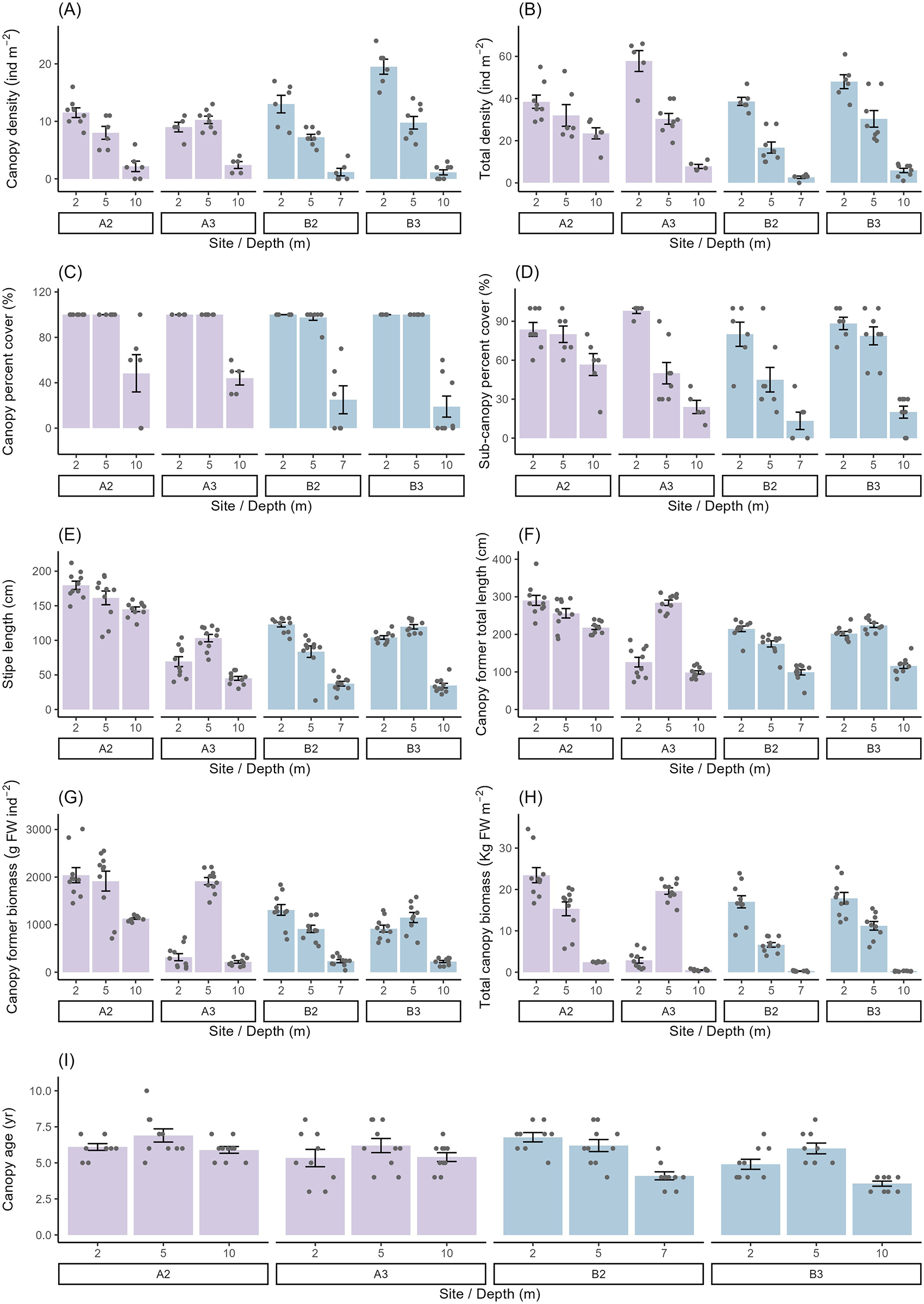
Figure 3 Long description
Nine bar graphs labeled A to I, each representing different kelp forest metrics across sites A2, A3, B2 and B3 at depths of 2 meters, 5 meters and 10 meters. Graph A shows canopy density in individuals per square meter, with site A3 at 5 meters having the highest density. Graph B displays total density in individuals per square meter, with site B3 at 10 meters showing the highest value. Graph C illustrates canopy percent cover, where site A2 at 2 meters has the highest cover. Graph D presents sub-canopy percent cover, with site B2 at 5 meters showing the highest value. Graph E shows stipe length in centimeters, with site A3 at 5 meters having the longest stipe length. Graph F displays total length in centimeters, with site B3 at 10 meters showing the longest total length. Graph G illustrates canopy plant biomass in grams per square meter, with site A3 at 5 meters having the highest biomass. Graph H presents total canopy biomass in kilograms per square meter, with site B3 at 10 meters showing the highest biomass. Graph I shows canopy age, with site A2 at 2 meters having the oldest canopy. Each graph includes mean values with error bars indicating standard error and individual data points are plotted. The x-axis of each graph represents site and depth, while the y-axis represents the respective metric values. The graphs use different colors to distinguish site groups, aiding in visual differentiation. Overall, site B3 at 10 meters tends to have higher values for density and biomass, while site A2 at 2 meters shows higher canopy cover and age, indicating variability in kelp forest structure across sites and depths.
The density of canopy-formers and the total density of L. hyperborea tended to decrease with increasing depth at all sites (Figure 3A and B). However, there was significant variability between sites nested in region and depths (Table 3; Figure 3A and B) driven by non-significant declines in density between 2 and 5 m depth at a limited number of sites, as well as variability in kelp density at 2 m for some sites. In terms of L. hyperborea canopy per cent cover, there was a significant region by depth interaction (Table 3), with cover at 10 m being lower in SE Scotland compared to NE England (Figure 3C). In contrast, at all other depths, canopy cover was similar across sites and regions, with values often reaching 100% (Figure 3C). For sub-canopy plants, there was a significant interaction between sites nested within regions and depths (Table 3). In general, per cent cover of sub-canopy individuals decreased with depth at all sites, although the rate of decline varied between sites (Figure 3D). Total canopy biomass also varied between sites nested within regions and depths (Table 3). At all sites, total canopy biomass was lowest at 10 m, but there was significant variation between sites and regions, while the greatest total canopy biomass occurred at 2 m at all sites except A3, where it occurred at 5 m (Figure 3H).
Stipe length, total length, and canopy plant biomass varied significantly between sites nested in regions and depths (Table 3; Figure 3C, E, and F). As with L. hyperborea density, there was a tendency for all these factors to decrease with depth, with the exception of site A3 and B3, where these metrics increased from 2 to 5 m and then decreased again down to 10 m depth (Figure 3E and G). Stipe length and total length were generally greater at site A2 compared to site A3 across all depth ranges, with the exception of total length at 5 m, which was greater at site A3. The age of canopy-forming L. hyperborea plants did not vary with depth but did vary across sites nested within regions, with A3 (5.7 ± 0.5 years) and B3 (4.8 ± 0.3 years) supporting younger canopy-forming plants compared to A2 (6.3 ± 0.3 years) and B2 (5.7 ± 0.3 years) (Table 3; Figure 3I).
Kelp forest maximum depth was greatest in NE England at site A2, where it reached 13 m, whereas at site A3 it reached only 11 m. Maximum kelp forest depth in SE Scotland was considerably lower than in NE England, reaching just 7 m at site B2 and 10 m at site B3 (Supplementary Table S2). Although there was no significant relationship between the density of urchins and the maximum depth penetration of kelp forests (Supplementary Table S3), the relationship did approach significance (p = 0.07), with the highest urchin density being recorded at the site with the shallowest kelp forest depth penetration (7 m at site B2). No trend in urchin abundance and kelp forest depth was observed across the other three sites.
Carbon standing stock
The study-wide average of CSS from our six sampling regions (A–F; Figure 1) held within L. hyperborea canopies was 858 ± 79 g C m−2 (Table 4). The standing stock of carbon varied significantly between sites nested within regions (Table 2) and was greatest at site C1 (N Scotland; 1578 ± 94 g C m−2) and lowest at site E1 (SW Wales, 303 ± 38 g C m−2) (Figure 4). Variability among sites within a region was most pronounced in SE Scotland (B), where standing stock varied by ∼51% between sites, and was least pronounced in SW England (F), where variation was just ∼11% (Figure 4). While there were clear differences between most sites nested within regions, there were also some clear regional effects (Table 2). With the exception of SE Scotland, cooler regions in the north of the UK tended to have greater CSSs compared to warmer southern regions. These differences were significant between N Scotland and both SW Wales and SW England, and between NE England and SW Wales (Figure 4).
Published estimates of carbon standing stock from Laminaria hyperborea forests
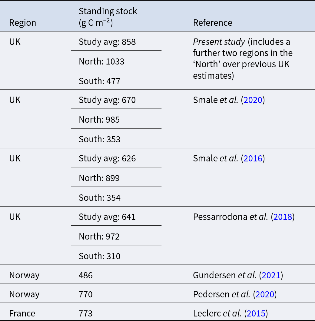
Table 4 Long description
Published estimates compare carbon standing stock for mature canopy-forming Laminaria hyperborea across regions and studies, reported in grams of carbon per square meter. Four UK studies report study averages from 626 to 858, with consistent north–south differences. In the present study, the UK average is 858, with 1033 in the North and 477 in the South. Other UK sources report North values of 899 to 985 and South values of 310 to 354, indicating northern UK forests hold roughly about two to three times the carbon of southern UK forests. Outside the UK, Norway is reported at 486 in one study and 770 in another, and France is reported at 773. Values are study means and may reflect differences in sampling locations, years, and methods, so comparisons across references should be interpreted cautiously.
Estimates reported as mean values from each study, averaged as appropriate over seasons, sites, and years. Values are for mature canopy-forming individuals only.
Estimated Laminaria hyperborea canopy carbon standing stock (g C m−2) at study sites around the United Kingdom. Bars represent mean values ± SE, n = 8–10. Points show raw data values.
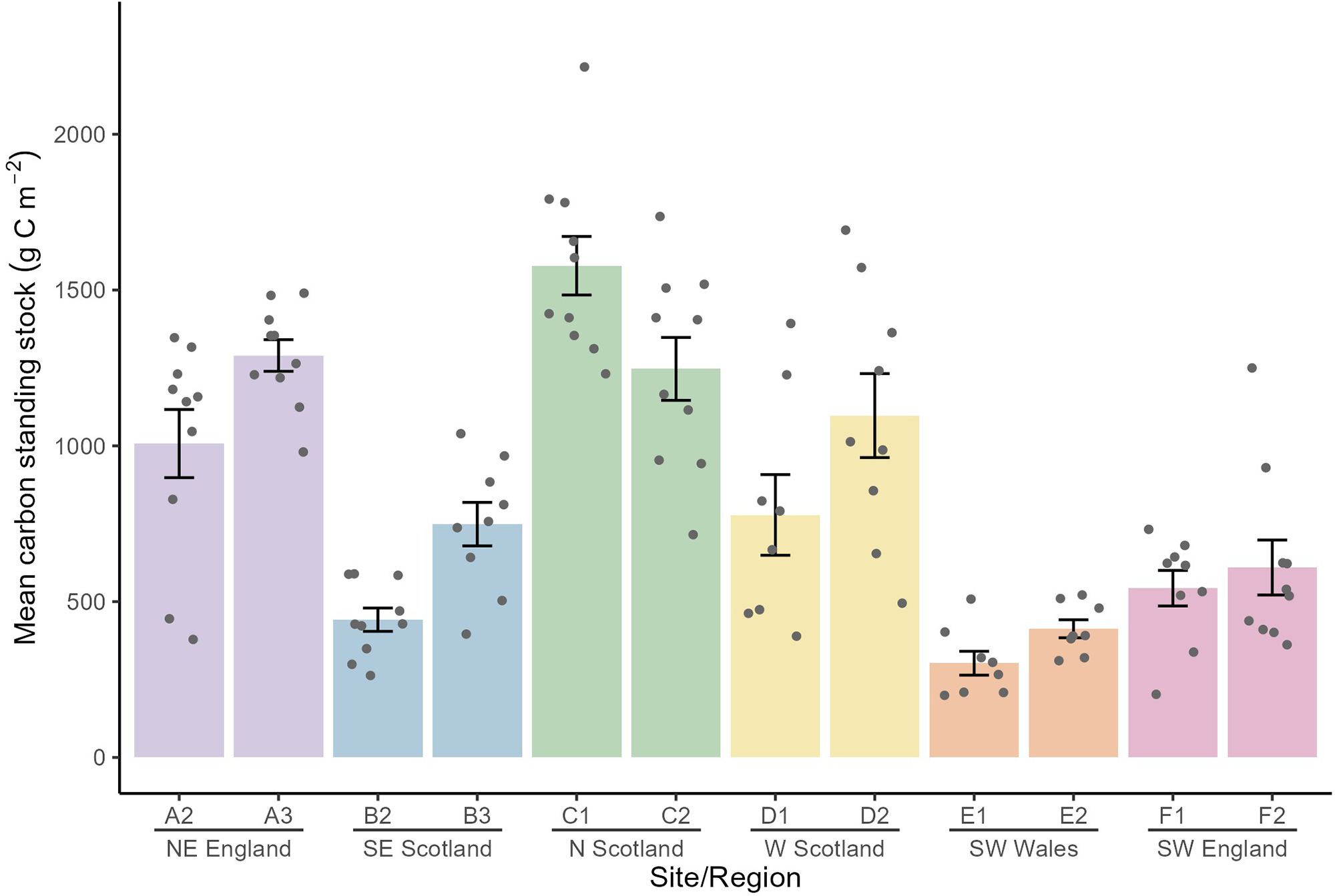
Figure 4 Long description
Bar graph with overlaid points and vertical error bars. Horizontal axis label: Site slash Region. Categories, left to right: A2, A3, B2, B3, C1, C2, D1, D2, E1, E2, F1, F2. Region labels under the categories: N E England under A2 and A3; S E Scotland under B2 and B3; N Scotland under C1 and C2; W Scotland under D1 and D2; S W Wales under E1 and E2; S W England under F1 and F2. Vertical axis label: Mean canopy carbon standing stock left parenthesis g C m superscript minus 2 right parenthesis. Tick labels shown: 0, 500, 1000, 1500, 2000. Bar heights by category: A2 about 1100; A3 about 1300; B2 about 450; B3 about 750; C1 about 1600; C2 about 1250; D1 about 800; D2 about 1100; E1 about 300; E2 about 450; F1 about 550; F2 about 600. Points are plotted above each category at multiple y values. Error bars extend above and below each bar top.
Discussion
Our results demonstrate clear spatial variability in the structure of L. hyperborea forests across NE England and SE Scotland, with individuals in NE England generally being longer and of greater biomass than those in SE Scotland. In addition, we found pronounced variability at smaller spatial scales, with sites within regions often differing markedly in density and biomass. Kelp forest structure also varied along depth gradients, with canopy density, cover, and morphological traits typically declining with depth, although site-specific deviations from this trend were observed. The morphological metrics presented in this study are used as descriptors of kelp forest structure, reflecting biological responses to local environmental conditions. These standard measures facilitate the comparison of kelp forest structure with previous studies across the geographic range of L. hyperborea.
Stipe lengths in NE England and SE Scotland were comparable to those from other UK regions (Smale et al., Reference Smale, Burrows, Evans, King, Sayer, Yunnie and Moore2016; Smale and Moore, Reference Smale and Moore2017; Smith et al., Reference Smith, Moore, King and Smale2022) and Norway (Rinde and Sjøtun, Reference Rinde and Sjøtun2005; Pedersen et al., Reference Pedersen, Nejrup, Fredriksen, Christie and Norderhaug2012; Bekkby et al., Reference Bekkby, Smit, Gundersen, Rinde, Steen, Tveiten, Gitmark, Fredriksen, Albretsen and Christie2019; Gundersen et al., Reference Gundersen, Rinde, Bekkby, Hancke, Gitmark and Christie2021) (Supplementary Table S4). In both the UK and Norway, stipe length varies along latitudinal gradients and has been linked to cooler SSTs and greater light availability in northern regions, which enhances growth (Smale et al., Reference Smale, Burrows, Evans, King, Sayer, Yunnie and Moore2016). In the UK, where L. hyperborea occurs near the centre of its distribution, stipe length generally increases with latitude (Smale et al., Reference Smale, Burrows, Evans, King, Sayer, Yunnie and Moore2016), whereas in Norway, which includes the poleward range edge, lengths increase from low to mid latitudes but decline towards higher latitudes (Gundersen et al., Reference Gundersen, Rinde, Bekkby, Hancke, Gitmark and Christie2021). These patterns suggest that L. hyperborea follows an abundant centre model (Sagarin et al., Reference Sagarin, Gaines and Gaylord2006) in terms of its population structure. Our values from the North Sea coast of the UK align with this pattern, with stipe lengths comparable to northern UK and mid-latitude Norwegian sites, where some of the longest L. hyperborea stipes are found. Although a weaker trend than for stipe length, total length also tended to increase towards northern UK regions (Smale et al., Reference Smale, Burrows, Evans, King, Sayer, Yunnie and Moore2016; Smith et al., Reference Smith, Moore, King and Smale2022). Consistent with this, we found total length in NE England and SE Scotland to be comparable to, or greater than, values reported for both UK and Norwegian populations at similar or higher latitudes, suggesting these areas represent optimal habitats for kelp growth.
Smaller L. hyperborea generally have lower biomass, and therefore trends in stipe length and biomass are often closely aligned. In the UK, canopy-forming individuals generally increase in biomass with latitude, with heavier individuals found in more northern regions (Smale et al., Reference Smale, Burrows, Evans, King, Sayer, Yunnie and Moore2016). Our results align with this pattern, with biomass values of canopy-forming kelp in SE Scotland comparable to other previously studied regions at similar latitudes (Smale et al., Reference Smale, Burrows, Evans, King, Sayer, Yunnie and Moore2016; Smith et al., Reference Smith, Moore, King and Smale2022). However, in NE England, biomass values were among some of the highest recorded for L. hyperborea, even compared to the highest UK latitudes (Smale et al., Reference Smale, Burrows, Evans, King, Sayer, Yunnie and Moore2016; Smith et al., Reference Smith, Moore, King and Smale2022) and Norway’s mid-latitudes (Gundersen et al., Reference Gundersen, Rinde, Bekkby, Hancke, Gitmark and Christie2021), regions where L. hyperborea is often found at its greatest biomass. Estimates of standing biomass, however, were considerably lower than those of Norwegian kelp forests (Gundersen et al., Reference Gundersen, Rinde, Bekkby, Hancke, Gitmark and Christie2021), yet still comparable to previous estimates from northern regions of the UK (Smale et al., Reference Smale, Burrows, Evans, King, Sayer, Yunnie and Moore2016; Smith et al., Reference Smith, Moore, King and Smale2022). Whilst no consistent latitudinal effects on kelp density have been reported, L. hyperborea populations in the UK typically occur in greater densities towards the south coast, possibly due to kelp forests being characterised by smaller individuals with lower biomasses that occupy less space, allowing a greater number of individuals to persist in a given area (Smale et al., Reference Smale, Burrows, Evans, King, Sayer, Yunnie and Moore2016; Pessarrodona et al., Reference Pessarrodona, Moore, Sayer and Smale2018). Similar patterns are reported in Norway, where the highest densities typically occur towards the northern and southern coasts, corresponding with areas where individuals are generally shorter and have lower biomass (Gundersen et al., Reference Gundersen, Rinde, Bekkby, Hancke, Gitmark and Christie2021). L. hyperborea densities in SE Scotland and NE England were generally comparable to, or greater than, other regions of similar latitude within the UK but were considerably lower than mid-latitude Norway, where densities are typically at their lowest (Pedersen et al., Reference Pedersen, Nejrup, Fredriksen, Christie and Norderhaug2012; Smale et al., Reference Smale, Burrows, Evans, King, Sayer, Yunnie and Moore2016; Gundersen et al., Reference Gundersen, Rinde, Bekkby, Hancke, Gitmark and Christie2021).
Although broad latitudinal patterns in kelp forest structure are evident, our results and those from previous studies (Smale et al., Reference Smale, Burrows, Evans, King, Sayer, Yunnie and Moore2016; Smith et al., Reference Smith, Moore, King and Smale2022) reveal pronounced variability between sites within regions. Such small-scale differences likely reflect environmental conditions that fluctuate locally as well as over large gradients, with multiple studies highlighting the role of interacting environmental drivers on small-scale variability (Pedersen et al., Reference Pedersen, Nejrup, Fredriksen, Christie and Norderhaug2012; Smale et al., Reference Smale, Burrows, Evans, King, Sayer, Yunnie and Moore2016; Smale and Moore, Reference Smale and Moore2017; Gundersen et al., Reference Gundersen, Rinde, Bekkby, Hancke, Gitmark and Christie2021; Smith et al., Reference Smith, Moore, King and Smale2022). Among these, wave exposure consistently emerges as a primary driver of kelp forest structure. In our study, greater wave fetch was associated with greater kelp biomass, density, and length, both at the site and regional levels, with individuals in NE England (where wave fetch values were greatest) significantly longer and heavier than those in SE Scotland. These patterns align with evidence that increased water movement enhances photosynthesis, nutrient uptake, and growth in L. hyperborea (Hurd, Reference Hurd2000; Pedersen et al., Reference Pedersen, Nejrup, Fredriksen, Christie and Norderhaug2012), leading to greater kelp length, biomass, and density at more exposed sites (Pedersen et al., Reference Pedersen, Nejrup, Fredriksen, Christie and Norderhaug2012; Smale et al., Reference Smale, Burrows, Evans, King, Sayer, Yunnie and Moore2016; Gundersen et al., Reference Gundersen, Rinde, Bekkby, Hancke, Gitmark and Christie2021). Such effects can be substantial, with fourfold increases in biomass and density between low- and high-exposure sites within a single region (Smale et al., Reference Smale, Burrows, Evans, King, Sayer, Yunnie and Moore2016). Indeed, such vast differences in density can be driven by an increase in sub-canopy individuals (rather than canopy-formers), which contribute little to total biomass but, importantly, serve as a critical reserve that can replace lost canopy individuals and sustain kelp forests over time (Pedersen et al., Reference Pedersen, Nejrup, Fredriksen, Christie and Norderhaug2012). Consistent with this, we found that wave fetch significantly affected total density but not the density of canopy-formers, suggesting that exposure may influence sub-canopy processes such as recruitment or competition.
Whilst wave fetch accounted for much of the site and regional scale variability in kelp forest structure, differences across depths represented a distinct and more pronounced source of variation in our study. Reductions in light availability along steep vertical gradients drive decreases in kelp productivity, growth, and density in deeper water (Sjøtun et al., Reference Sjøtun, Fredriksen and Rueness1998; Bekkby et al., Reference Bekkby, Smit, Gundersen, Rinde, Steen, Tveiten, Gitmark, Fredriksen, Albretsen and Christie2019). Not only does light penetration reduce naturally with depth, but sedimentation and turbidity can further reduce the penetrability of light, making conditions in deeper water even more challenging for autotrophic organisms (Smale and Moore, Reference Smale and Moore2017; Otero-ferrer et al., Reference Otero-ferrer, Cosme, Tuya, Espino and Haroun2020). In addition, shallower areas often benefit from greater water motion through wave action relative to deeper areas, which can increase individual movement and nutrient uptake, further promoting growth (Hurd, Reference Hurd2000; Pedersen et al., Reference Pedersen, Nejrup, Fredriksen, Christie and Norderhaug2012; Bekkby et al., Reference Bekkby, Smit, Gundersen, Rinde, Steen, Tveiten, Gitmark, Fredriksen, Albretsen and Christie2019). These processes were reflected in the patterns we observed across depth gradients in NE England and SE Scotland, where kelp forest density and cover consistently declined with depth. Biomass also tended to decrease with depth, although this pattern varied among sites. While similar depth-related declines in L. hyperborea have been documented across the UK (Smith et al., Reference Smith, Moore, King and Smale2022), the rate of reduction in biomass and density from 5 to 10 m depth was greater than previously reported at comparable UK latitudes. The structure of kelp forests beyond 5 m, as well as the depth they extend to, was most comparable to southern UK regions, where forests extend to shallower depths and are less productive than those at higher latitudes (Smale et al., Reference Smale, Burrows, Evans, King, Sayer, Yunnie and Moore2016; Smith et al., Reference Smith, Moore, King and Smale2022). Conversely, at 2 and 5 m, forests in our study were more comparable to northern populations, with kelp reaching similar lengths and densities (Smith et al., Reference Smith, Moore, King and Smale2022).
The shallower depth extent of kelp forests in our study compared to previously studied northern regions of the UK likely reflects the influence of local environmental and biological constraints, particularly light availability and grazing. Around the UK, the depth distribution of L. hyperborea varies widely, from ∼2 m in turbid areas, such as the Severn Estuary (Birkett et al., Reference Birkett, Maggs, Dring, Boaden and Seed1998) and the Yorkshire coast (Forster et al., Reference Forster, Catherall, Hull, Lecordier, Weldon, Richardson and Johnson2025), to almost 50 m in the clear waters around St Kilda (Tyler-walters, Reference Tyler-walters2007). Kelp forests in NE England and SE Scotland fall much closer to the shallow end of this spectrum, reaching a maximum depth of 13 m, and as little as 7 m. These shallow limits reflect those of southern UK regions (Smith et al., Reference Smith, Moore, King and Smale2022) and are consistent with the idea that local light availability acts as a strong control on kelp depth penetration. Local water clarity and turbidity conditions have been widely shown to constrain macroalgal depth in both the UK and beyond, with numerous examples of reductions in underwater light budgets negatively impacting depth penetration (Desmond et al., Reference Desmond, Pritchard and Hepburn2015; Tsiamis et al., Reference Tsiamis, Salomidi, Gerakaris, Mogg, Porter, Sayer and Küpper2020; Deregibus et al., Reference Deregibus, Campana, Neder, Barnes, Zacher, Piscicelli, Jerosch and Quartino2023). The presence of sea urchins in high densities has also been shown to have significant effects on the lower limit of kelp in areas of the North Atlantic, including pressure from E. esculentus in the UK (Jones and Kain, Reference Jones and Kain1967) and Strongylocentrotus droebachiensis in Iceland (Hjorleifsson et al., Reference Hjorleifsson, Kassa and Gunnarsson1995). Although grazing pressure on L. hyperborea is generally considered to be weak across much of the UK (Smale et al., Reference Smale, Burrows, Evans, King, Sayer, Yunnie and Moore2016; Hargrave et al., Reference Hargrave, Foggo, Pessarrodona and Smale2017), localised cases of elevated urchin abundance have caused reductions in kelp depth extent (Jones and Kain, Reference Jones and Kain1967; Kain and Jones, Reference Kain and Jones1977). Along the North Sea coast of the UK, urchin densities at some sites were greater than previously reported for UK kelp forests (Smale et al., Reference Smale, Burrows, Evans, King, Sayer, Yunnie and Moore2016; Smith et al., Reference Smith, Moore, King and Smale2022), reaching >4 ind. m−2, with the site with the highest urchin densities also exhibiting the shallowest kelp forest depth extent. While our data were limited and the relationship was not statistically significant, this pattern suggests that urchin grazing may contribute to restricting kelp forest depth penetration in some parts of NE England and SE Scotland. Despite this, there is currently no evidence to suggest that sea urchin grazing – which can lead to overgrazing and shifts to barren areas in other regions within this species range (Hagen, Reference Hagen1983) – has significantly impacted the structure or abundance of UK kelp forests.
This lack of grazing pressure on kelp forests in the UK suggests that the standing stock of carbon contained in L. hyperborea forests is primarily controlled by the environmental drivers that shape kelp forest structure, rather than herbivory. Consistent with previous studies (Smale et al., Reference Smale, Burrows, Evans, King, Sayer, Yunnie and Moore2016; Pessarrodona et al., Reference Pessarrodona, Moore, Sayer and Smale2018), we found higher standing stock in northern populations compared to southern areas, reflecting broad latitudinal trends linked to light availability (Smith et al., Reference Smith, Moore, King and Smale2022) and thermal stress (Allen et al., Reference Allen, Breshears and McDowell2015) that influence kelp productivity. Our study-wide mean standing stock (858 g C m−2) exceeds previous UK estimates (Table 4) and provides the first values of CSS for the North Sea coast, with NE England in particular supporting some of the highest values reported outside northern Scotland. Maximum values of standing stock (1578 g C m−2 at site C1 in N Scotland) were comparable to those previously reported in northern UK locations (Smale et al., Reference Smale, Burrows, Evans, King, Sayer, Yunnie and Moore2016, Reference Smale, Pessarrodona, King, Burrows, Yunnie, Vance and Moore2020), although variation was evident between sites within each region. However, the overall carbon stock of these kelp forests ultimately depends on their spatial extent, which remains unresolved to a fine scale and warrants further mapping.
This study establishes the first baseline of L. hyperborea forest structure and CSS along the North Sea coastline of the UK. Kelp forests in NE England and SE Scotland were found to be among the tallest recorded in the UK and exhibited some of the highest CSSs outside of northern Scotland, suggesting these regions may represent particularly favourable habitats for kelp growth. Patterns of kelp forest structure and CSS were broadly consistent with previously documented latitudinal trends, but the shallow depth limits observed here highlight the importance of local environmental and biological constraints. Considerable variability between sites within regions further emphasises the role of local-scale drivers, underlining the need to account for both regional and local processes when assessing kelp forest structure. As sampling was restricted to three sites within each of two regions, the findings should be interpreted within the spatial extent of the study and not assumed to represent kelp forest structure across the wider North Sea basin. Furthermore, because multiple response variables were analysed independently, we acknowledge that this approach increases the potential for Type I errors associated with multiple inference. However, most significant effects were supported by relatively strong statistical evidence rather than marginal p-values, and the observed patterns were generally consistent across multiple measures of kelp forest structure. Nevertheless, individual effects supported by weaker statistical evidence should be interpreted cautiously. Despite these limitations, these findings provide an important reference point for future monitoring and management of kelp forests along the North Sea coastline of the UK.
Supplementary material
The supplementary material for this article can be found at https://doi.org/10.1017/S0025315426101489.
Acknowledgements
We thank all members of ‘Team Kelp UK’ for their wider contribution to this body of work, and Dan Smale for his contribution of data from additional regions of the UK to be used in this analysis. We thank Adam Gouraguine for his assistance in the field.
Author contributions
H.C. contributed to formulating the research question, designing the study, carrying out the study, analysing the data, interpreting the findings, and writing the manuscript. H.E. contributed to carrying out the study and reviewing the draft manuscript. C.W. contributed to carrying out the study and reviewing the draft manuscript. H.S. contributed to reviewing the draft manuscript. D.S. secured funding and contributed to formulating the research question, designing the study, carrying out the study, and reviewing the draft manuscript. P.M. secured funding and contributed to formulating the research question, designing the study, carrying out the study, and reviewing the draft manuscript.
Declaration of interest
The authors declare none.
Data availability statement
Data available upon request.
Ethics and approach
No ethical considerations were needed for this research.
Funding statement
P.M., H.E., and D.S. were funded by NERC Latin America Biodiversity Fund (NE/S011692/1). D.S. is also supported by a UKRI Future Leaders Fellowship (MR/X023214/1).


 Open access

