1 Introduction
The seminal articles of Dumitrescu (Reference Dumitrescu1943) and Davies & Taylor (Reference Davies and Taylor1950) initiated a series of studies of long bubbles rising steadily in a vertical tube or channel under the effect of buoyancy. These bubbles are often referred to as gas slugs or Taylor bubbles. Liquid flows past their rounded leading tip and then falls freely in a film which may extend far downstream. In the present study, we restrict our analysis to the two-dimensional problem of a plane symmetric bubble. Interest in this geometry increased recently because the symmetry breaking observed for cylindrical bubbles in countercurrent flow (Fabre & Figueroa-Espinoza Reference Fabre and Figueroa-Espinoza2014) also occurs for plane bubbles (Figueroa-Espinoza & Fabre Reference Figueroa-Espinoza and Fabre2011), for which the two-dimensional problem is easier to tackle than the three-dimensional problem for a bubble in a tube.
Thus, we consider a symmetric plane bubble in an infinite strip of width
 $D$
. The bubble velocity
 $V$
and its shape characterized by the radius of curvature
 $R_{0}$
, where the subscript
 $0$
refers to the stagnation point, depend on the liquid density
 ${\it\rho}$
, viscosity
 ${\it\nu}$
and surface tension
 ${\it\sigma}$
, and on the acceleration due to gravity,
 $g$
. Taking
 $D/2$
and
 $\sqrt{gD}$
as the length and velocity scales, the dimensionless velocity
 $V^{\ast }=V/\sqrt{gD}$
and radius of curvature
 $R_{0}^{\ast }=2R_{0}/D$
depend on the dimensionless surface tension
 ${\it\Sigma}=4{\it\sigma}/({\it\rho}gD^{2})$
and viscosity
 $N={\it\nu}/(gD)^{3/2}$
. A comparison of earlier studies has already been presented by Figueroa-Espinoza & Fabre (Reference Figueroa-Espinoza and Fabre2011, table 1 and figure 3).
It is impossible to generate a bubble that is really two-dimensional. However, experiments in channels much wider than they are deep can approach this ideal. The first experiments mentioned in the literature (see Birkhoff & Zarantonello Reference Birkhoff and Zarantonello1957, p. 235) are probably those performed by Duff in 1927 in a
 $4^{\prime \prime }\times 1^{\prime \prime }$
vertical channel. He found that
 $V^{\ast }$
and
 $R_{0}^{\ast }$
were approximately
 $0.29$
and
 $0.70$
respectively. However, neither the flow conditions nor the experimental protocol are well documented. About four decades later, Collins (Reference Collins1965) performed careful experiments on the motion of bubbles ranging in length from spherical caps to long bubbles in a vertical rectangular channel. For long bubbles, he found
 $V^{\ast }\approx 0.25$
and
 $R_{0}^{\ast }\approx 0.62$
. The most recent experiments are probably those of Maneri & Zuber (Reference Maneri and Zuber1974), who extended their study to include inclined channels. For vertical flow they confirmed the results of Collins (Reference Collins1965). All of the above studies were carried out at negligible surface tension since
 ${\it\Sigma}$
ranged from
 $O(10^{-3})$
to
 $O(10^{-4})$
.
Numerical studies are more numerous and have usually been developed under the assumption of inviscid flow. The first to be mentioned is that of Birkhoff & Carter (Reference Birkhoff and Carter1957); although their article is mainly theoretical, the solution of their nonlinear integral equation was obtained numerically. They found
 $V^{\ast }=0.23\pm 0.01$
, but they admitted that they ‘did not get consistent predictions of
 $R_{0}^{\ast }$
’. The first fully computational study was due to Vanden-Broëck (Reference Vanden-Broëck1984a
), who solved the problem of Birkhoff & Carter (Reference Birkhoff and Carter1957) and Garabedian (Reference Garabedian1957) numerically; however, he overestimated the rise velocity by approximately
 $50\,\%$
. In a later article (Vanden-Broëck Reference Vanden-Broëck1984b
), he improved the method and included the contribution of surface tension; his results (
 $V^{\ast }=0.23$
and
 $R_{0}^{\ast }=0.64$
) closely agreed with the experiments of Maneri & Zuber (Reference Maneri and Zuber1974). Couët, Strumolo & Dukler (Reference Couët, Strumolo and Dukler1986) formulated the inviscid problem as a boundary integral of doublets. As had been shown by Garabedian (Reference Garabedian1957), they found that solutions satisfying the zero-pressure condition at the interface correspond to
 $V^{\ast }<0.35$
, and that there is a special case, corresponding to
 $V^{\ast }=0.23$
and
 $R^{\ast }=0.64$
, for which the radius of curvature varies little in the neighbourhood of the stagnation point. In a subsequent study, Couët & Strumolo (Reference Couët and Strumolo1987) extended the method to non-zero surface tension and to inclined channels. More recently, Ha Ngoc & Fabre (Reference Ha Ngoc and Fabre2006) developed a boundary element method which was used, among other tasks, for the calculation of flow around plane bubbles with surface tension in vertical, inclined and horizontal channels. They confirmed the results of Couët & Strumolo (Reference Couët and Strumolo1987). It must be stressed that most of the previous studies fit the experimental results of Maneri & Zuber (Reference Maneri and Zuber1974), thus confirming the pertinence of the inviscid assumption, at least when the dimensionless viscosity,
 $N$
, is sufficiently small. In addition to these inviscid calculations, a few direct numerical simulations should be noted: Mao & Dukler (Reference Mao and Dukler1990) computed the flow in the liquid phase with a front-tracking-like method, whereas Figueroa-Espinoza & Fabre (Reference Figueroa-Espinoza and Fabre2011) used a volume of fluid method.
In contrast to the case of cylindrical bubbles, analytical studies devoted to plane bubbles are sparse. They were all developed under the assumption of inviscid fluid. Layzer (Reference Layzer1955), motivated by astrophysical problems, assumed the form of the stream function by retaining the first term of the eigenfunction series (see appendix A). Following the method already used for cylindrical bubbles, he applied the Bernoulli condition near the stagnation point, which led him to the approximate solution of the rise velocity
 $V^{\ast }=1/\sqrt{6{\rm\pi}}=0.23$
, close to the accepted value. Garabedian (Reference Garabedian1957) derived a difference–differential equation from the Bernoulli condition at the bubble surface. He demonstrated that the flow is not uniquely determined and proposed a criterion of stability that selects the solution ‘which maximizes the velocity of the bubble’. From this criterion, he found
 $V^{\ast }=0.24$
. Collins (Reference Collins1965) investigated spherical caps to long bubbles rising in a vertical channel both experimentally and analytically. He started with an assumed stream function resulting from a doublet in a uniform flow. For a long bubble he found that the velocity is related to the radius of curvature at the stagnation point by
 $V=1/2(gR_{0})^{1/2}$
, also expressed with our scaling by
 $V^{\ast }=(R_{0}^{\ast }/8)^{1/2}$
. He also gave a radius of curvature,
 $R_{0}^{\ast }=3/{\rm\pi}=0.95$
, that overestimated his experimental result. Finally, Zudin (Reference Zudin2013) started from a stream function resulting from a source in a uniform flow. The method is similar to that of Collins (Reference Collins1965) apart from the nature of the singularity. To obtain his solution, the author had to fix the source location so that the results fitted the experiments. None of these analytical studies took account of surface tension.
2 Governing equations
For inertial flow, i.e. when the viscosity
 $N$
is small, the inviscid assumption is the right analytical framework. Because the flow is homogeneous as
 $x\rightarrow \infty$
, the stream function
 ${\it\psi}$
and the boundary conditions satisfy the Laplace equation:
 $$\begin{eqnarray}{\it\psi}_{xx}+{\it\psi}_{yy}=0,\quad ({\it\psi}_{y})_{x\rightarrow \infty }=-V,\quad ({\it\psi}_{x})_{y=\pm D/2}=0,\end{eqnarray}$$
where
 $x$
and
 $y$
are the streamwise and spanwise coordinates (see figure 1) and
 ${\it\psi}_{y}$
,
 $-{\it\psi}_{x}$
are the
 $x$
,
 $y$
components of the velocity vector. If we assume constant pressure inside the bubble, the Bernoulli condition at the bubble surface becomes
 $$\begin{eqnarray}\frac{1}{2}\left({\it\psi}_{x}^{2}+{\it\psi}_{y}^{2}\right)+gx-\frac{{\it\sigma}}{{\it\rho}}\left(R^{-1}-R_{0}^{-1}\right)=0.\end{eqnarray}$$
Written in dimensionless form, the Laplace equation takes the same form as (2.1), whereas the Bernoulli condition becomes
 $$\begin{eqnarray}b^{\ast }(x^{\ast },y^{\ast }):=\left({\it\psi}_{x^{\ast }}^{\ast 2}+{\it\psi}_{y^{\ast }}^{\ast 2}\right)+x^{\ast }-{\it\Sigma}\left(R^{\ast -1}-R_{0}^{\ast -1}\right)=0.\end{eqnarray}$$
For simplicity, stars will be dropped from dimensionless quantities hereafter.
The starting point of the method is to conjecture the form of the stream function. A truncated series of eigenfunctions could be used, but the resulting accuracy would be far from satisfactory. Indeed, if the rise velocity agrees with the experimental results, the radius of curvature at the tip and thus the bubble shape are poorly predicted (see appendix A). Other previous studies have considered the superposition of a uniform flow and the flow induced by a singularity: a doublet was chosen by Collins (Reference Collins1965) and a source by Zudin (Reference Zudin2013). While a doublet is convenient for the closed surface of a bubble of limited extent, a source is more adapted to the quasi-open surface of a long bubble. Here, we adopt for
 ${\it\psi}$
the superposition of a uniform flow and the flow induced by a source. The complex potential of a source in the unit strip, located at the origin, is given by Lamb (Reference Lamb1945, p. 71). The stream function resulting from a source located at
 $x={\it\xi}({<}0)$
and a uniform flow of velocity
 $-V$
at
 $x\rightarrow \infty$
takes the form
 $$\begin{eqnarray}{\it\psi}=V\left\{\frac{1}{{\rm\pi}}(1-\text{e}^{-{\rm\pi}{\it\xi}})\tan ^{-1}\left[\tan \left(\frac{{\rm\pi}y}{2}\right)\coth \left(\frac{{\rm\pi}({\it\xi}-x)}{2}\right)\right]-\frac{1}{2}\left(1+\text{e}^{-{\rm\pi}{\it\xi}}\right)y\right\},\end{eqnarray}$$
where the source intensity and position are chosen for the stagnation point to be at the origin (
 ${\it\psi}_{y}(0,0)=0$
) and where the stream function is such that
 ${\it\psi}(0,0)=0$
. It should be noted that
 ${\it\psi}$
and all of its derivatives with respect to
 $x$
and/or
 $y$
are linear functions of
 $V$
.
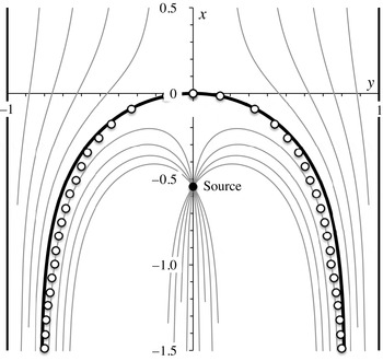
Sketch of the flow induced by a source located at
 $x=-0.545$
for
 ${\it\Sigma}=0$
. Bubble shape from (2.5), thick solid lines; streamlines from (2.7), thin solid lines; results of Maneri & Zuber (Reference Maneri and Zuber1974), circles.

The implicit form
 ${\it\psi}(x,y)=0$
of the interface equation can be put into the explicit form
 $x=X(y)$
:
 $$\begin{eqnarray}X={\it\xi}-\frac{2}{{\rm\pi}}\tanh ^{-1}\left\{\tan \left(\frac{{\rm\pi}y}{2}\right)\cot \left[\frac{{\rm\pi}y}{2}\coth \left(\frac{{\rm\pi}{\it\xi}}{2}\right)\right]\right\}.\end{eqnarray}$$
The radius of curvature at the bubble tip can be expressed from (2.5) as
 $$\begin{eqnarray}R_{0}=-\frac{3}{{\rm\pi}}\tanh \left(\frac{{\rm\pi}{\it\xi}}{2}\right).\end{eqnarray}$$
Equations (2.5) and (2.6) show that if we know the source location,
 ${\it\xi}$
, the bubble shape is fully determined. It should be noted that the same is true for the bubble velocity. Finally, the explicit equation for the streamlines is an extension of (2.5):
 $$\begin{eqnarray}X_{{\it\psi}}={\it\xi}-\frac{2}{{\rm\pi}}\tanh ^{-1}\left\{\tan \left(\frac{{\rm\pi}y}{2}\right)\cot \left[\frac{{\rm\pi}}{2}\left((y+{\it\psi}/V)\coth \left(\frac{{\rm\pi}{\it\xi}}{2}\right)+{\it\psi}/V\right)\right]\right\},\end{eqnarray}$$
where
 ${\it\psi}/V\in [-1,1]$
. An example of the streamlines is shown in figure 1 for
 ${\it\Sigma}=0$
.
The Bernoulli condition (2.3) must be fulfilled at the interface:
 $b[X(y),y]=0$
. Because the form of the interface is given, it is impossible to satisfy this condition everywhere on (2.5). Here, we restrict the Bernoulli condition to the vicinity of the stagnation point. If
 $b[X(y),y]$
is expressed by a Taylor series about this point, the condition is equivalent to ensuring that all derivatives of
 $b$
with respect to
 $y$
at
 $y=0$
, i.e.
 $b_{0}^{\prime },b_{0}^{\prime \prime },b_{0}^{(3)}$
etc., are zero. Because the odd derivatives at this point are zero by symmetry, the first non-trivial condition is
 $b_{0}^{\prime \prime }=0$
:
 $$\begin{eqnarray}15\left[{\it\psi}_{xy}^{2}\left(6{\it\psi}_{xy}^{3}-{\it\psi}_{yyy}\right)\right]_{0}+{\it\Sigma}\left[20{\it\psi}_{yyy}^{3}+30{\it\psi}_{xy}{\it\psi}_{xyyy}{\it\psi}_{yyy}-9{\it\psi}_{yyyyy}{\it\psi}_{xy}^{2}\right]_{0}=0.\end{eqnarray}$$
More effort is needed to express the second condition,
 $b_{0}^{(4)}=0$
:
 $$\begin{eqnarray}\displaystyle & & \displaystyle \left[120{\it\psi}_{xyyy}{\it\psi}_{xy}^{4}+160{\it\psi}_{yyy}^{2}{\it\psi}_{xy}^{3}-3{\it\psi}_{yyyyy}{\it\psi}_{xy}^{2}+10{\it\psi}_{yyy}{\it\psi}_{xyyy}{\it\psi}_{xy}+5{\it\psi}_{yyy}^{3}\right]_{0}\nonumber\\ \displaystyle & & \displaystyle \quad -\,\frac{5{\it\Sigma}}{63({\it\psi}_{xy}^{2})_{0}}\left[560{\it\psi}_{yyy}^{5}+1470{\it\psi}_{xy}{\it\psi}_{xyyy}{\it\psi}_{yyy}^{3}+630{\it\psi}_{xy}^{2}{\it\psi}_{yyy}({\it\psi}_{xyyy}^{2}-{\it\psi}_{yyyyy}{\it\psi}_{yyy})\right.\nonumber\\ \displaystyle & & \displaystyle \left.\quad -\,189{\it\psi}_{xy}^{3}({\it\psi}_{xyyyyy}{\it\psi}_{yyy}+{\it\psi}_{yyyyy}{\it\psi}_{xyyy})+27{\it\psi}_{yyyyyyy}{\it\psi}_{xy}^{4}\right]_{0}=0.\end{eqnarray}$$
It should be noted that (2.8) and (2.9) simplify by using
 ${\it\psi}_{xx}=-{\it\psi}_{yy}$
. These equations are independent of the form of the stream function and therefore they can be used with other forms of symmetric stream functions in potential flow.
3 Solution for zero surface tension (
 ${\it\Sigma}=0$
)

The Bernoulli conditions (2.8) and (2.9) greatly simplify when
 ${\it\Sigma}=0$
. Applied to the stream function (2.4), the condition (2.8) becomes
 $$\begin{eqnarray}{\it\Xi}^{2}+6{\rm\pi}V^{2}-1=0,\end{eqnarray}$$
where we put
 ${\it\Xi}=\text{e}^{{\rm\pi}{\it\xi}}$
. The resulting solution for
 $V$
depends on
 ${\it\Xi}$
, so that the next condition,
 $b_{0}^{(4)}=0$
, is needed to fix the source coordinate. Equation (2.9) becomes
 $$\begin{eqnarray}{\it\Xi}^{4}+20{\rm\pi}\left({\it\Xi}^{2}-4{\it\Xi}+1\right)V^{2}-1=0.\end{eqnarray}$$
These two algebraic equations can be easily solved by eliminating
 $V^{2}$
. Then, the pertinent solution, i.e. the one that leads to a positive value of
 $V$
, is
 $$\begin{eqnarray}{\it\Xi}=\text{e}^{{\rm\pi}{\it\xi}}=\frac{1}{7}(20-3\sqrt{39}),\quad V=\frac{1}{7}\sqrt{\frac{20\sqrt{39}-117}{{\rm\pi}}},\quad R_{0}=\frac{1}{{\rm\pi}}\sqrt{\frac{13}{3}},\end{eqnarray}$$
i.e.
 ${\it\xi}=-0.55$
,
 $V=0.23$
and
 $R_{0}=0.66$
.
The velocity and the radius of curvature are in close agreement with the inviscid numerical simulations of Vanden-Broëck (Reference Vanden-Broëck1984b
) and Ha Ngoc & Fabre (Reference Ha Ngoc and Fabre2004) and with the direct numerical simulations of Mao & Dukler (Reference Mao and Dukler1990). Although the velocity is slightly underestimated with respect to the experiments of Maneri & Zuber (Reference Maneri and Zuber1974), this is also true for most numerical studies, suggesting that the three-dimensional character of the experimental channel could be an issue. The present method works well in predicting the bubble shape: figure 1 shows that (2.5) and the shape of Maneri & Zuber (Reference Maneri and Zuber1974) fully agree. The streamlines given by (2.7) for
 ${\it\Sigma}=0$
are also plotted in figure 1.
4 Solution with surface tension (
${\it\Sigma}>0$
)

For
 ${\it\Sigma}>0$
the two conditions (2.8) and (2.9) become
 $$\begin{eqnarray}15({\it\Xi}-1)\left({\it\Xi}^{2}+6{\rm\pi}V^{2}-1\right)+{\rm\pi}^{2}({\it\Xi}+1)({\it\Xi}^{2}-10{\it\Xi}+1){\it\Sigma}=0\end{eqnarray}$$
and
 $$\begin{eqnarray}\displaystyle & & \displaystyle 126({\it\Xi}-1)\left[{\it\Xi}^{4}+20{\rm\pi}\left({\it\Xi}^{2}-4{\it\Xi}+1\right)V^{2}-1\right]\nonumber\\ \displaystyle & & \displaystyle \quad -\,5{\rm\pi}^{2}({\it\Xi}+1)\left({\it\Xi}^{4}+28{\it\Xi}^{3}-90{\it\Xi}^{2}+28{\it\Xi}+1\right){\it\Sigma}=0.\end{eqnarray}$$
Eliminating
 $V^{2}$
between (4.1) and (4.2) leads to
 $$\begin{eqnarray}{\it\Sigma}=-\frac{14(1-{\it\Xi})^{2}\left(7-40{\it\Xi}+7{\it\Xi}^{2}\right)}{{\rm\pi}^{2}\left(11-84{\it\Xi}+242{\it\Xi}^{2}-84{\it\Xi}^{3}+11{\it\Xi}^{4}\right)}.\end{eqnarray}$$
The radius of curvature is expressed from (2.6) as
 $$\begin{eqnarray}R_{0}=\left(\frac{3}{{\rm\pi}}\right)\frac{1-{\it\Xi}}{1+{\it\Xi}}.\end{eqnarray}$$
Finally, the rise velocity is obtained by combining (4.1) and (4.3):
 $$\begin{eqnarray}V=\sqrt{\frac{(1-{\it\Xi}^{2})\left(67+280{\it\Xi}-2166{\it\Xi}^{2}+280{\it\Xi}^{3}+67{\it\Xi}^{4}\right)}{90{\rm\pi}\left(11-84{\it\Xi}+242{\it\Xi}^{2}-84{\it\Xi}^{3}+11{\it\Xi}^{4}\right)}}.\end{eqnarray}$$
The terms
 $R_{0}({\it\Sigma})$
and
 $V({\it\Sigma})$
are obtained as functions of
 ${\it\Sigma}$
by use of (4.3).


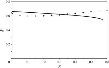
Radius of curvature
 $R_{0}$
. Present model, solid line; Maneri & Zuber (Reference Maneri and Zuber1974), circle; Ha Ngoc & Fabre (Reference Ha Ngoc and Fabre2004), crosses.

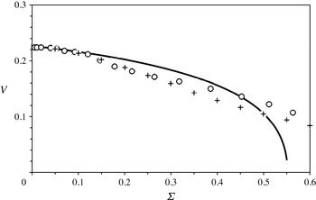
Bubble velocity
 $V$
. Present model, solid line. Numerical simulations: Ha Ngoc & Fabre (Reference Ha Ngoc and Fabre2004), crosses; Couët & Strumolo (Reference Couët and Strumolo1987), circles.

The source position
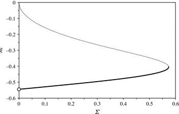
 ${\it\xi}=1/{\rm\pi}\log ({\it\Xi})$
is plotted in figure 2. There are two solutions for
 ${\it\xi}({\it\Sigma})$
if
 $0<{\it\Sigma}<{\it\Sigma}_{M}$
, and no solution for
 ${\it\Sigma}>{\it\Sigma}_{M}=7\left(27\sqrt{10}-19\right)/(82{\rm\pi}^{2})\approx 0.574$
. The physical solution, which matches (3.3) for
 ${\it\Sigma}=0$
, corresponds to the lower branch of figure 2: the distance of the source location to the stagnation point decreases almost linearly with
 ${\it\Sigma}$
. The radius of curvature is plotted in figure 3, and the bubble velocity in figure 4. Except for very small
 ${\it\Sigma}$
(i.e. Maneri & Zuber Reference Maneri and Zuber1974), no experimental results are available. Only the numerical results of Couët & Strumolo (Reference Couët and Strumolo1987) and Ha Ngoc & Fabre (Reference Ha Ngoc and Fabre2004) cover a range of surface tension wide enough to assess the model. The radius of curvature
 $R_{0}$
, given by (4.4), slightly decreases when
 ${\it\Sigma}$
increases, whereas Ha Ngoc & Fabre (Reference Ha Ngoc and Fabre2004) predict that it remains almost constant. The bubble velocity
 $V$
decreases when
 ${\it\Sigma}$
increases, suggesting that surface tension acts as a resisting force opposed to gravity; the agreement between our results and those of Ha Ngoc & Fabre (Reference Ha Ngoc and Fabre2004) and Couët & Strumolo (Reference Couët and Strumolo1987) is excellent for
 ${\it\Sigma}<0.15$
. For higher
 ${\it\Sigma}$
there are discrepancies which become important for
 ${\it\Sigma}>0.5$
. In particular, the present theory predicts that the bubble velocity becomes zero for
 ${\it\Sigma}=(\sqrt{193}-3)/(2{\rm\pi}^{2})\approx 0.55$
, whereas the numerical solutions suggest that this might occur only at some larger value of
 ${\it\Sigma}$
.
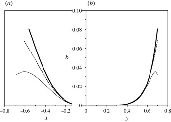
Deviation from the Bernoulli condition at the interface, versus
 $x$
(a) or
 $y$
(b):
 ${\it\Sigma}=0$
, thick solid line;
 ${\it\Sigma}=0.20$
, dotted line;
 ${\it\Sigma}=0.4$
, thin solid line.

To check the accuracy to which the Bernoulli condition is satisfied we calculated
 $b[X(y),y]$
, which should be zero along the interface. The results are shown in figure 5 for three different values of the surface tension. The deviation of
 $b$
from zero is smaller than
 $0.01$
for
 $y\lessapprox 0.55$
and for
 $|x|\lessapprox 0.25$
.
5 Conclusion
The present article is a contribution to our understanding of the dynamics and shape of a plane bubble rising steadily in a channel under the influence of buoyancy. In the framework of inviscid theory, we developed an analytical model that includes surface tension effects. The stream function is assumed to be a superposition of the potential flows of a uniform stream and a source in the unit strip. The Bernoulli equation at the interface is satisfied up to fourth order in a Taylor expansion in the neighbourhood of the stagnation point. The present model gives the rise velocity with an accuracy probably better than previously, especially for
 ${\it\Sigma}<0.15$
, and provides an analytical expression for the bubble shape. Although plane bubbles are of theoretical (rather than practical) interest, the existence of an analytical solution for the flow field is a potentially useful step for future studies of bubble stability.
Appendix A. Solutions from truncated series of eigenfunctions
The generalized form of the Layzer (Reference Layzer1955) stream function for a uniform flow of velocity
 $-V$
in the strip
 $y\in [-1,+1]$
is given as a truncated order-
 $n$
series of eigenfunctions:
 $$\begin{eqnarray}{\it\psi}=-Vy+\mathop{\sum }_{k=1}^{n}c_{k}\text{e}^{-k{\rm\pi}x}\sin (k{\rm\pi}y).\end{eqnarray}$$
For practical purposes it is desirable to use as few terms in the series as possible. We show here that when
 $n=1$
the series is insufficiently accurate, and an increase in the number of terms to
 $n>1$
complicates the solution with only marginal improvement in accuracy.
With only the first term of the series (
 $n=1$
) and the first Bernoulli condition (2.8), one finds
 $c_{1}=1/{\rm\pi}\sqrt{6{\rm\pi}}$
. The bubble velocity, the radius of curvature at the stagnation point and the shape equation become
 $$\begin{eqnarray}V=\sqrt{\frac{1+\frac{1}{15}{\it\Sigma}}{6{\rm\pi}}},\quad R_{0}=\frac{3}{{\rm\pi}},\quad X=\frac{1}{{\rm\pi}}\log \left[\frac{\sin ({\rm\pi}y)}{{\rm\pi}y}\right],\end{eqnarray}$$
i.e.
 $V=0.23+\sqrt{1+0.658{\it\Sigma}}$
and
 $R_{0}=0.955$
. Not only is the radius of curvature overestimated but the velocity increases with
 ${\it\Sigma}$
, which it should not.
With the first two terms of the series (
 $n=2$
) and the two Bernoulli conditions (2.8) and (2.9), the results are worse. For example, for
 ${\it\Sigma}=0$
we found
 $c_{1}=0.0702$
and
 $c_{2}=-0.0070$
, leading to
 $V=0.176$
and
 $R_{0}=2.91$
.
Only with the first two odd terms of the series (
 $k=1,3$
) together with the two Bernoulli conditions (2.8) and (2.9) are the results acceptable. Indeed, for
 ${\it\Sigma}=0$
we found
 $c_{1}=0.0719$
and
 $c_{3}=0.00105$
, leading to
 $V=0.236$
and
 $R_{0}=0.775$
.
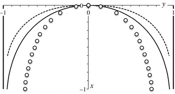
Results for the bubble shape are shown in figure 6. With the assumed form (A 1) the truncated series is accurate for neither
 $n=1$
nor
 $n=2$
. Calculations for
 $n=3$
together with an additional Bernoulli condition (
 $b_{0}^{(6)=0}$
) show that, if the shape improves near the stagnation point, it deteriorates far from it.
Bubble shape for
 ${\it\Sigma}=0$
. Solution (A 1) for
 $n=1$
: solid line and for
 $n=2$
: dotted line. Experimental results of Maneri & Zuber (Reference Maneri and Zuber1974): circles.