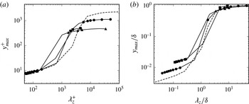
1. Introduction
Since the pioneering study of Theodorsen (Reference Theodorsen1952) on horseshoe vortices, it has been known that coherent motions play a major role in the dynamics of wall turbulence. According to the mechanism proposed by Hamilton, Kim & Waleffe (Reference Hamilton, Kim and Waleffe1995) and later confirmed by the numerical experiment of Jiménez & Pinelli (Reference Jiménez and Pinelli1999), near-wall turbulence is characterized by a self-sustaining process, which relies on the formation and the subsequent breakdown of streamwise velocity streaks. The streaks, having a characteristic spanwise spacing of approximately 100 wall units (Kline et al. Reference Kline, Reynolds, Schraub and Runstadler1967), are induced by the advection of the mean velocity field by quasi-streamwise vortices, which are in turn generated by streak instability. While the dynamics and the typical structures of the near-wall layer are sufficiently well understood, much less is known about the structure of the outer layer, which has been the focus of substantial research in the past years. Recent experiments and numerical studies have revealed the existence of very long, meandering features consisting of regions of low-streamwise-momentum fluid flanked by higher-momentum fluid, commonly referred to as large- and very-large-scale motions (LSM, VLSM) in internal flows, and as superstructures in external flows (Smits, McKeon & Marusic Reference Smits, McKeon and Marusic2011). According to Kim & Adrian (Reference Kim and Adrian1999), these motions are created by the organization of vortices into packets, formed by multiple hairpin vortices travelling at the same velocity.
The study of the spatial and temporal scales of coherent structures, and of their mutual interactions, is fundamental for developing low-order models of wall turbulence (Panton Reference Panton2001). In this context, although turbulence requires the nonlinearity of the Navier–Stokes equations, there is strong evidence that the emergence of coherent structures and energy production mechanisms can be described through linear models (Jiménez Reference Jiménez2013). For laminar shear flows, Schmid & Henningson (Reference Schmid and Henningson2001) have shown that linear stability theory based on transient growth provides some understanding of the early stages of amplification of the streaks. In the case of wall-bounded turbulent shear flows, Butler & Farrel (Reference Butler and Farrel1992) carried out an optimal transient growth analysis by linearizing the Navier–Stokes equations about the mean flow, and modelling the effect of the small-scale turbulence on the coherent part of motion by constraining the optimization time with the eddy turnover time. They showed that the most amplified modes have a characteristic spanwise wavelength of
 $O(100)$
wall units, thus matching the spacing of streaks observed in experiments (Kim, Kline & Reynolds Reference Kim, Kline and Reynolds1971).
The importance of linear processes in the sustainment of near-wall turbulence in channel flow has been numerically investigated by Kim & Lim (Reference Kim and Lim2000). By setting to zero the linear coupling term representing the transfer from wall-normal velocity to wall-normal vorticity, those authors showed suppression of linear transient growth, with subsequent strong reduction of turbulence, and disappearance of the streamwise vortices. They then concluded that, although near-wall turbulence features nonlinear processes (bursting events being an example), its maintenance relies on linear processes of transient growth. Other evidence for the importance of linear processes has been recently given by Alizard, Robinet & Filliard (Reference Alizard, Robinet and Filliard2015), who developed a linear theory for the control of incompressible near-wall turbulence.
The temporal stability of the Orr–Sommerfeld and Squire equations in channels with turbulent mean velocity profiles and turbulent eddy viscosities was studied by del Alamo & Jiménez (Reference del Alamo and Jiménez2006), who, using a linear transient growth analysis, identified two maxima, one corresponding to the sublayer streaks and the other to large-scale global structures spanning the full channel. In the intermediate region, the authors also remark that the maximum gain reaches an almost constant value and the corresponding modes exhibit self-similarities, in agreement with the observed structures in the logarithmic layer. Similar results were obtained by Pujals et al. (Reference Pujals, Garci-Villalba, Cossu and Depardon2009), who also found that the optimal growth rate in the outer region varies linearly with a turbulent Reynolds number based on the maximum velocity, the channel half-width and the maximum eddy viscosity. Optimal transient growth in incompressible turbulent boundary layers was studied by Cossu, Pujals & Depardon (Reference Cossu, Pujals and Depardon2009). Using an analytical mean flow and the eddy viscosity model of Monkewitz, Chauhan & Nagib (Reference Monkewitz, Chauhan and Nagib2007), they showed that a double-peak structure of the optimal energy gain characterizes the organized turbulence dynamics.
In particular, in the near-wall region, streaky structures scale in wall units and are independent of the Reynolds number, while away from the wall they scale in outer units, and the optimal gain varies with the Reynolds number. They also found close similarity of the flow topology with data from direct numerical simulation (DNS) and experiments, thus confirming the effectiveness of optimal transient growth analysis in describing the initial stages of nonlinear processes of turbulence self-sustainment. However, as Cossu et al. (Reference Cossu, Pujals and Depardon2009) pointed out, transient growth analysis may fail to yield quantitatively correct spanwise and streamwise wavelengths of the outer-layer structures.
The focus of the present study is on compressible wall-bounded turbulence. Early studies of compressible wall-bounded flows have led to the widely accepted notion that the main effect of flow compressibility resides in the incurred mean density variations, which can be compensated through suitable transformations to recover the incompressible statistics (Morkovin Reference Morkovin and Favre1961). In general terms, the essential topology of the coherent structures is also believed to be very similar, and streaks and hairpins have been observed in experiments and DNS of supersonic boundary layers (Spina, Smits & Robinson Reference Spina, Smits and Robinson1994; Smith & Smits Reference Smith and Smits1995; Ringuette, Wu & Martín Reference Ringuette, Wu and Martín2008; Pirozzoli, Bernardini & Grasso Reference Pirozzoli, Bernardini and Grasso2008, Reference Pirozzoli, Bernardini and Grasso2010; Elsinga et al. Reference Elsinga, Adrian, van Oudheusden and Scarano2010). Sufficiently high Reynolds numbers to observe the emergence of superstructures and the formation of a genuine logarithmic layer have recently been attained in DNS (Pirozzoli & Bernardini Reference Pirozzoli and Bernardini2011, Reference Pirozzoli and Bernardini2013). These studies have shown that the interaction mechanisms occurring between the large-scale motions of the outer layer and the near-wall streaks are similar to those of the incompressible regime and are characterized by phenomena of imprinting and amplitude modulation (Bernardini & Pirozzoli Reference Bernardini and Pirozzoli2011a ). The results of Lagha et al. (Reference Lagha, Kim, Eldredge and Zhong2011) further confirmed that supersonic and hypersonic turbulent boundary layers have close similarities with incompressible boundary layers, when accounting for the effect of mean density variations. In particular, consistent with the results of Kim & Lim (Reference Kim and Lim2000), they showed that if the linear coupling term is removed, near-wall turbulence cannot be sustained, thus indicating that linear transient growth plays an important role also in the compressible flow regime.
The experimental and theoretical evidence for the similarity between incompressible and compressible coherent structures, and their role in the wall-turbulence dynamics, have led us to develop a theoretical analysis of optimal transient growth, by extending to compressible flows the triple decomposition approach originally developed by Reynolds & Hussain (Reference Reynolds and Hussain1972) for low-speed flows, whereby the instantaneous flow field is separated into the contributions of mean flow, organized and background disorganized turbulent motions.
The main goal of this work is to highlight the physical mechanisms associated with the formation of coherent structures in compressible boundary layers, thus addressing fundamental questions such as the following: (i) Do compressible turbulent boundary layers exhibit a double peak in the optimal energy growth? (ii) Does the spatial and temporal scale selection mechanism obey inner and outer scaling? (iii) What are the effects associated with flow compressibility on the energy budget of optimal modes and on the vorticity transfer mechanism in the inner and outer regions? (iv) How does the compressibility affect modes that populate the logarithmic region?
The paper is organized as follows. In § 2 we formulate the governing equations based on triple decomposition adapted to compressible turbulent flows, and discuss the closure for turbulent transport of momentum and energy associated with the coherent motions in boundary layers. In § 3 we develop the optimal energy growth analysis for the inner and the outer part of the boundary layer, including the energy budget and the vorticity transfer mechanism, and analyse the influence of the Mach number. Section 4 is devoted to drawing conclusions and perspectives.
2. Analysis of coherent motions
2.1. Governing equations
The Navier–Stokes equations for a compressible perfect gas are
 $$\begin{eqnarray}\displaystyle & \displaystyle \frac{\partial {\it\rho}}{\partial t}+\frac{\partial }{\partial x_{j}}({\it\rho}u_{j})=0, & \displaystyle\end{eqnarray}$$
 $$\begin{eqnarray}\displaystyle & \displaystyle \frac{\partial }{\partial t}({\it\rho}u_{i})+\frac{\partial }{\partial x_{j}}({\it\rho}u_{i}u_{j})=-\frac{\partial }{\partial x_{i}}p+\frac{\partial }{\partial x_{j}}{\it\sigma}_{ij}, & \displaystyle\end{eqnarray}$$
 $$\begin{eqnarray}\displaystyle & \displaystyle \frac{\partial }{\partial t}({\it\rho}e)+\frac{\partial }{\partial x_{j}}({\it\rho}eu_{j})=-\frac{\partial }{\partial x_{j}}{\it\psi}_{j}+{\it\sigma}_{ij}\frac{\partial u_{i}}{\partial x_{j}}-p\frac{\partial u_{i}}{\partial x_{i}}, & \displaystyle\end{eqnarray}$$
 ${\it\rho},~p,~u_{i}$
and
 $e$
are, respectively, density, pressure, the
 $i$
th velocity component and internal energy. The viscous stress tensor
 $({\it\sigma}_{ij})$
and the heat flux vector
 $({\it\psi}_{j})$
components are defined as
 $$\begin{eqnarray}\left.\begin{array}{@{}l@{}}\displaystyle {\it\sigma}_{ij}={\it\mu}(T)\left(\frac{\partial u_{i}}{\partial x_{j}}+\frac{\partial u_{j}}{\partial x_{i}}\right)-\frac{2}{3}{\it\mu}(T){\it\delta}_{ij}\frac{\partial u_{k}}{\partial x_{k}},\\ \displaystyle {\it\psi}_{j}=-\frac{c_{p}{\it\mu}(T)}{\mathit{Pr}}\frac{\partial T}{\partial x_{j}},\end{array}\right\}\end{eqnarray}$$
where
 ${\it\delta}_{ij}$
,
 $\mathit{Pr}$
and
 ${\it\mu}(T)$
are Kronecker’s delta, the Prandtl number and the molecular viscosity (the latter is defined by assuming Sutherland’s law). The temperature is defined as
 $T=e/c_{v}$
, and
 $c_{p}$
and
 $c_{v}$
are the specific heat at constant pressure and constant volume, respectively.
To study coherent motions in incompressible turbulent shear flows, Reynolds & Hussain (Reference Reynolds and Hussain1972) introduced a triple decomposition of the instantaneous fields into mean flow, organized motions and small-scale random motions. Hence, any variable
 ${\it\phi}$
is decomposed as
 $$\begin{eqnarray}{\it\phi}=\overline{{\it\phi}}+{\it\phi}^{\prime ,\ell }+{\it\phi}^{\prime ,t},\end{eqnarray}$$
where
 $\overline{(\cdot )}$
,
 $(\cdot )^{\prime ,\ell }$
and
 ${(\cdot )^{\prime }}^{,t}$
represent, respectively, the long-time average, the contribution associated with organized motions and the random contribution due to the small scales. The coherent part is extracted from the instantaneous flow by phase averaging
 $(\langle \cdot \rangle )$
, and by assuming that the coherent and the random contributions are decorrelated with respect to time and phase, thus having
 $$\begin{eqnarray}{\it\phi}^{\prime ,\ell }=\langle {\it\phi}\rangle -\overline{{\it\phi}},\quad {\it\phi}^{\prime ,t}={\it\phi}-\langle {\it\phi}\rangle .\end{eqnarray}$$
Here we apply the incompressible triple decomposition to the density and the pressure fields, and introduce a mass-weighted triple decomposition for the velocity and the temperature fields
 $$\begin{eqnarray}{\it\phi}=\tilde{{\it\phi}}+{\it\phi}^{\prime \prime ,\ell }+{\it\phi}^{\prime \prime ,t},\end{eqnarray}$$
where
 ${\it\phi}$
stands for either velocity or temperature. Here
 $\tilde{{\it\phi}}$
,
 ${\it\phi}^{\prime \prime ,\ell }$
and
 ${\it\phi}^{\prime \prime ,t}$
represent, respectively, the mass-weighted time average, and the contributions of the coherent and incoherent motions evolving about the density-weighted mean flow. In the framework of mass averaging, in order to be decorrelated with respect to both time and phase, the organized and the random parts are defined as
 $$\begin{eqnarray}{\it\phi}^{\prime \prime ,\ell }=\frac{\langle {\it\rho}{\it\phi}\rangle }{\langle {\it\rho}\rangle }-\tilde{{\it\phi}},\quad {\it\phi}^{\prime \prime ,t}={\it\phi}-\frac{\langle {\it\rho}{\it\phi}\rangle }{\langle {\it\rho}\rangle }.\end{eqnarray}$$
The equations governing the coherent dynamics are then obtained by applying the above triple decompositions to (2.1)–(2.3), after phase averaging and subtracting the time average:
 $$\begin{eqnarray}\displaystyle \frac{\partial }{\partial t}{\it\rho}^{\prime ,\ell }+\frac{\partial }{\partial x_{k}}\mathscr{J}_{k}^{\ell }=0, & & \displaystyle\end{eqnarray}$$
 $$\begin{eqnarray}\displaystyle & & \displaystyle \displaystyle \frac{\partial }{\partial t}(\langle {\it\rho}\rangle u_{i}^{\prime \prime ,\ell })+\frac{\partial }{\partial x_{k}}(\langle {\it\rho}\rangle \widetilde{u_{k}}u_{i}^{\prime \prime ,\ell })+\mathscr{J}_{k}^{\ell }\frac{\partial \widetilde{u_{i}}}{\partial x_{k}}\nonumber\\ \displaystyle & & \displaystyle \quad =-\frac{\partial }{\partial x_{i}}p^{\prime ,\ell }+\frac{\partial }{\partial x_{k}}{\it\sigma}_{ik}^{\prime \prime ,\ell }-\frac{\partial }{\partial x_{k}}\left[(\langle r_{ik}^{\ell }\rangle +\langle r_{ik}^{t}\rangle )-\left(\overline{r_{ik}^{\ell }}+\overline{r_{ik}^{t}}\right)\right]+\mathscr{H}_{u_{i}},\end{eqnarray}$$
 $$\begin{eqnarray}\displaystyle & & \displaystyle \displaystyle \frac{\partial }{\partial t}(\langle {\it\rho}\rangle \text{e}^{\prime \prime ,\ell })+\frac{\partial }{\partial x_{k}}(\langle {\it\rho}\rangle \widetilde{u_{k}}\text{e}^{\prime \prime ,\ell })+\mathscr{J}_{k}^{\ell }\frac{\partial \widetilde{e}}{\partial x_{k}}\nonumber\\ \displaystyle & & \displaystyle \quad =-\frac{\partial {\it\psi}_{k}^{\prime \prime ,\ell }}{\partial x_{k}}-\frac{\partial }{\partial x_{k}}\left[(\langle {\it\psi}_{k}^{T,\ell }\rangle +\langle {\it\psi}_{k}^{T,t}\rangle )-\left(\overline{{\it\psi}_{k}^{T,\ell }}+\overline{{\it\psi}_{k}^{T,t}}\right)\right]\nonumber\\ \displaystyle & & \displaystyle \qquad +\,\left\{{\it\sigma}_{ik}^{\prime \prime ,\ell }-\left[(\langle r_{ik}^{\ell }\rangle +\langle r_{ik}^{t}\rangle )-\left(\overline{r_{ik}^{\ell }}+\overline{r_{ik}^{t}}\right)\right]\right\}\frac{\partial \overline{u_{i}}}{\partial x_{k}}\nonumber\\ \displaystyle & & \displaystyle \qquad +\,\left\{\overline{{\it\sigma}_{ik}}-\left[\overline{r_{ik}^{\ell }}+\overline{r_{ik}^{t}}\right]\right\}\frac{\partial u_{i}^{\prime \prime ,\ell }}{\partial x_{k}}-\overline{p}\frac{\partial u_{i}^{\prime \prime ,\ell }}{\partial x_{i}}-p^{\prime ,\ell }\frac{\partial \overline{u_{i}}}{\partial x_{i}}+\mathscr{H}_{e}.\end{eqnarray}$$
 $$\begin{eqnarray}\left.\begin{array}{@{}c@{}}\displaystyle \mathscr{J}_{k}^{\ell }={\it\rho}^{\prime ,\ell }\widetilde{u_{k}}+\langle {\it\rho}\rangle u_{k}^{\prime \prime ,\ell },\\ \displaystyle {\it\sigma}_{ik}^{\prime \prime ,\ell }={\it\mu}(\widetilde{T})\left(\frac{\partial u_{i}^{\prime \prime ,\ell }}{\partial x_{k}}+\frac{\partial u_{k}^{\prime \prime ,\ell }}{\partial x_{i}}\right)-\frac{2}{3}{\it\mu}(\widetilde{T})\frac{\partial u_{j}^{\prime \prime ,\ell }}{\partial x_{j}}{\it\delta}_{ik},\\ \displaystyle {\it\psi}_{k}^{\prime \prime ,\ell }=\frac{c_{p}}{\mathit{Pr}}{\it\mu}(\widetilde{T})\frac{\partial T^{\prime \prime ,\ell }}{\partial x_{k}},\\ r_{ik}^{t}={\it\rho}u_{i}^{\prime \prime ,t}u_{k}^{\prime \prime ,t},\quad r_{ik}^{\ell }={\it\rho}u_{i}^{\prime \prime ,\ell }u_{k}^{\prime \prime ,\ell },\quad {\it\psi}_{k}^{T,t}={\it\rho}\text{e}^{\prime \prime ,t}u_{k}^{\prime \prime ,t},\quad {\it\psi}_{k}^{T,\ell }={\it\rho}\text{e}^{\prime \prime ,\ell }u_{k}^{\prime \prime ,\ell },\end{array}\right\}\end{eqnarray}$$
and
 $\mathscr{H}_{ui}$
and
 $\mathscr{H}_{e}$
account for higher-order forcing terms.
2.2. Closure
Given our interest in the linear growth of coherent structures, the contribution of the nonlinear terms is neglected. In order to close (2.9)–(2.11) we use a Newtonian eddy model (Reynolds & Hussain Reference Reynolds and Hussain1972) to relate the Reynolds stress oscillation to the strain-rate oscillation via an isotropic eddy viscosity,
 $$\begin{eqnarray}\left[(\langle r_{ik}^{\ell }\rangle +\langle r_{ik}^{t}\rangle )-\left(\overline{r_{ik}^{\ell }}+\overline{r_{ik}^{t}}\right)\right]=-{\it\mu}_{t}\left(\frac{\partial u_{i}^{\prime \prime ,\ell }}{\partial x_{k}}+\frac{\partial u_{k}^{\prime \prime ,\ell }}{\partial x_{i}}\right)+\frac{2}{3}{\it\mu}_{t}\frac{\partial u_{j}^{\prime \prime ,\ell }}{\partial x_{j}}{\it\delta}_{ik}.\end{eqnarray}$$
We also assume that, at the coherent level, the diffusion of internal energy is proportional to the coherent part of the Reynolds stress (i.e. we assume that the Reynolds analogy holds for the organized disturbances), thus obtaining
 $$\begin{eqnarray}-\!\left[(\langle {\it\psi}_{k}^{T,\ell }\rangle +\langle {\it\psi}_{k}^{T,t}\rangle )-\left(\overline{{\it\psi}_{k}^{T,\ell }}+\overline{{\it\psi}_{k}^{T,t}}\right)\right]=-\frac{c_{p}}{\mathit{Pr}_{t}}{\it\mu}_{t}\frac{\partial T^{\prime \prime ,\ell }}{\partial x_{k}}.\end{eqnarray}$$
The turbulent Prandtl number (
 $\mathit{Pr}_{t}$
) has been assumed to be constant and equal to 0.9, also based on DNS results (Duan, Beekman & Martin Reference Duan, Beekman and Martin2011). Under the parallel flow assumption, and in the framework of the Newtonian eddy model, the turbulent viscosity is estimated as the ratio of the Reynolds stress (
 $-\overline{{\it\rho}u^{\prime \prime }v^{\prime \prime }}=-\overline{{\it\rho}u^{\prime \prime ,\ell }v^{\prime \prime ,\ell }}-\overline{{\it\rho}u^{\prime \prime ,t}v^{\prime \prime ,t}}$
) to the mean velocity gradient (
 ${\it\mu}_{t}=-\overline{{\it\rho}u^{\prime \prime }v^{\prime \prime }}/(\partial \overline{u}/\partial y)$
).
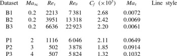
Table 1 reports the main properties of the turbulent boundary layers that we have investigated. Flow cases B1–B3 (mainly carried out for validation purposes) correspond to subsonic flow conditions, at various friction Reynolds numbers (
 $\mathit{Re}_{{\it\tau}}$
), whereas flow cases P1–P3 correspond to supersonic flow conditions at relatively low
 $\mathit{Re}_{{\it\tau}}$
, at various friction Mach numbers (
 $\mathit{Ma}_{{\it\tau}}$
). The free-stream values are denoted with an
 $\infty$
subscript. The mean velocity profiles and the associated eddy viscosity for flow cases B1–B3 have been obtained using the model proposed by Monkewitz et al. (Reference Monkewitz, Chauhan and Nagib2007), whereas for flow cases P1–P3 we have used the DNS database of Pirozzoli & Bernardini (Reference Pirozzoli and Bernardini2011).
Main properties of the investigated turbulent boundary layers:
 $C_{f}=2{\it\tau}_{w}/({\it\rho}_{\infty }U_{\infty }^{2})$
,
 $\mathit{Ma}_{{\it\tau}}=u_{{\it\tau}}/({\it\gamma}R\widetilde{T}_{w})^{1/2}$
,
 $\mathit{Re}_{{\it\tau}}=\overline{{\it\rho}}_{w}u_{{\it\tau}}{\it\delta}/\overline{{\it\mu}}_{w}={\it\delta}/{\it\delta}_{v}$
,
 ${\it\delta}$
is the 99 % boundary layer thickness,
 $\mathit{Re}_{{\it\theta}}={\it\rho}_{\infty }U_{\infty }{\it\theta}/{\it\mu}_{\infty }$
and
 ${\it\theta}$
is the momentum thickness.

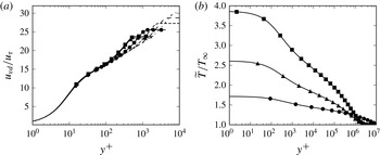
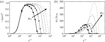
In figure 1 we show the mean streamwise velocity and temperature for the various flow cases, and in figure 2 we show the corresponding turbulent shear stress and turbulent viscosity profiles. It should be noted that the Van Driest transformation (Van Driest Reference Van Driest1951) is applied to the mean velocity,
 $u_{vd}=\int _{0}^{u}(\overline{{\it\rho}}/\overline{{\it\rho}}_{w})^{1/2}\,\text{d}\overline{u}$
, and the turbulent shear stress is scaled with the density ratio, as customary in the compressible formalism. The data are given in wall units (denoted with a
 $+$
superscript) based on the friction velocity
 $u_{{\it\tau}}=({\it\tau}_{w}/\overline{{\it\rho}}_{w})^{1/2}$
, and the wall viscous length scale
 ${\it\delta}_{v}={\it\nu}_{w}/u_{{\it\tau}}$
.
(a) The Van Driest-transformed mean velocity and (b) the Favre-averaged mean temperature. For the subsonic cases the mean velocity profiles proposed by Monkewitz et al. (Reference Monkewitz, Chauhan and Nagib2007) are shown. Refer to table 1 for nomenclature.

(a) Turbulent shear stress and (b) eddy viscosity. The asterisk denotes density-scaled quantities, reported in wall units. For the subsonic cases the fits given by Monkewitz et al. (Reference Monkewitz, Chauhan and Nagib2007) are shown. Refer to table 1 for nomenclature.

2.3. Analysis of transient growth
Significant experimental effort has been devoted to determining the organized motion driven by a harmonic forcing. For instance, to extract the organized structure of the flow in the near wake of a circular cylinder, Cantwell & Coles (Reference Cantwell and Coles1983) used an ensemble averaging process carried out on subpopulations, each one being associated with a particular phase interval (i.e. a phase average). In our approach, the organized motion is assumed to be driven by an initial condition. The coherent part of the motion can thus be investigated with an optimal transient growth analysis.
Let
 $\boldsymbol{q}=({\it\rho}^{\prime ,\ell },u^{\prime \prime ,\ell },v^{\prime \prime ,\ell },w^{\prime \prime ,\ell },T^{\prime \prime ,\ell })$
be the unknown vector representing the coherent part of the motion. Next, (i) we assume that the mean flow is homogeneous in the streamwise and spanwise directions
 $(\overline{{\it\rho}}(y),\widetilde{u}(y),0,0,\widetilde{T}(y))$
, and (ii) we introduce a Fourier decomposition for
 $\boldsymbol{q}$
:
 $$\begin{eqnarray}\boldsymbol{q}(x,y,z,t)=\boldsymbol{q}^{\prime }(y,t)\text{e}^{\text{i}({\it\alpha}x+{\it\beta}z)}+\text{c.c.}\end{eqnarray}$$
Here
 $\boldsymbol{q}^{\prime }$
is the mode amplitude (in the following, referred to as the Fourier mode or simply as the mode), and
 ${\it\alpha}$
and
 ${\it\beta}$
are, respectively, the wavenumbers in the
 $x$
and
 $z$
directions (
 ${\it\alpha}=2{\rm\pi}/{\it\lambda}_{x}$
,
 ${\it\beta}=2{\rm\pi}/{\it\lambda}_{z}$
), and c.c. denotes the complex conjugate. Substituting (2.15) into the linearized equations (2.9)–(2.11), the resulting dynamical system for
 $\boldsymbol{q}^{\prime }$
is
 $$\begin{eqnarray}\frac{\partial \boldsymbol{q}^{\prime }}{\partial t}=\mathscr{L}\boldsymbol{q}^{\prime },\end{eqnarray}$$
whose derivation is fully reported in appendix A.
Introducing the ratio of the total energy associated with
 $\boldsymbol{q}^{\prime }$
(including the kinetic energy as well as the internal energy) to the total energy at the initial time, the optimal temporal energy growth over all possible
 $\boldsymbol{q}_{(t=0)}^{\prime }$
is defined as
 $$\begin{eqnarray}G({\it\alpha},{\it\beta},t)=\text{sup}_{\boldsymbol{q}_{(t=0)}^{\prime }}\frac{\Vert \boldsymbol{q}^{\prime }\Vert }{\Vert {\boldsymbol{q}^{\prime }}_{(t=0)}\Vert }.\end{eqnarray}$$
Here the norm
 $\Vert (\cdot )\Vert$
is based on the inner product defined by Chu (Reference Chu1965) and Hanifi, Schmid & Henningson (Reference Hanifi, Schmid and Henningson1996),
 $$\begin{eqnarray}(\boldsymbol{q}_{k}^{\prime },\boldsymbol{q}_{l}^{\prime })=\int _{0}^{L_{y}}\boldsymbol{q}_{k}^{\prime h}\,\unicode[STIX]{x1D63F}\,\boldsymbol{q}_{l}^{\prime }\,\text{d}y,\end{eqnarray}$$
where
 $(\cdot )^{h}$
denotes the transconjugate,
 $L_{y}$
is the upper boundary location and
 $\unicode[STIX]{x1D63F}$
is the diagonal matrix
 $(\overline{T}/[\overline{{\it\rho}}{\it\gamma}M_{\infty }^{2}],~\overline{{\it\rho}},~\overline{{\it\rho}},~\overline{{\it\rho}},~\overline{{\it\rho}}/[{\it\gamma}({\it\gamma}-1)\overline{T}M_{\infty }^{2}])$
.
In the analysis that follows, we consider the supremum of
 $G$
over all possible
 $t$
for a given wavenumber pair
 $({\it\alpha},{\it\beta})$
,
 $$\begin{eqnarray}G_{max}({\it\alpha},{\it\beta})=\text{sup}_{t}\,G({\it\alpha},{\it\beta},t),\end{eqnarray}$$
and the supremum of
 $G_{max}$
over all possible
 $({\it\alpha},{\it\beta})$
,
 $$\begin{eqnarray}G_{opt}=\text{sup}_{{\it\alpha},{\it\beta}}\,G_{max}({\it\alpha},{\it\beta}).\end{eqnarray}$$
Modes attaining maximum transient amplification
 $G_{max}$
for a given
 $({\it\alpha},{\it\beta})$
pair will hereafter be referred to as optimal modes, and modes attaining
 $G_{opt}$
will be referred to as absolute optimal modes. We also define
 $t_{max}$
and
 $t_{opt}$
as the times at which a given mode attains
 $G_{max}$
and
 $G_{opt}$
, respectively.
In the laminar regime, these quantities are usually computed through singular-value decomposition (SVD) of the operator
 $\text{e}^{\mathscr{L}t}$
(Schmid & Henningson Reference Schmid and Henningson2001). This approach is here extended to the turbulent case to solve the dynamical system (2.16). The initial optimal coherent mode is taken as the right singular vector associated with the largest singular value of
 $\text{e}^{\mathscr{L}t}$
. The dynamical system (2.16) is discretized by using a spectral collocation method along the normal direction. In order not to impose boundary conditions on the density at the wall and at the far field, we use a staggered mesh (as usually done in the incompressible case), whereby a Gauss–Lobatto grid is employed for the velocity and the temperature components of the modes, whereas a Gauss grid is used for the density component (Malik Reference Malik1990). The velocity and the temperature are set to zero at the wall, and assumed to vanish at the upper boundary. Similar boundary conditions are used for laminar adiabatic supersonic boundary layers by Hanifi et al. (Reference Hanifi, Schmid and Henningson1996) and Malik (Reference Malik1990) for both a transient and an asymptotic stability analysis. The SVD of the discrete exponential operator is based on a discrete adjoint operator obtained with a weighted matrix derived from spectral integration (Hanifi et al.
Reference Hanifi, Schmid and Henningson1996). Finally, the matrix exponentials are computed using the EXPOKIT library (Sidje Reference Sidje1998). A grid sensitivity analysis has been carried out, but for the sake of conciseness we only present the results obtained with the finest grid having 500 collocation points in the wall-normal direction.
The mean flow and the turbulent viscosity are obtained by interpolation of DNS statistics (Bernardini & Pirozzoli Reference Bernardini and Pirozzoli2011b ; Pirozzoli & Bernardini Reference Pirozzoli and Bernardini2011), using a cubic spline. The optimal energy growth associated with the dynamical system (2.16) has been computed for a wide range of streamwise and spanwise wavenumbers. The code has been validated for the linear transient growth of a laminar supersonic adiabatic boundary layer, obtaining favourable comparison with the results of Hanifi et al. (Reference Hanifi, Schmid and Henningson1996) (see appendix C). The code has also been validated for a turbulent subsonic boundary layer against the incompressible results of Cossu et al. (Reference Cossu, Pujals and Depardon2009) (the results will be shown later on).
3. Optimal transient growth
3.1. Optimal energy gain
The main goal here is to understand the influence of compressibility and mode orientation on the optimal energy growth, by considering several wavevectors
 $({\it\alpha},{\it\beta})$
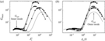
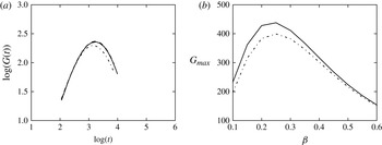
. In figure 3 we show the maximum total energy amplification (attained at the optimal time) of infinitely long structures (
 ${\it\alpha}=0$
) as a function of the spanwise wavelength, in inner (figure 3
a) and outer (figure 3
b) units. We find that
 $G_{max}$
exhibits two peaks, associated with maximum amplification in the inner and the outer layer, as also observed in turbulent incompressible boundary layers (Cossu et al.
Reference Cossu, Pujals and Depardon2009) and in channels (del Alamo & Jiménez Reference del Alamo and Jiménez2006; Pujals et al.
Reference Pujals, Garci-Villalba, Cossu and Depardon2009). The inner peak of
 $G_{max}$
scales in inner units, and corresponds to a spanwise wavelength
 ${\it\lambda}_{z}^{+}\approx 81$
(
 ${\it\lambda}_{z}^{+}={\it\lambda}_{z}/{\it\delta}_{v}$
). The outer peak scales in outer units, and corresponds to a spanwise wavelength
 ${\it\lambda}_{z}\approx 8.5{\it\delta}$
, where
 ${\it\delta}$
is the 99 % boundary layer thickness. These values are consistent with those obtained by Cossu et al. (Reference Cossu, Pujals and Depardon2009) for incompressible boundary layers. The distance from the wall (
 $y_{max}$
) at which the maximum gain in total energy occurs also confirms the occurrence of the double scaling, as shown in figure 4, where it is reported as a function of the spanwise wavelength. In particular, the inner peak occurs at
 $y_{max}^{+}\approx 10$
, whereas the outer peak is found at
 $y_{max}/{\it\delta}\approx 0.8{\it\delta}$
. Overall, it appears that scale separation is driven by variation of
 $\mathit{Re}_{{\it\tau}}$
, rather than by variation of the Mach number. In the intermediate range of spanwise wavenumbers, we also observe a region where the maximum growth is nearly constant. This property has also been observed in optimal transient growth calculations of channel flows and boundary layers (del Alamo & Jiménez Reference del Alamo and Jiménez2006; Cossu et al.
Reference Cossu, Pujals and Depardon2009; Pujals et al.
Reference Pujals, Garci-Villalba, Cossu and Depardon2009). Recently, Hwang & Cossu (Reference Hwang and Cossu2010a
) have shown that this region is associated with the amplification of log-layer structures.
Maximum total energy amplification (
 $G_{max}$
) as a function of the spanwise wavelength in (a) inner and (b) outer units, for infinitely elongated structures (
 ${\it\alpha}=0$
). Refer to table 1 for nomenclature.

Wall-normal position (
 $y_{max}$
) of the peak of
 $G_{max}$
as a function of the spanwise wavelength in (a)inner and (b) outer units, for infinitely elongated structures (
 ${\it\alpha}=0$
). Refer to table 1 for nomenclature.

3.2. Inner-layer optimal modes
We now focus on the near-wall peak of
 $G_{max}$
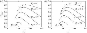
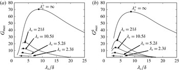
, which is shown in figure 5 as a function of the spanwise wavelength for several values of the streamwise wavelength. As noted above, the absolute optimal growth is found to be associated with infinitely elongated coherent structures having a spanwise size of approximately 80 wall units. Figure 5 further suggests that the most amplified inner-layer modes have proportional values of
 ${\it\lambda}_{x}$
and
 ${\it\lambda}_{z}$
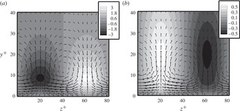
, and hence the longer optimal modes are also wider. In figure 6 we show the velocity and temperature maps corresponding to the absolute optimal mode in the cross-stream plane. The arrows in the figure represent the velocity vectors at the initial time. As in the incompressible regime, a peculiar lift-up effect (Landahl Reference Landahl1980) is observed, which is seen to be responsible for the optimal growth. Figure 6 also shows that the temperature pattern is strictly related to the velocity pattern, and positive (respectively, negative) temperature fluctuations strongly correlate with low-speed (respectively, high-speed) streaks. This is in agreement with the well-known tendency of velocity and temperature fluctuations to be negatively correlated in turbulent supersonic boundary layers Pirozzoli & Bernardini (Reference Pirozzoli and Bernardini2011). The temperature here seems to have a relatively passive role, while the streamwise vortices at the initial time act to redistribute momentum and temperature through sweeps and ejections.
Inner-layer modes: optimal gain as a function of the spanwise wavelength for different streamwise wavelengths, for (a) flow case B1 and (b) flow case P1. The asterisks denote the value of
 $\sup _{{\it\beta}}G_{max}({\it\alpha},{\it\beta})$
.

Inner-layer modes, P1 flow case: contours of (a) streamwise velocity and (b) temperature in the cross-stream plane, with superimposed cross-stream velocity vectors, for the absolute optimal mode (
 ${\it\alpha}=0$
,
 ${\it\lambda}_{z}^{+}=81$
).

The maps of
 $G_{max}$
and
 $t_{max}$
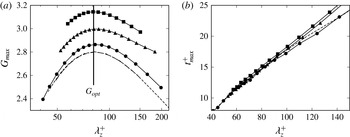
for two-dimensional optimal modes are shown in figure 7 for all the flow cases. The maximum transient amplification (figure 7
a) is found to be more affected by Mach number variation rather than by Reynolds number variation, and
 $G_{opt}$
is found to vary from 2.8 at
 $\mathit{Ma}_{\infty }=0.2$
to 3.2 at
 $\mathit{Ma}_{\infty }=4$
. However, the spanwise length scale of the optimal mode is weakly affected by compressibility, and
 ${\it\lambda}_{z}^{+}\approx 81.5$
in all cases, as also found in the incompressible case (Cossu et al.
Reference Cossu, Pujals and Depardon2009). It is worth pointing out that the length scale recovered with the present linear model is also consistent with the size of the streaks found in DNS of supersonic turbulent boundary layers (Pirozzoli & Bernardini Reference Pirozzoli and Bernardini2013). Figure 7(b) shows that the typical time scale of the structures attaining the maximum amplification is nearly independent of the Mach number, and it varies linearly with the spanwise wavelength.
Inner-layer modes: (a) maximum energy gain and (b) corresponding time
 $t_{max}$
as functions of the spanwise wavelength for
 ${\it\alpha}=0$
. Refer to table 1 for nomenclature.

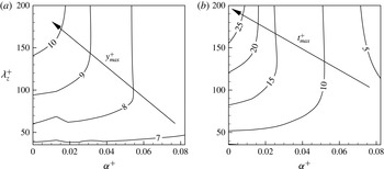
Figure 8(a) shows iso-lines of the wall distance at which
 $G_{max}$
is attained in the P1 flow case, and figure 8(b) shows the corresponding optimal times
 $t_{max}$
as a function of the streamwise and spanwise wavenumbers. It is found that both
 $y_{max}$
and
 $t_{max}$
increase as
 ${\it\alpha}$
and
 ${\it\beta}$
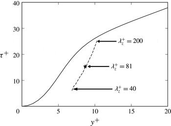
decrease. We recall that in wall-bounded turbulent shear flows coherent structures are disrupted on a time scale of the order of the eddy turnover time
 ${\it\tau}=k/{\it\varepsilon}$
, where
 $k=\overline{{\it\rho}}\widetilde{u_{k}^{\prime \prime }u_{k}^{\prime \prime }}/2$
is the turbulent kinetic energy and
 ${\it\varepsilon}=\overline{{\it\mu}(\partial u_{i}^{\prime }/\partial x_{j})(\partial u_{i}^{\prime }/\partial x_{j})}$
is its dissipation rate (Lee, Kim & Moin Reference Lee, Kim and Moin1990; Butler & Farrel Reference Butler and Farrel1992). Hence, only coherent modes having temporal scale less than the eddy turnover time are physically acceptable solutions. In figure 9 we then report the distribution of
 ${\it\tau}$
as a function of the wall distance, together with the optimal time of infinitely elongated modes (
 $t_{max}(0,{\it\beta})$
), which, based on the previous considerations, have the longer lifetimes, at the corresponding distances (
 $y_{max}(0,{\it\beta})$
). The eddy turnover time is estimated from the DNS database of Pirozzoli & Bernardini (Reference Pirozzoli and Bernardini2011). Figure 9 shows that
 $t_{max}$
does not exceed the eddy turnover time for the most amplified optimal modes that we have analysed. This leads to the conclusion that the coherent modes retrieved through the transient growth analysis are physically relevant.
Inner-layer modes, flow case P1: maps of (a) wall distance and (b) time
 $t_{max}$
at which amplification is maximum.

Inner-layer modes: eddy turnover time as a function of wall distance for flow case P1. The dashed line denotes the optimal time of infinitely elongated modes (
 $t_{max}(0,{\it\beta})$
) at the corresponding distances (
 $y_{max}(0,{\it\beta})$
), for
 ${\it\lambda}_{z}^{+}$
from 40 to 200. The asterisk denotes the absolute optimal mode.

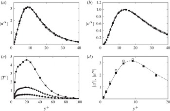
The contributions to the growth of the absolute optimal mode are separately shown in figure 10, at the initial time (panel (b)) and at the optimal time (panels (a), (c) and (d)), where for the supersonic cases the density-scaled velocity components (3.1) are reported, namely
 $$\begin{eqnarray}{u^{\prime }}^{\ast }=\sqrt{\frac{\overline{{\it\rho}}}{\overline{{\it\rho}}_{w}}}u^{\prime },\quad {v^{\prime }}^{\ast }=\sqrt{\frac{\overline{{\it\rho}}}{\overline{{\it\rho}}_{w}}}v^{\prime }.\end{eqnarray}$$
In figure 10(d) the unscaled velocity is shown for comparison, limited to flow case P3. In agreement with Morkovin’s hypothesis, figure 10(d) shows the similarity of the kinematic components of the optimal mode, and better collapse is achieved through density scaling. On the other hand, temperature exhibits a peak that increases with the Mach number. In this respect we recall that, based on the chosen energy norm given in (2.18),
 $G$
incorporates the contribution of both the kinetic energy and the internal energy. Hence, temperature growth is the main cause for the overall increase of the optimal gain with the Mach number observed in figure 7.
Inner-layer modes, amplitude of the components of the absolute optimal modes, scaled with respect to their initial value: (a)
 ${u^{\prime }}^{\ast }$
at
 $t_{opt}$
; (b)
 ${v^{\prime }}^{\ast }$
at the initial time; (c)
 $T^{\prime }$
at
 $t_{opt}$
; and (d)
 ${u^{\prime }}^{\ast }$
at
 $t_{opt}$
, limited to flow case P3 (open symbols indicate that density scaling is not used).

To quantify the kinetic energy contribution to the energy gain, we introduce the following metric:
 $$\begin{eqnarray}G_{max}^{k}({\it\alpha},{\it\beta})=\frac{\displaystyle \int _{0}^{L_{y}}\overline{{\it\rho}}\,\boldsymbol{u}^{\prime h}\boldsymbol{u}^{\prime }\,\text{d}y_{(t=t_{max})}}{\displaystyle \int _{0}^{L_{y}}\overline{{\it\rho}}\,\boldsymbol{u}^{\prime h}\boldsymbol{u}^{\prime }\,\text{d}y_{(t=0)}},\end{eqnarray}$$
where
 $\boldsymbol{u}^{\prime }=(u^{\prime },v^{\prime },w^{\prime })$
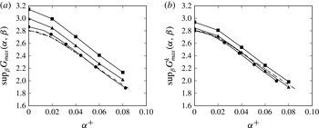
. The distribution of
 $\sup _{{\it\beta}}G_{max}({\it\alpha},{\it\beta})$
and its kinetic counterpart is reported in figure 11 as a function of the streamwise wavenumber. As one would expect, we note that kinetic energy contributes most to
 $G_{max}$
, and its increase with respect to the incompressible case is mainly associated with the amplification of the internal energy. On the other hand, the kinetic energy contribution is weakly affected by the Mach number, and the curves nearly collapse for Mach number up to 3.
Inner-layer modes: distributions of (a)
 $\sup _{{\it\beta}}G_{max}({\it\alpha},{\it\beta})$
and (b) kinetic energy contribution as a function of the streamwise wavenumber. Refer to table 1 for nomenclature.

To further elucidate the mechanisms of energy transfer between the kinetic and the internal energy, we have analysed the corresponding energy budgets for the absolute optimal mode. Let
 $\mathscr{E}$
be the integrated total energy in the wall-normal direction
 $$\begin{eqnarray}\mathscr{E}=\mathscr{E}^{k}+\mathscr{E}^{in},\end{eqnarray}$$
where
 $\mathscr{E}^{k}$
and
 $\mathscr{E}^{in}$
are the kinetic energy and the internal energy, respectively. The evolution of
 $\mathscr{E}$
is described by (Malik, Meheboob & Dey Reference Malik, Meheboob and Dey2006)
 $$\begin{eqnarray}\frac{\text{d}\mathscr{E}}{\text{d}t}=\int _{0}^{L_{y}}\boldsymbol{q}^{\prime h}\unicode[STIX]{x1D63F}\mathscr{L}\boldsymbol{q}^{\prime }\,\text{d}y+\text{c.c.},\end{eqnarray}$$
where the energy is normalized by the total energy associated with the initial optimal coherent mode. The budget of the kinetic energy is written in the form
 $$\begin{eqnarray}\frac{\text{d}\mathscr{E}^{k}}{\text{d}t}=\mathscr{P}^{k}-\mathscr{D}_{v}^{k}-\mathscr{D}_{t}^{k},\end{eqnarray}$$
where
 $\mathscr{P}^{k},\mathscr{D}_{v}^{k}$
and
 $\mathscr{D}_{t}^{k}$
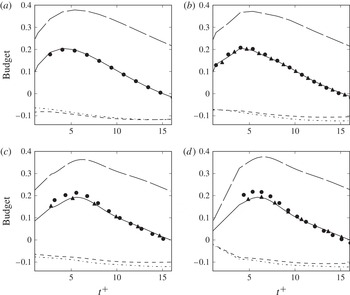
represent, respectively, the production due to mean shear, the dissipation associated with molecular viscosity and the turbulent dissipation at the small scales (see appendix B for their definition). The contributions to (3.5) are shown in figure 12. The evolution of the total energy is found to be mainly driven by its kinetic part, and in particular by production due to mean shear,
 $\mathscr{P}^{k}$
. Furthermore, the time rate of change of the energy of the optimal inner mode attains its maximum on a time scale corresponding to the peak production. One may note that the optimal gain (for which
 $\text{d}\mathscr{E}/\text{d}t=0$
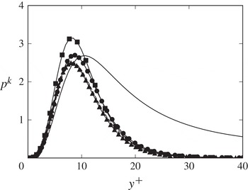
) corresponds to an equilibrium state where dissipation is balanced by production, and as previously noted this mechanism is weakly affected by the Mach number. We also note that the dissipation caused by molecular diffusion and caused by turbulent coherent motions are of the same order of magnitude. It is then evident that the latter contribution cannot be neglected when carrying out the linear stability analysis of a turbulent mean flow, thus corroborating the statements of del Alamo & Jiménez (Reference del Alamo and Jiménez2006) and Cossu et al. (Reference Cossu, Pujals and Depardon2009) for the incompressible case. Figure 13 shows the wall-normal profile of the local kinetic energy production (
 $p^{k}(y)=-\overline{{\it\rho}}\,u^{\prime h}v^{\prime }\,\text{d}\overline{u}/\text{d}y$
), at the time at which
 $\mathscr{P}^{k}$
attains its maximum. It is found that
 $p^{k}$
attains a peak at
 $y^{+}\approx 10$
, which well matches the innermost layer distribution found in DNS (Pirozzoli & Bernardini Reference Pirozzoli and Bernardini2011), upon suitable rescaling, thus supporting the important role played by coherent motions in the establishment of the turbulence kinetic energy peak.
Inner-layer modes: energy budget of the optimal mode for (a) flow case B1, (b) flow case P1, (c) flow case P2 and (d) flow case P3. Nomenclature: solid,
 $\text{d}\mathscr{E}_{k}/\text{d}t$
; long dashed,
 $\mathscr{P}^{k}$
; short dashed,
 $\mathscr{D}_{v}^{k}$
; dot-dashed,
 $\mathscr{D}_{t}^{k}$
; circles,
 $\text{d}\mathscr{E}/\text{d}t$
; triangles,
 $\mathscr{P}^{k}+\mathscr{D}_{v}^{k}+\mathscr{D}_{t}^{k}$
(see (3.5)).

Inner-layer modes, distribution of the local kinetic energy production,
 $p^{k}(y)$
, normalized by its initial value, at the time at which
 $\mathscr{P}^{k}$
attains its maximum. The DNS data of Pirozzoli & Bernardini (Reference Pirozzoli and Bernardini2011) are shown with a solid line, in arbitrary units. Refer to table 1 for nomenclature.

Iso-contour lines of the streamwise (
 ${\it\omega}_{x}$
), wall-normal (
 ${\it\omega}_{y}$
) and spanwise (
 ${\it\omega}_{z}$
) vorticity components of the absolute optimal mode and an oblique optimal mode
 $\sup _{{\it\beta}}G_{max}(0.08/{\it\delta}_{v},{\it\beta})$
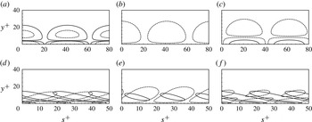
are shown in figure 14, in a plane orthogonal to the associated wavevector. Vortical structures associated with the absolute optimal mode (figure 14
a–c) are two-dimensional, and are stretched in the streamwise direction, undergoing a lift-up mechanism whereby vorticity is transferred from the streamwise to the wall-normal direction. Vortical structures associated with a three-dimensional optimal mode are shown in figure 14(d–f) for
 ${\it\lambda}_{x}^{+}=78$
,
 ${\it\lambda}_{z}^{+}=55$
, which corresponds (see figure 5) to
 $\sup _{{\it\beta}}G_{max}(0.08/{\it\delta}_{v},{\it\beta})$
. This particular three-dimensional mode (similarly to many others, not shown) is dominated by tilting in the shear direction, according to the Orr mechanism. The linear model thus incorporates the two main mechanisms associated with the intensification of vortical structures in turbulent shear flows. Similar observations also hold at higher Mach number (the figures are not shown for brevity).
Inner-layer modes, flow case P1: vorticity contours in planes normal to the wavevector for (a–c) the absolute optimal (two-dimensional) mode and (d–f) the optimal three-dimensional mode having
 ${\it\lambda}_{x}^{+}=78$
,
 ${\it\lambda}_{z}^{+}=55$
. Axis label
 $s$
denotes the wall-parallel coordinate normal to the wavevector. The streamwise, wall-normal and spanwise vorticity components are shown in panels (a,d), (b,e) and (c,f), respectively. Solid lines correspond to the initial time, and dashed lines to the optimal time.

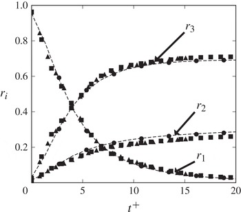
To characterize the influence of compressibility on the lift-up mechanism, the time evolution of the integrated enstrophy ratios (Guegan, Huerre & Schmid Reference Guegan, Huerre and Schmid2007; Alizard, Robinet & Guiho Reference Alizard, Robinet and Guiho2013),
 $r_{\ell }={\it\Omega}_{\ell }/\sum _{i}{\it\Omega}_{i}$
, where
 ${\it\Omega}_{i}=\int _{\mathscr{D}}{\it\omega}_{i}^{2}(t)\,\text{d}D$
, are analysed for the absolute optimal mode. Figure 15 confirms that the initial optimal vorticity field is mainly oriented in the streamwise direction, whereas the wall-normal and the spanwise vorticity components are amplified under the action of the mean shear. Figure 15 also shows the collapse of all the curves, thus confirming that the vorticity transfer mechanism is weakly affected by the Mach number.
Inner-layer modes: time evolution of the enstrophy ratios for the absolute optimal mode. Refer to table 1 for nomenclature.

3.3. Outer-layer optimal modes
To characterize the properties of the most amplified outer-layer modes, we have also computed the singular vectors associated with the maximum kinetic energy amplification
 $G_{max}^{k}({\it\alpha},{\it\beta})$
, for a wide range of streamwise and spanwise wavelengths. Note that the kinetic energy contribution is only retained to compare the supersonic cases with the subsonic ones. In figure 16 we show the kinetic energy contribution to the maximum energy gain as a function of the spanwise wavelength for different streamwise wavelengths, and mark with asterisks the values of
 $\sup _{{\it\beta}}G_{max}^{k}({\it\alpha},{\it\beta})$
. Figure 16 indicates that the most amplified outer-layer structures correspond to a particular combination of
 $({\it\lambda}_{x},{\it\lambda}_{z})$
that weakly depends on the Mach number. As for the inner-layer modes, it is found that the absolute optimal modes correspond to infinitely elongated streamwise structures, whose typical spanwise size is approximately
 $8{\it\delta}$
.
Outer-layer modes: optimal gain
 $G_{max}^{k}$
as a function of the spanwise wavelength for different streamwise wavelengths for (a) flow case B1 and (b) flow case P1. The asterisks denote the positions of
 $\sup _{{\it\beta}}G_{max}^{k}({\it\alpha},{\it\beta})$
.

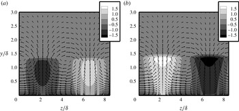
In figure 17 we show the velocity and temperature maps corresponding to the outer optimal mode in the cross-stream plane, for flow case P1. The arrows in the figure represent the velocity vectors at the initial time. As in the incompressible regime, the optimal initial coherent structures are found to be associated with streamwise vortices that lead to streamwise streaks. Strong negative correlation of
 $u^{\prime \prime ,\ell }$
and
 $T^{\prime \prime ,\ell }$
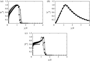
is found, as in the inner layer. Similar results, not shown, are also obtained for the P2 and P3 flow cases. The contributions to the growth of the absolute optimal mode are separately shown in figure 18, at the initial time (figure 18
b) and at the optimal time (figure 18
a,c), where density-scaled velocity components are reported for the supersonic cases. As in the inner layer, and in agreement with Morkovin’s hypothesis, similarity still holds for the kinematic components of the optimal outer mode, and good collapse is achieved through density scaling.
Outer-layer modes, P1 flow case: contours of (a) streamwise velocity and (b) temperature in the cross-stream plane, with superimposed cross-stream velocity vectors, for the absolute optimal mode (
 ${\it\alpha}=0$
,
 ${\it\lambda}_{z}=8.5{\it\delta}$
).

Outer-layer modes, amplitude of the components of the absolute optimal mode, scaled with respect to their initial value: (a)
 ${u^{\prime }}^{\ast }$
at
 $t_{opt}$
; (b)
 ${v^{\prime }}^{\ast }$
at the initial time; and (c)
 $T^{\prime }$
at
 $t_{opt}$
.

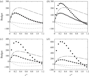
Regarding the energy budgets (reported in figure 19), we find that, on a short time scale (
 $t/t_{opt}\approx 0.2{-}0.4$
), the coherent dynamics is strongly affected by the internal energy. When the energy attains its optimal gain (
 $t/t_{opt}=1$
), an equilibrium state is reached, and the production of kinetic energy balances its dissipation, as also observed for the inner peak. When this state is reached, the role played by the internal energy becomes marginal. Turbulent dissipation is found to be much larger in this case than the molecular one, as expected in the outer layer.
Outer-layer modes: energy budget for the optimal mode for (a) flow case B1, (b) flow case P1, (c) flow case P2 and (d) flow case P3. Nomenclature: solid,
 $\text{d}\mathscr{E}_{k}/\text{d}t$
; long dashed,
 $\mathscr{P}^{k}$
; short dashed,
 $\mathscr{D}_{v}^{k}$
; dot-dashed,
 $\mathscr{D}_{t}^{k}$
; circles,
 $\text{d}\mathscr{E}/\text{d}t$
; triangles,
 $\mathscr{P}^{k}+\mathscr{D}_{v}^{k}+\mathscr{D}_{t}^{k}$
(see (3.5)).

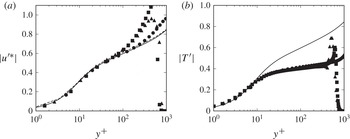
To verify the physical relevance of the optimal outer coherent modes on the inner-layer dynamics, in figure 20 we show their amplitude as a function of the inner-scaled wall distance. As also noted by Pujals et al. (Reference Pujals, Garci-Villalba, Cossu and Depardon2009) for incompressible channel flows, we find collapse of the curves up to
 $y^{+}\approx 100$
for all the flow cases. Furthermore, the velocity and the temperature amplitudes vary linearly up to
 $y^{+}\approx 10$
, and the amplitude of the mode is found to be proportional of the mean velocity. A similar signature was observed by Cossu et al. (Reference Cossu, Pujals and Depardon2009).
Outer-layer modes: normalized amplitude of (a) streamwise velocity and (b) temperature for the absolute optimal mode based on the reference subsonic case B1. The solid line represents the mean streamwise velocity. Refer to table 1 for nomenclature.

Regarding the structural properties of outer-layer eddies, DNS and experiments (Ganapathisubramani, Clemens & Dolling Reference Ganapathisubramani, Clemens and Dolling2006; Pirozzoli & Bernardini Reference Pirozzoli and Bernardini2011) show that the organized structures have a rather universal behaviour, in that their characteristic scales and orientations are weakly affected by compressibility. In particular, in agreement with low-speed turbulent boundary layers (Tomkins & Adrian Reference Tomkins and Adrian2003; Marusic & Heuer Reference Marusic and Heuer2007), DNS data (Pirozzoli & Bernardini Reference Pirozzoli and Bernardini2011) at
 $\mathit{Ma}_{\infty }=2$
show that the typical size of outer-layer eddies is approximately
 $1{\it\delta}$
in the streamwise direction, and approximately
 $0.5{\it\delta}$
in the spanwise direction, and their typical streamwise inclination angle is
 ${\approx}12^{\circ }{-}14^{\circ }$
.
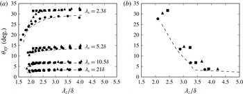
To quantitatively characterize the orientation of outer-layer modes educed from transient growth analysis, we consider their projected angle in the
 $x{-}y$
plane, estimated from the wall-normal position (
 $y_{max}$
) where the streamwise velocity is maximum at the optimal time, and half the streamwise wavelength,
 ${\it\theta}_{xy}=\text{tan}^{-1}(2y_{max}/{\it\lambda}_{x})$
. Figure 21 shows
 ${\it\theta}_{xy}$
as a function of the spanwise wavelength, for various streamwise wavelengths. In the incompressible case the inclination angle is not affected by the Reynolds number, and collapse of flow cases B1–B3 is observed in a wide range of wavenumbers. The results of the P1 flow case are also in excellent agreement with the subsonic one, whereas deviations are observed for flow cases P2 and P3.
Outer-layer modes: (a) inclination angle of modes attaining
 $G_{max}^{k}$
, shown as a function of the spanwise wavelength for various streamwise wavelengths; (b) inclination angles as a function of
 ${\it\lambda}_{z}$
for modes attaining
 $\sup _{{\it\beta}}G_{max}^{k}({\it\alpha},{\it\beta})$
. All the subsonic cases are collapsing. Refer to table 1 for nomenclature.

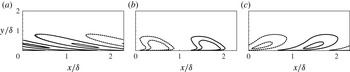
Outer-layer modes, flow case P1: streamwise velocity contours for the mode associated with
 ${\it\lambda}_{x}=2.3{\it\delta}$
and
 ${\it\lambda}_{z}=1.5{\it\delta}$
(having
 ${\it\theta}_{xy}=15^{\circ }$
), at (a)
 $t/t_{max}=0$
, (b)
 $t/t_{max}=0.27$
and (c)
 $t/t_{max}=1$
. Solid lines represent positive values and dashed lines negative values.

Figure 21(a,b) further shows that the inclination angle is a decreasing functions of
 ${\it\lambda}_{x}$
and
 ${\it\lambda}_{z}$
. Hence, larger structures have a tendency to lean towards the wall, whereas smaller structures have a tendency to be tilted with respect to it. As the Mach number increases, the inclination angle increases, and the location where the velocity is maximum shifts away from the wall, meaning that organized structures have greater tendency to be tilted and lifted up from the wall. These results are consistent with the DNS data of Duan et al. (Reference Duan, Beekman and Martin2011), who explored the effect of the Mach number on turbulent boundary layers up to
 $\mathit{Ma}_{\infty }=12$
. For flow case P1, we find that the coherent structures associated with
 $G_{max}^{k}(2{\rm\pi}/{\it\lambda}_{x},2{\rm\pi}/{\it\lambda}_{z})$
,
 ${\it\lambda}_{x}=2.3{\it\delta}$
and
 ${\it\lambda}_{z}=1.5{\it\delta}$
, have an inclination angle of
 ${\it\theta}_{xy}\approx 15^{\circ }$
. This particular optimal mode is then compatible with the DNS findings (Pirozzoli & Bernardini Reference Pirozzoli and Bernardini2011). The streamwise velocity maps for this mode are shown in figure 22 at various stages of its evolution, from
 $t=0$
to
 $t_{max}$
. Notably, the distance at which the velocity is maximum is less than for infinitely elongated streaks (see figure 18
a). This is consistent with the experiments of Ganapathisubramani et al. (Reference Ganapathisubramani, Clemens and Dolling2006), who observed an increasing trend of the streamwise length scale with the wall distance.
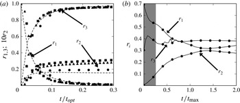
Outer-layer modes: time evolution of the enstrophy ratios for (a) the absolute optimal mode and (b) a three-dimensional mode having
 ${\it\lambda}_{x}=2.3{\it\delta}$
and
 ${\it\lambda}_{z}=1.5{\it\delta}$
(having
 ${\it\theta}_{xy}=15^{\circ }$
). The grey area in panel (b) represents the time necessary for the structure to reach the pattern shown in figure 22(b). Refer to table 1 for nomenclature.

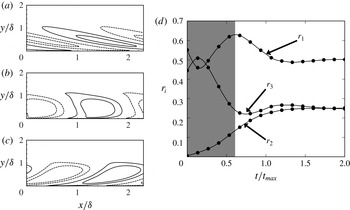
In figure 23 we show the time evolution of the enstrophy ratios for the absolute optimal outer-layer mode and for the three-dimensional ‘DNS-compatible’ mode, having
 ${\it\lambda}_{x}=2.3{\it\delta}$
and
 ${\it\lambda}_{z}=1.5{\it\delta}$
. Figure 23(a) shows that a similar vorticity transfer mechanism holds as in the inner layer. For the three-dimensional modes (see figure 23(b) for the P1 flow case), in a first stage (shaded in grey), the mode is reoriented along the shear direction under the action of the Orr mechanism. Then, the mode undergoes a lift-up mechanism, whereby streamwise vorticity is primarily reoriented to the wall-normal direction. Hence, the most relevant structures compatible with experiments and DNS appear to combine the effects of the Orr and of the lift-up mechanisms (Farrell & Ioannou Reference Farrell and Ioannou1993). In figure 24 we show the streamwise velocity contours at various times in panels (a–c) and the time evolution of the enstrophy ratios in panel (d) for the optimal three-dimensional mode reaching
 $\sup _{{\it\beta}}G_{max}^{k}(2{\rm\pi}/{\it\lambda}_{x},2{\rm\pi}/{\it\lambda}_{z})$
for
 ${\it\lambda}_{x}=2.3{\it\delta}$
. Figures 22 and 24 show that the optimal structure and the most compatible one exhibit a similar pattern. However, the optimal structure has an inclination angle that is nearly twice the value observed in experiments and in DNS, and experiences Orr/lift-up mechanisms on a longer time scale (figure 24
d). A similar behaviour is recovered at all Mach numbers.
Outer-layer modes, flow case P1: (a–c) streamwise velocity contours for the mode associated with
 ${\it\lambda}_{x}=2.3{\it\delta}$
and
 ${\it\lambda}_{z}=2{\it\delta}$
(having
 ${\it\theta}_{xy}=27^{\circ }$
), at (a)
 $t/t_{max}=0$
, (b)
 $t/t_{max}=0.67$
and (c)
 $t/t_{max}=1$
(solid lines represent positive values and dashed lines negative values); and (d) time evolution of the enstrophy ratios. The grey area in panel (d) represents the time necessary for the structure to reach the pattern shown in panel (b).

3.4. Log-layer optimal modes
The amplification curves in figure 3 showed the existence of a log-layer region between the inner- and outer-layer peaks, where the total energy gain attains a near plateau, and which is the subject of the present section. In the past a lot of interest has been devoted to the logarithmic part of the wall layer. According to the classical scenario (Townsend Reference Townsend1976), this region is populated by a host of self-similar attached eddies, whose size is proportional to the wall distance. One of the consequences of this assumption is that the variances of the wall-parallel velocity fluctuations should scale logarithmically with the wall distance. Townsend’s attached-eddy hypothesis has received support from the experiments of Tomkins & Adrian (Reference Tomkins and Adrian2003), who noted that the spanwise length scale of eddies in the log layer varies linearly with the wall distance, and logarithmic decay of the velocity variances has been recovered in a number of studies (see Marusic et al. (Reference Marusic, Monty, Hultmark and Smits2013) for an overview). The turbulence self-sustainment processes in the log layer were studied through filtered DNS in minimal boxes by Hwang & Cossu (Reference Hwang and Cossu2011). They found that the characteristic spanwise scales associated with the surviving motions follow a linear scaling with the wall distance. More recently, Moarref et al. (Reference Moarref, Sharma, Tropp and McKeon2013) confirmed the important role of linear processes in establishing a self-similar hierarchy of coherent eddies in the log layer. Their results further supported the hypothesis that linear amplification of optimal modes in the logarithmic layer leads to streaky motions, which may regenerate after bursting, and which exhibit a universal behaviour, when scaled by their spanwise extent. Modes belonging to the intermediate region are hereafter referred to as log-layer optimal modes.
In order to verify if supersonic boundary layers also exhibit geometrical similarity, we study the dependence of the log-layer optimal modes on the spanwise wavelength, limiting our analysis to infinitely elongated modes (
 ${\it\alpha}=0$
) that are the most amplified.
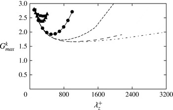
The kinetic energy amplification curves are shown in figure 25 as a function of the spanwise wavenumber, in a linear scale. As previously noticed in § 3.2, the
 $G_{max}^{k}$
data fall on a nearly universal curve close to the inner peak, and tend to form a plateau as the Reynolds number increases. Figure 25 also shows a slight shift of the minimum value for
 $G_{max}^{k}$
when increasing the Mach number from 3 to 4.
Maximum kinetic energy gain for infinitely elongated optimal modes (
 ${\it\alpha}=0$
) as a function of the spanwise wavelength. Refer to table 1 for nomenclature of lines.

To characterize the vertical size of the optimal log-layer modes, we define a typical length scale (
 ${\it\Lambda}_{y}$
) as the wall distance at which the cumulative modal kinetic energy is 80 % of the total, i.e.
 $$\begin{eqnarray}\int _{0}^{{\it\Lambda}_{y}}\overline{{\it\rho}}u^{2}\,\text{d}{\it\eta}=0.8\int _{0}^{\infty }\overline{{\it\rho}}u^{2}\,\text{d}{\it\eta},\end{eqnarray}$$
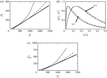
where all quantities are evaluated at the time at which kinetic energy is maximum. The relevance of this length scale for describing self-similarity of the log layer is first established by analysing the subsonic flow cases B1–B3. The results are summarized in figure 26, which in fact shows linear variation of
 ${\it\Lambda}_{y}$
on
 ${\it\lambda}_{z}$
, regardless of the Reynolds number. The corresponding optimal modes, shown in figure 26(b) as a function of the wall distance scaled by the spanwise wavelength, support geometrical similarity of the log-layer modes, in agreement with Townsend’s attached-eddy model (Townsend Reference Townsend1976). Finally, figure 26(c) indicates that the optimal time for these modes also varies linearly with
 ${\it\lambda}_{z}$
. This finding is consistent with the claim of del Alamo et al. (Reference del Alamo, Jiménez, Zandonade and Moser2006) that the lifetime of the log-layer eddies is proportional to their size. Finally, figure 26(a,c) shows that, for subsonic Mach numbers, modes larger than
 ${\it\lambda}_{z}\approx 0.43{\it\delta}$
(corresponding to
 ${\it\lambda}_{z}^{+}=950$
, 1700 and 2850 for B1, B2 and B3, respectively) deviate from the universal behaviour and they are mostly affected by the outer motion.
Subsonic log-layer optimal modes (for
 ${\it\alpha}=0$
). (a) Vertical length scale as a function of spanwise wavelength for flow case B1–B3. (b) Mode amplitudes as a function of wall distance scaled by spanwise wavelength: B1 (
 ${\it\lambda}_{z}^{+}=770$
), B2 (
 ${\it\lambda}_{z}^{+}=863$
) and B3 (
 ${\it\lambda}_{z}^{+}=893,1250,2084$
), where
 $u^{\prime }$
is taken at
 $t=t_{max}$
, and
 $v^{\prime }$
at
 $t=0$
. (c) Optimal time as a function of the spanwise wavelength. The solid lines indicate the linear fit of the data. Refer to table 1 for nomenclature.

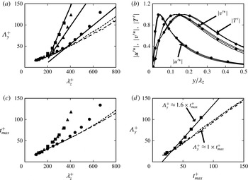
Similar data are shown in figure 27 for the supersonic flow cases. In fact, figure 27(a) confirms that the vertical length scale of the optimal modes scales linearly with the spanwise wavelength also in supersonic boundary layers. The modal velocity and temperature distributions, shown in figure 27(b), do exhibit geometrical similarity, thus suggesting that Townsend’s attached-eddy model also applies to supersonic boundary layers. The rescaled optimal modes also bear strong similarities with the buffer-layer modes, indicating that kinetic energy grows through a similar lift-up mechanism. The optimal time scale, shown in figure 27(c), also exhibits a behaviour similar to the subsonic case, regardless of the Mach number. As found in subsonic cases,
 ${\it\Lambda}_{y}$
and
 $t_{max}$
deviate from the linear behaviour for a spanwise size
 ${\it\lambda}_{z}\approx 0.45{\it\delta}$
(
 ${\it\lambda}_{z}^{+}\approx 500$
) for P1 and
 ${\it\lambda}_{z}\approx 0.69{\it\delta}$
(
 ${\it\lambda}_{z}^{+}\approx 350$
) for P2 and P3.
Supersonic log-layer optimal modes (for
 ${\it\alpha}=0$
). (a) Vertical length scale as a function of spanwise wavelength for flow cases P1–P3. (b) Mode amplitudes as a function of wall distance scaled by spanwise wavelength (for
 ${\it\lambda}_{z}^{+}=331,397,441$
), for flow case P1, where
 $u^{\prime }$
and
 $T^{\prime }$
are taken at
 $t=t_{max}$
, and
 $v^{\prime }$
at
 $t=0$
. (c) Distribution of
 $t_{max}$
as a function of the spanwise size in inner units for flow cases P1–P3. (d) Distribution of
 ${\it\Lambda}_{y}^{+}$
as a function of
 $t_{max}^{+}$
for B1–B3 and P3. The solid lines denote the linear fit of the supersonic data. Refer to table 1 for nomenclature.

The observed increase in the vertical length scale seen in figure 27 can help to explain the increased growth in figure 25. Indeed, we can define an effective turbulent Reynolds number as
 $$\begin{eqnarray}\mathit{Re}_{T}=\frac{{\it\Lambda}_{y}^{2}}{{\it\nu}_{T}t_{max}}=\frac{{\it\Lambda}_{y}}{u_{{\it\tau}}t_{max}}=\frac{{\it\Lambda}_{y}^{+}}{t_{max}^{+}},\end{eqnarray}$$
having assumed
 ${\it\nu}_{T}\sim u_{{\it\tau}}{\it\Lambda}_{y}$
. From the data shown in figure 27(a,c) it follows that
 $\mathit{Re}_{T}$
is approximately constant (as expected) in the log layer. In particular, figure 27(d) shows that the effective turbulent Reynolds number varies from approximately 1 for subsonic flow cases to
 ${\approx}1.6$
for P3.
From the above discussion, the change in the characteristic spanwise scale associated with the deviation from a linear behaviour may be attributed mainly to a Reynolds-number effect, owing to lack of scale separation in P2 and P3. However, the slight increase of
 ${\it\Lambda}_{y}$
in P3 as compared to P2 (see figure 27
a) is probably associated with a Mach-number effect, since the friction Reynolds number is approximately the same for the two flow cases. Trying to further unravel Reynolds- and Mach-number effects, in figure 28 we show optimal log-layer modes for the P1–P3 flow cases, with energy mainly concentrated in the overlap layer. Figure 28(a) shows a similar shape of the mode profiles in the inner and the outer layers, with differences concentrated within the alleged overlap layer. Differences between P2 and P3 are found to be very nearly compensated through the Howarth–Dorodnitsyn transformation:
 ${\tilde{y}}=\int _{0}^{y}(\overline{{\it\rho}}/\overline{{\it\rho}}_{w})\,\text{d}y$
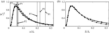
(He, Kazakia & Walker Reference He, Kazakia and Walker1995). As shown in figure 28(b), the mode shapes in the transformed vertical coordinate are nearly the same for flow cases P2 and P3. Hence, for given friction Reynolds number, mean density gradients seem to incorporate well the (small) effects of Mach-number variations. However, differences with respect to the P1 flow case are still present, which may be a consequence of lack of scale separation between the inner and outer layers in P2 and P3.
Optimal log-layer modes for flow cases P1 (corresponding to
 ${\it\lambda}_{z}^{+}=441$
), P2 and P3 (corresponding to
 ${\it\lambda}_{z}^{+}=340$
), taken at
 $t=t_{max}$
. (a) Mode amplitudes as a function of wall distance scaled by spanwise wavelength. (b) Mode amplitudes as a function of density-weighted wall distance scaled by spanwise wavelength. In panel (a) the vertical lines denote the density-averaged wall-normal positions associated with
 ${\tilde{y}}^{+}=20$
and
 ${\tilde{y}}^{+}=100$
for P1–P3. Refer to table 1 for line nomenclature.

It is clear that, based on the present data, making definite statements regarding Reynolds- and Mach-number effects on log-layer modes is quite difficult, mainly given the limited range of available Reynolds numbers, and the difficulty of changing the two parameters separately. It is also far from clear which Reynolds number should be kept constant to isolate ‘compressibility’ from ‘Reynolds-number’ effects. Hence, a much more complete dataset would be needed to further strengthen or refute our findings.
4. Conclusions
The evolution of coherent structures in compressible turbulent boundary layers with free-stream Mach number from 0.2 to 4 has been analysed. The approach relies on optimal transient growth analysis whereby the linearized evolutionary equations of the organized structures are obtained by extending to compressible flows the triple decomposition procedure developed by Reynolds & Hussain (Reference Reynolds and Hussain1972) for strictly incompressible flow. A linear dynamical system results for the organized (coherent) motions, which is closed by prescribing the mean field, and introducing an isotropic eddy viscosity model to describe the turbulent transport of momentum and internal energy by the large scales. For closure purposes the DNS database of Pirozzoli & Bernardini (Reference Pirozzoli and Bernardini2011) has been used for the supersonic flow cases, whereas the explicit closures of Monkewitz et al. (Reference Monkewitz, Chauhan and Nagib2007) have been used for the subsonic cases, here mainly considered for validation purposes. Although closure models based on the assumption of isotropy may suffer from some shortcomings, they nevertheless can also serve as a basis to compare our results with previous incompressible analyses Cossu et al. (Reference Cossu, Pujals and Depardon2009).
An optimal transient growth analysis has been developed based on the definition of an energy norm containing the contributions of both kinetic energy and internal energy. Optimal transient modes have been calculated for a wide range of streamwise and spanwise wavenumbers, with the main finding that absolute optimal modes are always two-dimensional. Optimal modes naturally split themselves into two families, scaling in inner and outer units, respectively, as previously also found in the incompressible regime (Cossu et al. Reference Cossu, Pujals and Depardon2009), and consistent with the two-layer nature of turbulent wall layers. The scale separation effect is here found to be mainly dependent on the friction Reynolds number, rather than on the Mach number. In the intermediate range of spanwise wavenumbers, the maximum growth attains a plateau at all Mach numbers, as also found in incompressible channel flow (del Alamo & Jiménez Reference del Alamo and Jiménez2006). In this region, the optimal structures are mainly localized in the log layer.
Regarding the inner-layer modes, near collapse of the typical spanwise size of the most amplified modes is observed across the Mach-number range, with an absolute peak occurring at
 ${\it\lambda}_{z}^{+}=81.5$
, which matches well the value expected from the near-wall streaks, thus supporting their universality. A similar pattern is observed for the temperature component of the transient growing modes, which is found to be negatively correlated with the streamwise velocity component. The lift-up mechanism underlying the formation of velocity/temperature streaks is explained in terms of vorticity transfer from the streamwise to the spanwise component. As predicted by the classical Morkovin hypothesis, we find that amplitude changes with the Mach number can be effectively compensated through the use of density scaling. Furthermore, the variation of the optimal growth rate with the Mach number is found to be mainly an additive effect linked to increased aerodynamic heating. Hence, no major dynamical effect of compressibility on the mechanisms of transient growth is observed, at least at the Mach numbers under scrutiny. This behaviour is consistent with observations based on DNS (Bernardini & Pirozzoli Reference Bernardini and Pirozzoli2011b
; Pirozzoli & Bernardini Reference Pirozzoli and Bernardini2011).
Amplified modes that populate the outer part of the wall layer have also been identified. Absolute optimal growth is attained by coherent structures that are infinitely elongated in the streamwise direction, and having spanwise size
 ${\it\lambda}_{z}\approx 8.5{\it\delta}$
. This mode is found to be a robust feature, being very weakly dependent on the Reynolds number and on the Mach number. As for the inner peak, a lift-up mechanism is responsible for the growth of the absolute optimal mode, with a similar transfer of vorticity from the streamwise to the spanwise components. All these features agree well with those observed in the incompressible limit (Cossu et al.
Reference Cossu, Pujals and Depardon2009). As in the inner layer, a passive role of temperature is highlighted, and increasing internal energy contribution to the total energy budget is observed. Besides the absolute (two-dimensional) optimal modes, we have also characterized the structure of the three-dimensional modes corresponding to given streamwise and spanwise spatial scales. The general conclusion is that smaller coherent structures have higher inclination angles with respect to the wall, as compared to larger eddies.
Regarding the most amplified log-layer optimal modes, we show that they are streamwise uniform, and exhibit a self-similar behaviour. In particular, both vertical size and characteristic time scale vary linearly with the spanwise wavelength. This observation leads to the conclusion that the idea of geometrically similar attached eddies proposed by Townsend (Reference Townsend1976) also applies to supersonic boundary layers. Furthermore, a universal behaviour of optimal log-layer modes is suggested when accounting for the effects of mean density variations. However, further investigations at higher Mach number and higher Reynolds number are needed in order to draw firm conclusions. The fundamental issue that may be raised regarding the present study is whether the optimal growing modes educed through the linear analysis have physical significance. Regarding the inner-layer modes, it is far from questionable that the absolute optimal modes have strong similarity with coherent structures observed in experiments and DNS, which are in fact mainly elongated in the streamwise direction, and have a spanwise size of the order of 100 wall units. Much less clear is the relevance of the observed outer-layer transient growing modes. In fact, large discrepancies exist between the absolute optimal outer modes and the superstructures that populate the outer part of turbulent boundary layers. For instance, the amplitude of the outer optimal modes is reached at the edge of the boundary layer, whereas very-large-scale outer eddies are mainly energetic at a distance of approximately
 $0.3{\it\delta}$
from the wall (Hutchins & Marusic Reference Hutchins and Marusic2007). Furthermore, both the spanwise and the streamwise size of the absolute optimal outer modes is much larger than for eddies educed in DNS and experiments. However, a host of transient growing modes exist other than the absolute optimal ones, which has not been analysed in detail before. In particular, for boundary layers at
 $\mathit{Ma}_{\infty }=2$
we identify optimal modes having
 ${\it\lambda}_{x}\approx 2.3{\it\delta}$
and
 ${\it\lambda}_{z}\approx 1.5{\it\delta}$
(close to the typically quoted eddy integral length scales), which have a typical inclination angle of approximatively
 ${\it\theta}_{xy}\approx 15^{\circ }$
with respect to the streamwise direction, and which also exhibit anticorrelation between the streamwise and the temperature component.
Our findings seem to support the view that very-large-scale structures in supersonic turbulent boundary layers are the result of an autonomous self-sustained process associated with the amplification and regeneration of optimal modes, rather than the agglomeration of smaller structures (Hwang & Cossu Reference Hwang and Cossu2010b ). However, our analysis admittedly fails to describe the underlying selection mechanism of the most representative mode. In fact, even though modes resembling the ‘real’ ones are recovered among the many suboptimal three-dimensional modes, the most amplified outer mode is still much different from the typical structures observed in turbulent wall layers. In our understanding, this is an inherent limitation of linear analysis, as structures that are selected in physical reality are the eventual result of nonlinear effects and/or secondary instability processes, which are necessarily disregarded by modal analysis.
Regarding the effects of the free-stream Mach number, the general conclusion that can be drawn from the present data is that they are typically small and confined to increasing the amplitude of the temperature fluctuations, while the kinematic field is virtually unaffected. In particular, compressibility effects are seen to be mainly a consequence of changes in the mean density. In this sense, the present results provide further confirmation of the validity of Morkovin’s hypothesis, at least up to
 $\mathit{Ma}_{\infty }=4$
, which is the upper limit investigated here. Notably, this result is at odds with the classical results of linear stability analysis of laminar boundary layers, which shows distinctly different nature of supersonic boundary layers with respect to their low-speed counterpart, also as far as the transition process is concerned (Reshotko Reference Reshotko1976). Studies of transient growth at yet higher Mach number are of course desirable to establish the possible onset of genuine compressibility effects.
We believe that further verification of the robustness of optimal modes computed here can be obtained by considering more accurate modelling of the terms requiring closure, and in this sense full usage of the DNS data may be considered in future work. Specifically, some effort is currently in progress regarding the analysis of different terms involved in the evolution equations for the oscillating background Reynolds stress. We believe that, in perspective, the application of the present structural approach to more complex flows, such as supersonic inlets and shock wave–turbulent boundary layer interactions, could be considered to develop low-order models that accurately describe the organized part of the motion, thus opening interesting avenues to flow control.
Acknowledgements
We acknowledge that some of the results reported in this paper have been achieved using the PRACE Research Infrastructure resource FERMI based at CINECA, Casalecchio di Reno, Italy, and the HPC resources of IDRIS and CCRT under the allocation x20142a7151 by GENCI (Grand Equipement National de Calcul Intensif).
Appendix A. Linearized equations for parallel flows
The governing linear equations for the mode amplitude vector
 $\boldsymbol{q}^{\prime }$
are
 $$\begin{eqnarray}\displaystyle & & \displaystyle \frac{\partial {\it\rho}^{\prime }}{\partial t}+\text{i}{\it\alpha}({\it\rho}^{\prime }\widetilde{u}+\overline{{\it\rho}}u^{\prime })+\frac{\partial \overline{{\it\rho}}v^{\prime }}{\partial y}+\text{i}{\it\beta}\overline{{\it\rho}}w^{\prime }=0,\end{eqnarray}$$
 $$\begin{eqnarray}\displaystyle & & \displaystyle \frac{\partial \overline{{\it\rho}}u^{\prime }}{\partial t}+(\text{i}{\it\alpha}\overline{{\it\rho}}\,\widetilde{u}u^{\prime })+\left(\overline{{\it\rho}}v^{\prime }\frac{\text{d}\widetilde{u}}{\text{d}y}\right)\nonumber\\ \displaystyle & & \displaystyle \qquad =-\text{i}{\it\alpha}p^{\prime }+\left[{\it\mu}_{tot}(-2{\it\alpha}^{2}u^{\prime })-\frac{2}{3}{\it\mu}_{tot}\left(-{\it\alpha}^{2}u^{\prime }+\text{i}{\it\alpha}\frac{\partial v^{\prime }}{\partial y}-{\it\alpha}{\it\beta}w^{\prime }\right)\right]\nonumber\\ \displaystyle & & \displaystyle \qquad +\,\frac{\partial }{\partial y}\left[{\it\mu}_{tot}\left(\frac{\partial u^{\prime }}{\partial y}+\text{i}{\it\alpha}v^{\prime }\right)\right]+{\it\mu}_{tot}(-{\it\beta}^{2}u^{\prime }-{\it\alpha}{\it\beta}w^{\prime }),\end{eqnarray}$$
 $$\begin{eqnarray}\displaystyle & & \displaystyle \frac{\partial \overline{{\it\rho}}v^{\prime }}{\partial t}+(\text{i}{\it\alpha}\overline{{\it\rho}}\widetilde{u}v^{\prime })\nonumber\\ \displaystyle & & \displaystyle \quad =-\frac{\partial p^{\prime }}{\partial y}+{\it\mu}_{tot}\left(-{\it\alpha}^{2}+\text{i}{\it\alpha}\frac{\partial u^{\prime }}{\partial y}\right)+\frac{\partial }{\partial y}\left[{\it\mu}_{tot}\left(2\frac{\partial v^{\prime }}{\partial y}\right)-\frac{2}{3}{\it\mu}_{tot}\left(\text{i}{\it\alpha}u^{\prime }+\frac{\partial v^{\prime }}{\partial y}+\text{i}{\it\beta}w^{\prime }\right)\right]\nonumber\\ \displaystyle & & \displaystyle \qquad +\,{\it\mu}_{tot}\left(-{\it\beta}^{2}v^{\prime }+\text{i}{\it\beta}\frac{\partial w^{\prime }}{\partial y}\right)\end{eqnarray}$$
 $$\begin{eqnarray}\displaystyle & & \displaystyle \frac{\partial \overline{{\it\rho}}w^{\prime }}{\partial t}+(\text{i}{\it\alpha}\overline{{\it\rho}}\widetilde{u}w^{\prime })\nonumber\\ \displaystyle & & \displaystyle \quad =-\text{i}{\it\beta}p^{\prime }+{\it\mu}_{tot}(-{\it\alpha}^{2}w^{\prime }-{\it\alpha}{\it\beta}u^{\prime })+\frac{\partial }{\partial y}\left[{\it\mu}_{tot}\left(\frac{\partial w^{\prime }}{\partial y}+\text{i}{\it\beta}v^{\prime }\right)\right]+{\it\mu}_{tot}(-2{\it\beta}^{2}w^{\prime })\nonumber\\ \displaystyle & & \displaystyle \qquad -\,\frac{2}{3}{\it\mu}_{tot}\left(-{\it\alpha}{\it\beta}u^{\prime }+\text{i}{\it\beta}\frac{\partial v^{\prime }}{\partial y}-{\it\beta}^{2}w^{\prime }\right),\end{eqnarray}$$
 $$\begin{eqnarray}\displaystyle & & \displaystyle \frac{\partial \overline{{\it\rho}}e^{\prime }}{\partial t}+(\text{i}{\it\alpha}\overline{{\it\rho}}\widetilde{u}w^{\prime })+\left(\overline{{\it\rho}}v^{\prime }\frac{\text{d}\widetilde{e}}{\text{d}y}\right)\nonumber\\ \displaystyle & & \displaystyle \quad =-{\it\alpha}^{2}\frac{C_{p}{\it\mu}_{tot}}{\mathit{Pr}}T^{\prime }+\frac{\partial }{\partial y}\left(\frac{C_{p}{\it\mu}_{tot}}{\mathit{Pr}}\frac{\partial T^{\prime }}{\partial y}\right)-{\it\beta}^{2}\frac{C_{p}{\it\mu}_{tot}}{\mathit{Pr}}T^{\prime }+\left[{\it\mu}_{tot}\left(\frac{\partial u^{\prime }}{\partial y}+i{\it\alpha}v^{\prime }\right)\right]\frac{\partial \overline{u}}{\partial y}\nonumber\\ \displaystyle & & \displaystyle \qquad +\,\left[{\it\mu}_{tot}\frac{\text{d}\overline{u}}{\text{d}y}\right]\frac{\partial u^{\prime }}{\partial y}+{\it\mu}_{tot}\left(\frac{\text{d}\overline{u}}{\text{d}y}\right)\text{i}{\it\alpha}v^{\prime }-\overline{p}\left(\text{i}{\it\alpha}u^{\prime }+\frac{\partial v^{\prime }}{\partial y}+\text{i}{\it\beta}w^{\prime }\right),\end{eqnarray}$$
 $T^{\prime }=e^{\prime }/C_{v}$
and
 ${\it\mu}_{tot}={\it\mu}+{\it\mu}_{t}$
.
Appendix B. Production and dissipation terms
The production and dissipation terms associated with the kinetic energy budget are
 $$\begin{eqnarray}\mathscr{P}^{k}=\displaystyle -\int _{0}^{L_{y}}\overline{{\it\rho}}\frac{\text{d}\overline{u}}{\text{d}y}u^{\prime h}v^{\prime }\,\text{d}y+\text{c.c.},\hspace{170.39996pt}\end{eqnarray}$$
 $$\begin{eqnarray}\displaystyle \mathscr{D}_{v}^{k} & = & \displaystyle \displaystyle -\int _{0}^{L_{y}}~{\it\alpha}^{2}\frac{1}{3}{\it\mu}u^{\prime h}u^{\prime }+{\it\mu}({\it\alpha}^{2}+{\it\beta}^{2})u^{\prime h}u^{\prime }\nonumber\\ \displaystyle & & \displaystyle -\displaystyle \,u^{\prime h}\left(\frac{\text{d}{\it\mu}}{\text{d}y}\frac{\partial }{\partial y}+{\it\mu}\frac{\partial ^{2}}{\partial y^{2}}\right)u^{\prime }-\text{i}{\it\alpha}u^{\prime h}\left[\frac{\text{d}{\it\mu}}{\text{d}y}+\frac{{\it\mu}}{3}\frac{\partial }{\partial y}\right]v^{\prime }\nonumber\\ \displaystyle & & \displaystyle +\,\displaystyle \,{\it\alpha}{\it\beta}u^{\prime h}\frac{{\it\mu}}{3}w^{\prime }-\text{i}{\it\alpha}v^{\prime h}\left[-\frac{2}{3}\frac{\text{d}{\it\mu}}{\text{d}y}+\frac{1}{3}{\it\mu}\frac{\partial }{\partial y}\right]u^{\prime }\nonumber\\ \displaystyle & & \displaystyle +\displaystyle \,{\it\mu}v^{\prime h}({\it\alpha}^{2}+{\it\beta}^{2})v^{\prime }-v^{\prime h}\left[\frac{1}{3}\frac{\text{d}{\it\mu}}{\text{d}y}\frac{\partial }{\partial y}+\frac{1}{3}{\it\mu}\frac{\partial ^{2}}{\partial y^{2}}+\frac{\text{d}{\it\mu}}{\text{d}y}\frac{\partial }{\partial y}+{\it\mu}\frac{\partial ^{2}}{\partial y^{2}}\right]v^{\prime }\nonumber\\ \displaystyle & & \displaystyle -\displaystyle \,\text{i}{\it\beta}v^{\prime h}\frac{1}{3}{\it\mu}\frac{\partial w^{\prime }}{\partial y}+\text{i}{\it\beta}v^{\prime h}\frac{2}{3}\frac{\text{d}{\it\mu}}{\text{d}y}w^{\prime }+{\it\alpha}{\it\beta}w^{\prime h}\frac{1}{3}{\it\mu}u^{\prime }-\text{i}{\it\beta}w^{\prime h}\left[\frac{1}{3}{\it\mu}\frac{\partial }{\partial y}+\frac{\text{d}{\it\mu}}{\text{d}y}\right]v^{\prime }\nonumber\\ \displaystyle & & \displaystyle +\displaystyle \,w^{\prime h}\left[{\it\mu}({\it\alpha}^{2}+{\it\beta}^{2})+{\it\beta}^{2}\frac{1}{3}{\it\mu}-{\it\mu}\frac{\partial ^{2}}{\partial y^{2}}-\frac{\text{d}{\it\mu}}{\text{d}y}\frac{\partial }{\partial y}\right]w^{\prime }\text{d}y+\text{c.c.}\end{eqnarray}$$
A similar expression for
 $\mathscr{D}_{t}^{k}$
is obtained, by replacing
 ${\it\mu}$
with the eddy viscosity.
Laminar supersonic adiabatic boundary layer for
 $\mathit{Ma}_{\infty }=2.5$
,
 ${\it\alpha}=0$
and
 $\mathit{Re}_{{\it\delta}}=2650$
. (a) Distribution of the amplification associated with the total energy as a function of the dimensionless time for
 ${\it\beta}=0.1$
. (b) Distribution of
 $G_{max}$
as a function of
 ${\it\beta}$
. Dashed line, data of Hanifi et al. (Reference Hanifi, Schmid and Henningson1996); full line, a laminar flow is assumed; dotted line, a turbulent flow is assumed with
 ${\it\mu}_{t}=0$
.

Appendix C. Validation of the optimal transient growth code
In order to prove the capability of the present approach to reproduce classical results of stability theory, we have analysed a laminar boundary layer under the same flow conditions as Hanifi et al. (Reference Hanifi, Schmid and Henningson1996), namely
 $\mathit{Ma}_{\infty }=2.5$
,
 $\mathit{Re}_{{\it\delta}}=2550$
, with adiabatic wall. In figure 29(a), we show the growth rate as a function of time for
 ${\it\alpha}=0$
and
 ${\it\beta}=0.1$
, and in figure 29(b) the maximum growth rate as a function of the spanwise wavelength, assuming either laminar flow or fully turbulent flow, whereby the model terms are set to zero. The results confirm the validity of our approach and show that the neglected terms have very limited influence in a laminar regime.