1. Introduction

The agreement of independent measurements occurs when a theoretically posited quantity is measured via multiple and (in some sense) “independent” methods and those measurements agree (cf. Forster Reference Forster1988). The phenomenon is also called “the method of overdetermination of constants” (Norton Reference Norton, Nola and Sankey2000) and “the consilience of inductions” (Whewell Reference Whewell and Butts1989). Judging by the scientific episodes most studied and celebrated by philosophers, the phenomenon is of central importance to confirmation in science. The agreement of independent measurements played a key role in confirming, for example, Newton’s theory of gravity (Forster Reference Forster1988), the wave theory of light (Whewell Reference Whewell and Butts1989), Darwin’s theory of common ancestry (Helgeson Reference Helgeson2013), the atomic theory of matter (Salmon Reference Salmon1984; Norton Reference Norton, Nola and Sankey2000), the charged particle (electron) theory of cathode rays (Norton Reference Norton, Nola and Sankey2000), and the theory of plate tectonics (Koolage Reference Koolage2008). In the present essay I propose a new, formal account of the phenomenon’s epistemic significance and contrast my proposal with a more established approach to the same problem.

The agreement of independent measurements is often treated under the “diversity of evidence” heading (where the “independence” of individual measurements is taken to enhance the “diversity” of a total set of observations that includes those measurements). But that approach (in its current form) does not adequately acknowledge the hierarchical structure that is characteristic of hypothesis spaces in science. Specific scientific hypotheses are nested within more general hypotheses, and those are nested within hypotheses more general still. Within such a structured hypothesis space, the diversity of evidence approach locates the evidential significance of agreeing measurements at the nitty-gritty level of parameter estimates: agreement warrants extra confidence that the measured value is accurate. While not incorrect, this result is incomplete and does little to explain the perceived significance of agreeing measurements in the history of science. My proposal complements existing accounts by identifying, in addition, warrant for the “higher-level” theory that posits the measured quantity. It is the confirmation of this higher-level hypothesis—more so than the very specific hypothesis that a parameter takes a certain value—that explains the historical significance of the real scientific examples.

Regarding formal methodology, I will judge the evidential import of an observation via the law of likelihood (Hacking Reference Hacking1965; Edwards Reference Edwards1984; Royall Reference Royall1997). That is, I take observation o to favor hypothesis over hypothesis iff . Bayesians of all stripes can agree that it is through these probabilities that observations confirm hypotheses. I wish to bracket the finer points about how strongly a hypothesis is confirmed by an observation (Fitelson Reference Fitelson1999); my proposal concerns the more basic issue of exactly which hypotheses and observations to label o, , and such that the import of agreeing measurements can be better appreciated within the framework of Bayesian epistemology broadly understood.

2. The Phenomenon to Be Analyzed

As an example of the phenomenon to be analyzed, consider Whewell’s account of scientific work by Thomas Young: “And what was no less striking a confirmation of the truth of the [wave] theory [of light], Measures of the same element deduced from various classes of facts were found to coincide. Thus the Length of a luminiferous undulation, calculated by Young from the measurement of Fringes of shadows, was found to agree very nearly with the previous calculation from the colours of Thin plates” (Reference Whewell and ButtsWhewell 1858/1989, 154). Whewell is saying that agreement between measurements of the wavelength of light confirms the theory that light is made of waves (as opposed to the hypothesis that light waves have such and such length). Similarly, Norton says of Perrin’s argument for the atomic theory of matter that “Perrin was able to report roughly a dozen different methods for estimating N [Avogadro’s number] and they all gave values of N in close agreement” and that “the case for the reality of atoms and molecules lay in this agreement” (Norton Reference Norton, Nola and Sankey2000, 73).

It is this type of inference—confirmation for the higher-level theory based on agreeing measurements of a quantity posited within the theory—that I will reconstruct formally in what follows. Again, this is not to deny that such agreement can also confirm the measured value for the quantity posited within the theory if that theory is already taken to be true. But Young’s main conclusion was that light is a wave. Perrin’s main conclusion was that matter is made of atoms. (Analogous statements hold for the other examples mentioned above.)

3. Measurement Formally Characterized

To begin my analysis of the agreement of measurements, I first abstractly characterize the phenomenon itself. I formally characterize measurement as the statistical procedure of parameter estimation. Parameter estimation requires a statistical model—a family of probability distributions, each associated with a particular value for the model’s adjustable parameter (or with a vector of values if the model has multiple parameters). Given a set of data, the highest-likelihood distribution (or distributions) within the family can be identified, and the associated parameter value (or interval) is the parameter estimate. On this characterization of measurement, the statistical model’s adjustable parameter is the quantity to be measured, and estimation of that parameter’s value, as just described, is a measurement. For example, suppose that we want to measure the mass of an object using a spring scale. Like any measuring device, our scale is imperfect. Suppose that its readings are normally distributed around the true mass of the object that is hung from it. This supposition is the statistical model. We produce a set of data by hanging the object, observing the reading, removing the object, then repeating the procedure a number of times. These data are then used to estimate the mean of the normal distribution from which the individual readings were treated as random draws. This estimate is a measurement of the object’s mass.

What then, is the agreement of measurements? Suppose that we have two disjoint data sets and a statistical model for each. The two models need not be the same, and each may include adjustable parameters that the other does not, but they must both contain an adjustable parameter representing the quantity to be measured. Each model is fitted to its respective data set, generating two vectors of parameter estimates and two estimates of the shared parameter, that is, two measurements of the quantity to be measured. Continuing with the spring scale example, suppose that we measure the mass of the same object again, this time (as astronauts are “weighed” in space) by applying a known force, observing the object’s motion, and working back to its mass through . In this case the data are (position, time) points, and the statistical model is a Newtonian equation of motion with a stochastic element representing observation error. The resulting estimate of m is a second measurement of the object’s mass. (I understand agreement as a matter of degree, and I quantify this precisely in the worked example below.)

4. Agreement as Observation

With the phenomenon formally characterized, I turn to its epistemic significance. I first illustrate my approach using the simplest possible case of the agreement of measurements. Say we will make two measurements of the mass of an object, using two separate spring scales. Let there be two data sets with 20 points each, and , corresponding to 40 scale readings, 20 from each scale, all using the same object. For each data set employ the location-normal model with known variance and unknown mean . That is, model a says that the 20 points are drawn from 20 independent and identically distributed random variables , each normal with variance and mean . Model b says the same about points , with mean . Under the location-normal model, the maximum likelihood estimator of is the mean of the data set. So the two maximum likelihood estimates for the true values of and are and , respectively.

Now I introduce a supermodel that expresses the assumption, required for the agreement of measurements, that and are two estimates (measurements) of the same quantity. This supermodel is the location-normal model treating all 40 random variables as independent, normal distributions, each with variance and mean . And to quantify the degree of agreement between the two measurements of the parameter , I define the following statistic of the total data set : . The closer this statistic is to zero, the greater the agreement between measurements. Call this the agreement statistic.Footnote ¹ What does the supermodel predict about the value of the agreement statistic? With respect to the supermodel, this particular statistic is what is called ancillary, meaning that the distribution for the statistic under the model does not depend on the adjustable parameter. 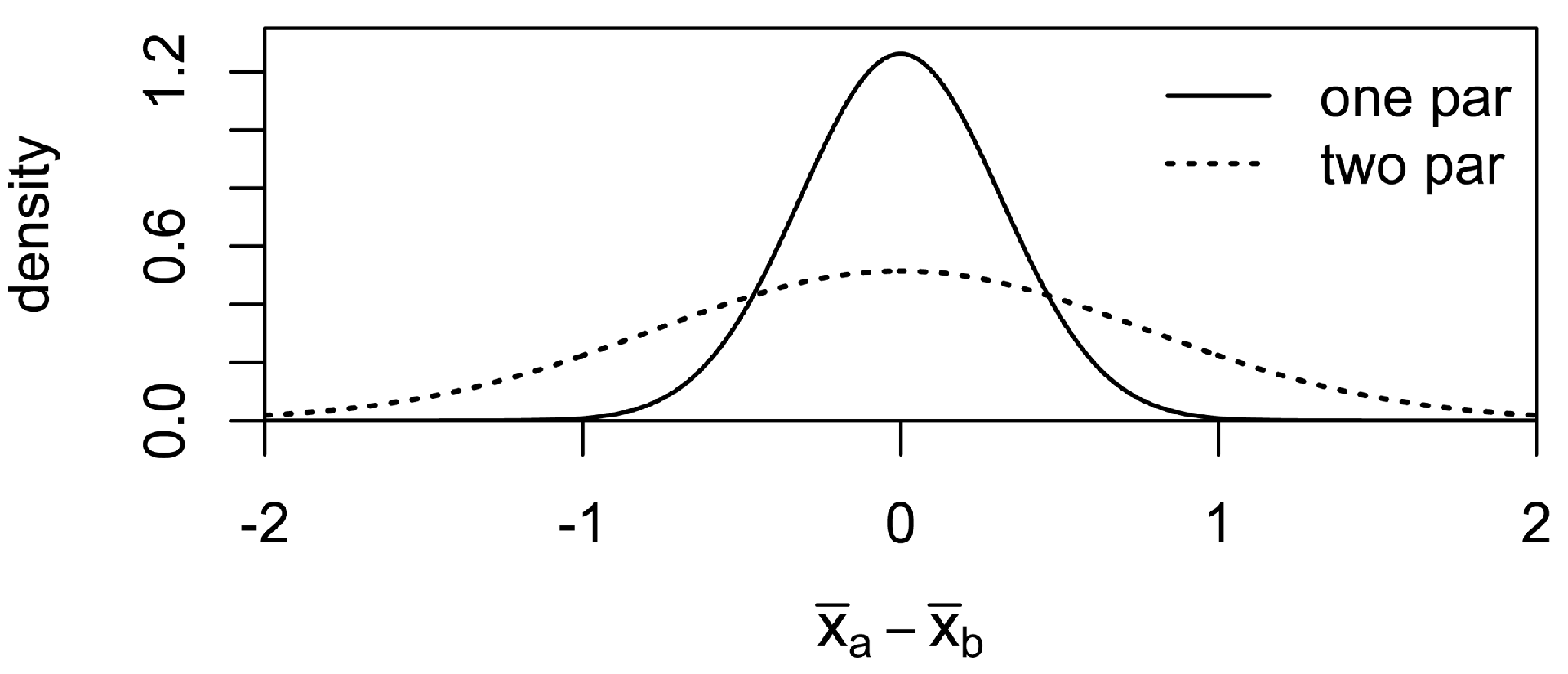This is easy to understand intuitively since if all 40 random variables have the same distribution, then we can predict that and will cluster around roughly the same value (), even without knowing what that value will be. So the supermodel should assign higher probability to values of the agreement statistic near zero and lower probability to large positive or negative values. The actual distribution is shown as the solid line in figure 1.

Figure 1.

Probability density distributions for the agreement statistic under the one-parameter and two-parameter supermodels.

To summarize what I have done so far, I first treat measurement as parameter estimation and the agreement of measurements as agreement between two estimates, based on disjoint data sets, of a single parameter shared by two statistical models. To formally encode the idea that the parameter appearing in both statistical models is the same quantity, I introduce a supermodel that posits a single parameter underlying all 40 data points. Then I characterize the agreement of measurements as a statistic of the total data (in this case ) and I treat the degree of agreement itself as an observation. I must emphasize this last part because it is the key to my approach. It may initially seem unintuitive (or worse) to treat the degree of agreement between two estimates of a posited quantity as an observation. Admittedly, it is an abstract, “high-level” observation. Yet the agreement statistic is a straightforward function of the total data set and is thus entirely determined by the data.Footnote ² And as long as we can calculate a probability function for the statistic, nothing prevents us from treating it as an observation within our statistical framework. For my simplest-case example, I have displayed the probability distribution assigned to the agreement statistic by the supermodel. My next step is to introduce a competing supermodel and calculate the distribution that it assigns to the same agreement statistic. I will then locate the epistemic significance of the agreement of independent measurements in the likelihood favoring of the one supermodel over the other, given observed values of the agreement statistic near zero.

5. A Competing Supermodel

I want the competing supermodel to lack the commitment to and estimating the same theoretically posited quantity, so rather than positing a single parameter underlying all the data, I let the alternative supermodel be a composite of the two separate location-normal models (one for and one for ), retaining both parameters and . Call the original supermodel the one-parameter supermodel and call the alternative the two-parameter supermodel.

What does the two-parameter supermodel say about the agreement statistic ? Unlike the previous case, the statistic’s distribution under the two-parameter supermodel does depend on the parameters. On its own, the two-parameter supermodel does not say enough—it is too logically weak—to predict anything about that statistic. We can, however, use a standard Bayesian technique to generate a distribution over the agreement statistic by logically strengthening the two-parameter supermodel hypothesis. We can assume prior probability distributions for the parameters and and then “integrate out” those priors. Think of this logically strengthened hypothesis as describing a two-layered stochastic process. The data are generated by first drawing values for and from their respective prior distributions and then drawing data points and from normal distributions with means and , respectively. The first layer is intended to represent uncertainty about the true values of the parameters, and the two-layered process incorporates that uncertainty into the supermodel’s predictions about the data. Adding priors in this way logically strengthens the two-parameter supermodel enough to generate a distribution over the agreement statistic, and I employ this procedure in order to contrast the two supermodels vis-à-vis observed values of that statistic.

Exactly what the augmented two-parameter supermodel predicts about the agreement statistic of course depends on what priors are built into that hypothesis. But qualitatively, the likelihood comparison between the two supermodels is not very sensitive to the choice of priors. Here is one example calculation. For convenience, suppose that the priors for and are normal, and in accord with the intent of the two-parameter supermodel, let them be independent. A variance of for each will represent a moderate degree of uncertainty. The distribution over the agreement statistic further depends only on the difference between the means of the two priors, not on the means themselves. A difference of zero is most advantageous for the two-parameter supermodel (but will not destroy the contrast I wish to draw). The resulting distribution is shown as the dotted line in figure 1.Footnote ³

A comparison of the two distributions pictured in figure 1 shows that the one-parameter supermodel has the higher likelihood for observed values of the agreement statistic near zero. It is this likelihood comparison between the two supermodels that, on my account, expresses the evidential significance of the agreement of independent measurements.

6. Application

So far I have provided a concrete illustration, framed in abstract mathematical terms. It remains to be explained how the competing hypotheses that are salient within the real scientific episodes characterized as “the agreement of independent measurements” are relevantly similar to the two supermodels from my illustration.

The real-world analogues of the one-parameter supermodel are hypotheses that posit a quantity that is not (colloquially speaking) directly observable but can (according to its hypothesized nature) be measured in multiple ways. For example, in Newton’s physics the mass of an object can be measured by observing how much the object stretches a spring or by observing how much it accelerates when a force is applied. Likewise, the wave theory of light posits a wavelength, and the atomic theory of matter posits a number of particles in a standard unit of a substance. Each posited quantity was (eventually) measurable in a variety of ways. These are the one-parameter hypotheses.

The real-world analogues of the two-parameter supermodel are harder to characterize as a group since these hypotheses vary a great deal in how fully and explicitly they are articulated. They lie on a scale from full-fledged alternative scientific theory to vague skeptical worry. Despite the variation exhibited in that dimension, I will endeavor to explain how they all share the relevant similarity to the two-parameter supermodel from my illustration. To do this, I must go back and discuss an aspect of my formal illustration that I glossed over in the first pass.

Returning to the formal illustration, consider the dual nature of the quantity , the mean value of the data set . On the one hand, is the maximum likelihood estimate of the value of the parameter . Call this the theoretical perspective on . But at the same time, is merely the result of a mathematical operation applied mechanically to the data set . Call this the observational perspective on . Notice that while the two supermodels share the same observational perspective on , they take different theoretical perspectives. We might say that they offer different interpretations of . The one-parameter supermodel interprets as the best estimate of the single parameter that underlies all the data . The two-parameter supermodel interprets as the best estimate of the parameter (which parameter has no bearing on the second data set ). The common thread among real-world analogues of my two-parameter supermodel is that those hypotheses offer more limited, local interpretations of a single measurement.

On the full-fledged scientific theory end of the spectrum, take, for example, the Ptolemaic theory of the solar system as an alternative to the Copernican theory. Ptolemy put the earth at the center of the solar system and decomposed the apparent motion of each planet (as viewed from the earth) into an orbit around the earth (the deferent) plus a second, smaller orbit (the epicycle) that circles a point moving along the deferent. It turns out that the Ptolemaic epicycle captures the component of apparent planetary motion that is in fact contributed by the motion of the earth around the sun. In effect, Ptolemy (unknowingly) took the motion of the earth around the sun and displaced it to another location within his picture of the solar system—but another location from which it could make the same contribution to the overall motion of a planet relative to the earth. Thus the relative motion of the sun and earth is replicated within the Ptolemaic model for each planet. A Ptolemaic supermodel addressing two planets plus the earth will then include one parameter for the period of the first planet’s epicycle and another parameter for the period of the second planet’s epicycle. The corresponding Copernican supermodel, however, will treat the estimates of those two parameter values as two estimates of the same quantity, namely, the period of the earth’s orbit around the sun.

At the other end of the spectrum we have less fully articulated ideas about a measurement being an “artifact” of the measuring procedure, the measuring device, or the particular experimental setup generating the data (cf. Hacking Reference Hacking, Churchland and Hooker1985). The single-parameter hypothesis interprets the measurement as an estimate of a property of the entity under study, which property will naturally be constant across repeated measurements or measurements using different techniques. The alternative hypothesis interprets the measurement as a property of the dust on the microscope lens, of a glitch in the computer software, or of a one-off spike in emissions from the factory down the road, that is, as an estimate of some quantity that is of less general significance and would not be expected to influence attempted measurements of the target property on other occasions or through other media. Fully articulating such alternative hypotheses would involve positing separate parameters underlying the results of separate measurement attempts on other occasions or through other media, as per the two-parameter supermodel in my illustration.

7. Independence

Insofar as the account given here furnishes an analysis of “independence,” measurements are independent where any among the competing hypotheses fail to interpret those measurements as estimates of a single quantity. This is, in any case, the feature of the hypothesis space that is ultimately responsible for the likelihood contrast displayed in figure 1, and we can treat the “independent” in “agreement of independent measurements” as flagging this feature.Footnote ⁴ To better situate my account with respect to existing literature, I contrast it with a more established approach to independent evidence. The important point of contrast will be not so much the particular meaning of “independence” (though this too is different), but rather the inference problem to which independent evidence is taken to be relevant.

The intuitive notion of “independent” evidence (or perhaps there is more than one) overlaps with that of observations being “of different kinds.” And where a set of observations has parts deemed independent (or different in kind), that set is often called “diverse” or “varied.” Within Bayesian epistemology, there is a standard approach to all these terms, exemplified (among other places) in Hempel’s discussion of the “criteria of confirmation and acceptability.” Hempel first remarks that “broadly speaking, the increase in confirmation effected by one new favorable instance will generally become smaller as the number of previously established favorable instances grows,” before quickly adding a caveat: “If the earlier cases have all been obtained by tests of the same kind, but the new finding is the result of a different kind of test, the confirmation of the hypothesis may be significantly enhanced. For the confirmation of a hypothesis depends not only on the quantity of the favorable evidence available, but also on its variety: the greater the variety, the stronger the resulting support” (Hempel Reference Hempel1966, 33–34). Hempel is here addressing a set of observations each of which individually confirms the hypothesis in question and then gesturing at a notion of variety within such sets and a relationship between this variety and the sum total of confirmation provided by the set.Footnote ⁵

In my example above, the “independent” observations are and . What hypothesis is favored by each of those observations considered individually? We have so far had no use for a prior on the parameter , and consequently, the likelihood of the one-parameter supermodel, given either observation, is undefined. So we cannot say that either observation favors one supermodel over the other. We can, of course, supplement the one-parameter supermodel with a prior distribution over and integrate out to arrive at probabilities for and conditional on that supermodel. But supposing that we choose the same prior for and (as would seem to facilitate a fair contest), the two supermodels will assign exactly the same probability to the observation (and to any other statistic of ). If we instead choose different priors for and , then the observation may favor one supermodel over the other, but this will be due entirely to the choice of priors, with no general validity. The same can be said, mutatis mutandis, of the second observation, . (In terms of the spring scale example, one hypothesis says that two scales measure the same property of an object, while the other says that they measure two different properties, or at least may do so. Naturally, weighing an object on only one of the scales does not discriminate between the two hypotheses.)

To find a hypothesis that is favored by each measurement considered individually, we must set aside the two-parameter supermodel and look within the one-parameter supermodel, to hypotheses about the parameter . When and agree, each observation favors parameter values near the agreed-on number over those further away (recall that is the maximum likelihood estimate of ). Thus, the standard approach to independence and variety points us to hypotheses about the parameter within the one-parameter supermodel, whereas the focus of my approach is the supermodel itself.

When this distinction is mapped back onto the motivating scientific examples, the standard approach to independence and diversity presupposes the wave theory of light and then asks how diversity among measurements helps confirm a value for the wavelength. The standard approach presupposes the atomic theory of matter and addresses the confirmation of hypotheses about the size of the atom, and so on for the other examples. In contrast, I have tried to show how agreement between measurements of the wavelength of light can evidentially favor the wave theory of light over certain alternatives (and, through this, confirm the theory), how agreement between measurements of the size of the atom can favor the atomic theory of matter over alternatives, and so on.

8. Conclusion

Seeing that multiple, “independent” measurements of a quantity agree, one intuitive conclusion is that the value about which the measurements agree is correct (and, moreover, the greater the independence, the more confidence is warranted). But there is another, more basic (yet less obvious) conclusion, which is equally intuitive once made explicit: that the several procedures used for measurement in fact measure the same property. The first conclusion, which is the subject of the diversity of evidence literature, presupposes the second. I have pointed to historically detailed philosophical work suggesting that the second conclusion is at least as important as the first within the scientific episodes that are described as the agreement of independent measurements and partially motivate the diversity of evidence literature. I have provided a template for formal reconstruction and rationalization of this second and more basic element within the motivating scientific episodes. The key innovation is to treat the degree of agreement between measurements as a single observation (a statistic of a total data set). Hypotheses that posit a single property underlying multiple measurement attempts will tend to assign a higher probability to close agreement between measurements, as compared to hypotheses that posit different parameters underlying different measurement attempts.