





1. Introduction
Theoretical and numerical studies of electrosprays in cone-jet mode available in the literature have been performed on the basis of macroscopic electro-hydro-dynamic (EHD) models where electrokinetics is not considered (Gañán-Calvo, Barrero & Pantano Reference Gañán-Calvo, Barrero and Pantano1993; Fernandez de la Mora & Loscertales Reference Fernandez de la Mora and Loscertales1994; Gañán-Calvo Reference Gañán-Calvo1997; Hartman et al. Reference Hartman, Brunner, Camelot, Marijnissen and Scarlett1999; Higuera Reference Higuera2003; Collins et al. Reference Collins, Jones, Harris and Basaran2008; Herrada et al. Reference Herrada, Lopez-Herrera, Gañan-Calvo, Vega, Montanero and Popinet2012; Gamero-Castaño & Magnani Reference Gamero-Castaño and Magnani2019). These models do not describe in detail the concentrations of the species involved in the electrokinetic processes, but rather the net charge resulting from the excess of the charged species. In particular, in these EHD models the electric current due to an external electric field is assumed to be proportional to the latter according to Ohm's law. The proportionality constant, the conductivity  $\kappa$, is therefore in these models a physical property to be characterized (or measured) and is usually assumed to be uniform and constant within the fluid. In contrast, in an electrokinetic approach, the conductivity turns out to be a macroscopic variable that reflects the combined capacity of all charged species to migrate by the action of the electric field within the fluid. Therefore, the proportionality of the electric current to the electric field would be homogeneous provided that the concentrations of the charged species were also homogeneous.
In the simplest EHD model, the Taylor and Melcher leaky dielectric model (LDM), the bulk of the fluid is assumed to be neutral, and charge imbalances occur at the fluid interfaces only. In the LDM, therefore, the relevant variable is the resulting surface charge density, which should obey a surface conservation equation involving surface deformation, convection and charge injection from the bulk. Surface charge convection can be neglected in the LDM provided the fluid flow does not alter significantly the surface charge distribution (Taylor Reference Taylor1966). However, its incorporation is essential in problems with intense electric fields and/or collapsing flows around geometrical singularities, where intense accelerations and decelerations may occur. Examples of these problems are the flow around the vertex of the Taylor cone in electrospray (Gañán-Calvo et al. Reference Gañán-Calvo, Lasheras, Dávila and Barrero1994), around the poles of a droplet (Collins et al. Reference Collins, Sambath, Harris and Basaran2013) or around its equator (Brosseau & Vlahovska Reference Brosseau and Vlahovska2017) under a variety of circumstances and boundary conditions. The only electrical stresses considered in this model are established at the fluid interface. The LDM is justified by the predominance and immediacy of the charge ohmic migration that flattens the charge inhomogeneities in the fluid bulk. That is, LDM is suitable when the characteristic electrical relaxation time,  $t_e \sim \varepsilon /\kappa$, where
 $\varepsilon$ is the fluid electrical permittivity, is much shorter than any hydrodynamic time
 $t_h$ that may be involved, i.e.
 $t_e \ll t_h$. The LDM has been successfully employed to simulate the electrospray cone-jet mode. In particular, it is the model of choice in the theoretical and numerical characterizations available in the electrospray literature, and has been broadly validated by experiments.
Several approaches follow after the simplifications adopted, ranging from a strict electrokinetic approach (López-Herrera et al. Reference López-Herrera, Gañán-Calvo, Popinet and Herrada2015) requiring the characterization of the species involved at the molecular scale by means of the Poisson–Nernst–Planck (PNP) equations up to a macroscopic model of maximum simplicity such as the LDM, in which the relevant variable is the surface charge density  $\sigma _e$, and the electrokinetics is reduced to a homogeneous macroscopic physical property such as the electrical conductivity
 $\kappa$.
Among the models that consider non-zero volumetric charges, the simplest EHD approach considering bulk charges is the one formulated in terms of the volumetric charge density  $\rho _e$, which encompasses all ionic concentrations present. Here,
 $\rho _e = \sum _k z_k e n_k$, where
 $e$ is the charge of an electron and
 $z_k$ and
 $n_k$ are the valence and concentration of the
 $k$th ionic species (the concentrations are defined here as number of ions per unit of volume). To obtain a closed model, thermal diffusion phenomena are generally neglected compared with electrical drift migration, at the expense of a gross (integral) modelling of the Debye layer where thermal diffusion is relevant. This lack of accuracy in the charge distribution does not seriously compromise the model as long as the layer thickness is small compared with all other relevant hydrodynamic lengths, as it still allows a consistent integral (volumetric) formulation of the conservation of charges across the interface. This is the model used in open source numerical schemes employing volumes of fluids (VoF) such as Gerris or Basilisk (López-Herrera, Popinet & Herrada Reference López-Herrera, Popinet and Herrada2011).
In the LDM, the diffuse three-dimensional Debye layer of thickness  $\lambda _D$ is replaced by a discontinuous two-dimensional surface charge density
 $\sigma _e$ related to the jump of electric displacements through the layer as
 $\sigma _e= \varepsilon _1 E_{n,1}- \varepsilon _2 E_{n,2}$, where subindices
 $1,2$ indicate the domains sharing the interface, and
 $E_n$ are the normal components of the electric fields at the interface. The surface charge is involved in two balances: (i) the momentum balance at the surface through the resulting Maxwell electrostatic stresses, and (ii) the charge conservation on a moving surface that may additionally receive or lose charges from the bulk by conduction. The Taylor–Melcher LDM is instituted as the benchmark EHD model after its success in predicting the deformations of a poorly conducting drop suspended in a quasi-dielectric atmosphere by the action of an external uniform electric field (Taylor Reference Taylor1966). Employing the electrified suspended droplet as a benchmark problem, Baygents & Saville (Reference Baygents and Saville1990), Zholkovskij, Masliyah & Czarnecki (Reference Zholkovskij, Masliyah and Czarnecki2002), Schnitzer & Yariv (Reference Schnitzer and Yariv2015) and Mori & Young (Reference Mori and Young2018) sought to bridge the gap between electrokinetics and simplified EHD models by seeking a rigorous derivation of the LDM from the PNP equations.
Schnitzer & Yariv (Reference Schnitzer and Yariv2015) culminated the work of Baygents & Saville (Reference Baygents and Saville1990) by proving, through a rigorous scaling analysis, that the LDM is a consistent electrokinetic limit if the following is satisfied:
 \begin{equation} 1 \ll \beta_s = \frac{\varPhi_a}{\varPhi_T} \ll \frac{1}{\delta_s} = \frac{L_c}{\lambda_D},\end{equation}
where  $L_c$ is a characteristic length,
 $\varPhi _a$ is the order of magnitude of the applied voltage and
 $\varPhi _T = K_b T/e$ is the thermal voltage that results from combining the Boltzmann constant
 $K_b$, the temperature
 $T$ and the elementary charge of an electron
 $e$. Here,
 $\varPhi _T$ is of the order of 26 mV. Expression (1.1) implies three fundamental requirements:
(i)
 $\delta _s \ll 1$ (i.e. $L_c\gg \lambda _D$) is a geometrical requirement that reflects the interfacial character of the LDM.
(ii) The constraint
$\beta _s \gg 1$ (i.e. $\varPhi _a \gg \varPhi _T$) indicates that in EHD problems the applied voltage is well above the thermal voltage.(iii) Finally,
$\beta _s \delta _s \ll 1$ (i.e. $\varPhi _a/L_c \ll \varPhi _T/\lambda _D$) implies the assumption that the outer electric field ($\sim \varPhi _a/L_c$) does not alter the Debye layer (implying local fields $\sim \varPhi _T/\lambda _D$).


Under these conditions, the theoretical analysis of Schnitzer and Yariv leads to the same results as the LDM in the absence of surface charge convection. In addition, they also consider strong binary electrolytes in which the ions are fully dissociated. Furthermore, the generality of the analysis is also compromised by the assumption of (i) a nearly spherical geometry, (ii) the proportionality between ion diffusivity and viscosity regardless of the solvent used (the so-called Walden rule) and (iii) the absorption of ions at the interface that results in the existence of a surface concentration. This surface concentration is related to the volumetric concentrations through adsorption/desorption coefficients.
The approach of Mori & Young (Reference Mori and Young2018), although preserving the scaling (1.1), is very different from Schnitzer & Yariv (Reference Schnitzer and Yariv2015) as it establishes that the slight conductive character of the fluids modelled by the LDM must be linked to the dominant presence of a neutral species with a weak dissociability, which generates a small amount of ions in contrast to the negligible concentration of neutral species in the formulation of Schnitzer and Yariv that assumes a completely dissociated fluid. The reaction terms are therefore maintained in the PNP equations and the concentration of the neutral species must be taken into account in the original equations. The complete dissociation of the neutral species is characteristic of solvents of high polarity, while electrolytes often hardly dissolve in low permittivity solvents, thus behaving as weak electrolytes of dominant neutral species. Other notable differences between Mori's approach and that of Schnitzer and Yariv are the absence, as a simplifying assumption, of surface charge at the interface in the former (absence of adsorbed ions and, therefore, of surface concentrations), the relaxation of Walden's rule (no proportionality between viscosity and ion diffusivity is required) and the presence of surface charge convection in the latter.
However, although the LDM can be advocated as a rigorous limit of a complete electrokinetic model under certain conditions (Schnitzer & Yariv Reference Schnitzer and Yariv2015; Mori & Young Reference Mori and Young2018), to unconditionally adopt it as a general (rigorous) limit of the PNP equations governing ion concentrations in EHD problems is not possible. In effect, despite its enormous success, in sufficiently fast phenomena where volumetric charge convection is expected to be comparable to the volumetric ohmic charge drift, the LDM should be abandoned in favour of volumetric EHD models. In this regard, the electrospray, and in particular (despite its obvious simplification), the steady Taylor cone-jet mode (TCJ), constitutes a paradigmatic EHD problem to test the validity of the different simplifications of the PNP equations. Interestingly, Newtonian liquids with a vast variety of physical properties (electrolytes, ionic liquids, polar and low polarity solvents, mixtures, etc.) obey universal scaling laws within relatively narrow tolerances obtained under the LDM approximation (Gañán-Calvo et al. Reference Gañán-Calvo, López-Herrera, Herrada, Ramos and Montanero2018). Given the still unsettled controversy around the validity of the LDM in every steady TCJ configuration suggested by the rather universal observed validity of scaling laws based on its assumptions (Gañán-Calvo et al. Reference Gañán-Calvo, Barrero and Pantano1993; Fernandez de la Mora & Loscertales Reference Fernandez de la Mora and Loscertales1994; Gañán-Calvo Reference Gañán-Calvo2004; Fernández de la Mora Reference Fernández de la Mora2007), a highly relevant unresolved question is whether a detailed electrokinetic model would lead to results consistent with the LDM. This investigation would shed light on the ultimate reasons of this physical concurrence, providing solid grounds to eventually resolve outstanding challenges in this field such as the physics behind the stability limits of the steady TCJ (Gañán-Calvo, Rebollo-Muñoz & Montanero Reference Gañán-Calvo, Rebollo-Muñoz and Montanero2013) or the initiation dynamics of TCJ (Collins et al. Reference Collins, Jones, Harris and Basaran2008; Gañán-Calvo et al. Reference Gañán-Calvo, López-Herrera, Rebollo-Muñoz and Montanero2016).
We currently have available a highly accurate numerical scheme (Herrada & Montanero Reference Herrada and Montanero2016) to tackle complex problems with the presence of interfaces. Using this numerical scheme applied to the analysis of the TCJ in realistic conditions, in this work we show (i) the correspondence between the electrokinetic approach and the LDM in the case of weak electrolytes found by Mori & Young (Reference Mori and Young2018), and (ii) a striking unexpected deviation between both approaches under the assumption of negligible ion interface adsorption in the limit of a strong, fully dissociated electrolyte. To show this, the electrokinetic results are compared with those obtained applying the LDM, and with the experimentally verified scaling laws.
In the present case, electrospraying is performed in a gaseous atmosphere, which is electrohydrodynamically much simpler than the problem treated by the above-mentioned references: the Debye layer is, in this case, only on the liquid side. The only boundary condition for the ion concentration at the interface is its charge impermeability, neglecting any interfacial physicochemical processes such as those considered in the works of Schnitzer & Yariv (Reference Schnitzer and Yariv2015) and Mori & Young (Reference Mori and Young2018). Also, the condition  $\beta _s \delta _s \ll 1$ in (1.1) is hardly fulfilled in the case of a cone-jet electrospray, which in principle would raise an important caveat to possible general simplifications that experiments resolve – interestingly – in favour of the LDM. In effect, in TCJ the imposed potential should induce surface Maxwell stresses that should balance surface tension
 $\gamma$, i.e.
 $\varPhi _a \sim ({\gamma L_c}/{\varepsilon _o})^{1/2}$. Besides, the Debye length can be estimated from an average conductivity and ion diffusivity
 $D_{av}$ (Gañán-Calvo et al. Reference Gañán-Calvo, López-Herrera, Herrada, Ramos and Montanero2018)
 \begin{equation} \lambda_D \sim \left( \frac{\beta \varepsilon_o D_{av}}{\kappa} \right)^{1/2}. \end{equation}
With the realistic values  $L_c \sim 1$ mm,
 $\gamma \sim 20$ mN m
 $^{-1}$,
 $D_{av} \sim 10^{-9}\ {\rm m}^2\ {\rm s}^{-1}$ and
 $\kappa \sim 10^{-6}\ {\rm S}\ {\rm m}^{-1}$ this results in
 $\beta _s \delta _s \simeq 25 \gg 1$. Despite this, the LDM has been successfully employed in the simulation of cone-jet electrospraying. However, in this work we show that a more complete model incorporating the PNP equations which accurately solve the volumetric structure of interfacial charge layers, under the negligible interface ion adsorption simplification used in Mori & Young (Reference Mori and Young2018), leads to unexpected results if applied to strong electrolytes.
2. Formulation of the problem
An annotated sketch of the problem addressed is shown in figure 1. In this problem, a liquid solution with density  $\rho$ and viscosity
 $\mu$ of a salt S in a liquid solvent is ejected from a metallic capillary tube of radius
 $R_n$ with a flow rate
 $Q$. The salt dissociates partially or completely according to the reaction

where C represents the cation and A the anion;  $\rm {k_d}$ and
 $\rm {k_a}$ represent the dissociation and association constants of the reversible reaction, respectively. Thus, the rate at which the ions are formed is given by
 \begin{equation} r_ + = r_ - = {\rm{k_d}} n_n - {\rm{k_a}} n_+ n_-, \end{equation}
where  $n_n$,
 $n_+$ and
 $n_-$ are the salt, cation and anion concentrations. Note that the rate at which ions are formed is the rate at which the salt (neutral) species disappears (
 $r_n =- r_+=- r_-$).
Sketch of the problem.

If the salt fully dissociates, its concentration would be zero,  $n_n = 0$, with the ions A and C the only species present in the solution from the salt S. The reaction is in this case irreversible since
 $\rm {k_a}$ = 0. In the case of partial dissociation, the concentrations of the species present when chemical equilibrium is reached are related by the expression
 \begin{equation} {\rm{K_e}} = \frac{{\rm{k_d}}}{\rm{k_a}} = \frac{n_+ \, n_-}{n_n} ,\end{equation}
resulting from the condition  $r_n=0$.
In what follows we will assume that the conductivity of the fluid is solely due to the presence of ions in the solution, with the solvent being electrically neutral. A potential difference  $V$ is applied between the capillary needle and a grounded electrode downstream. By the action of the electrical and surface tension forces, the fluid interface adopts the steady TCJ mode if the applied potential and the ejected flow rate are within appropriate limits (Cloupeau & Prunet-Foch Reference Cloupeau and Prunet-Foch1989). It will be assumed in the analysis that the dynamic effect of the outer gaseous phase is negligible, and its permittivity
 $\varepsilon _o$ coincident with that of the vacuum. Initially and for completeness, in § 2.1 the PNP equations will be presented in dimensional form and in the most general way possible. The LDM simplification is derived in § 2.2 from the formulation of a rather general EHD simplification for a steady problem. In § 2.3, both the PNP model and the LDM simplification together with details of the particular assumptions and boundary conditions used in the present problem are given in dimensionless form.
2.1. The PNP equations
The well-established volumetric PNP equations governing an electrokinetic problem are given by the conservation equations of the different chemical species. For the  $k$th species one has
 \begin{equation} \left. \begin{array}{@{}c@{}} \partial_t n_k + \boldsymbol{\nabla} \boldsymbol{\cdot} \boldsymbol{J}_k = r_k \quad \text{with} \\ \boldsymbol{J}_k = n_k \boldsymbol{u} + \omega_k e z_k n_k \boldsymbol{E} - D_k \boldsymbol{\nabla} n_k \quad \text{and} \quad D_k=\omega_k K_b T \end{array} \right\},\end{equation}
where  $n_k$ is the concentration (measured in particles per unit of volume),
 $\omega _k$ is the mobility,
 $z_k$ the valence,
 $D_k$ the diffusivity and
 $r_k$ is the rate of production by chemical reaction of the
 $k$th species. Schnitzer & Yariv (Reference Schnitzer and Yariv2015) remove any reaction term in the bulk equation,
 $r_k=0$, in correspondence with a fully dissociated electrolyte. Mori & Young (Reference Mori and Young2018) explored the other extreme; a weak electrolyte which is in consequence partially dissociated. Thus, in this case, the neutral species must be solved to compute correctly the relevant reaction terms. In the present work, the reaction terms and the neutral species are kept. The charged species interact with an external electric field obeying the electrostatic Maxwell equations
 \begin{equation} \left. \begin{array}{@{}l@{}} \boldsymbol{\nabla} \boldsymbol{\cdot} ( \varepsilon \boldsymbol{E}) = \rho_e = \displaystyle \sum_k e z_k n_k \\ \boldsymbol{\nabla} \times \boldsymbol{E} = 0 \end{array} \right\} \xrightarrow{\boldsymbol{E} = - \boldsymbol{\nabla} \phi} \boldsymbol{\nabla} \boldsymbol{\cdot} ( \epsilon \boldsymbol{\nabla} \phi) = - \sum_k e z_k n_k, \end{equation}
where  $\phi$ is the electrostatic potential. Since the charged species contribute to the liquid bulk momentum due to the Maxwell stresses, the bulk equations read
 \begin{equation} \boldsymbol{\nabla} \boldsymbol{\cdot} \boldsymbol{u} = 0 \quad \text{and} \quad \rho (\partial_t \boldsymbol{u} + \boldsymbol{u} \boldsymbol{\cdot} \boldsymbol{\nabla} \boldsymbol{u}) = - \boldsymbol{\nabla} p + \boldsymbol{\nabla} \boldsymbol{\cdot} {\boldsymbol \tau}_v + \boldsymbol{\nabla} \boldsymbol{\cdot} {\boldsymbol \tau}_e, \end{equation}
where  $\boldsymbol {u}$ is the velocity,
 $p$ the pressure and
 $\rho$ the density;
 ${\boldsymbol \tau }_v$ and
 ${\boldsymbol \tau }_e$ are the viscous and the electrostatic Maxwell stress tensors, respectively, given by
 \begin{equation} {\boldsymbol \tau}_v = \mu (\boldsymbol{\nabla} \boldsymbol{u} + \nabla^T \boldsymbol{u}) \quad \text{and} \quad {\boldsymbol \tau}_e = \varepsilon \left( \boldsymbol{E} \boldsymbol{E} - \frac{|\boldsymbol{E}|^2}{2} \boldsymbol{I} \right), \end{equation}
where  $\boldsymbol {I}$ the identity tensor and
 $|\boldsymbol {E}|$ the magnitude of the electric field vector.
According to Mori & Young (Reference Mori and Young2018), the interface is impermeable to the species diffusion and, because of the absence of a surface charge density, both the electric potential and the normal component of the electric displacement are continuous
 \begin{equation} -\omega_k e z_k n_k \boldsymbol{E} \boldsymbol{\cdot} \boldsymbol{n} + \omega_k K_B T (\boldsymbol{n} \boldsymbol{\cdot} \boldsymbol{\nabla} n_k) = 0, \quad \| \varepsilon \boldsymbol{E} \boldsymbol{\cdot} \boldsymbol{n} \|= 0 \quad \text{and} \quad \| \phi \|= 0, \end{equation}
where  $\boldsymbol {n}$ is the normal to the interface and
 $\| \:\|$ denotes the jump across the interface. The model is closed by imposing both the fluid surface condition of the interface
 $f(\boldsymbol {x},t)=0$ and the equilibrium of stresses in the normal and tangential directions at the interface
 \begin{equation} \left.\begin{array}{@{}c@{}} \partial_t f + \boldsymbol{u} \boldsymbol{\cdot} \boldsymbol{\nabla} f =0 ,\\ \boldsymbol{t} \boldsymbol{\cdot} \|{\boldsymbol \tau}_{v}\| \boldsymbol{\cdot} \boldsymbol{n} + \boldsymbol{t} \boldsymbol{\cdot} \| {\boldsymbol \tau}_{e}\| \boldsymbol{\cdot} \boldsymbol{n} = 0 ,\\ \|p \| + \boldsymbol{n} \boldsymbol{\cdot} \| {\boldsymbol \tau}_v \| \boldsymbol{\cdot} \boldsymbol{n} + \boldsymbol{n} \boldsymbol{\cdot} \| {\boldsymbol \tau}_{e}\| \boldsymbol{\cdot} \boldsymbol{n} = \gamma \kappa_c , \end{array}\right\} \end{equation}
where  $\boldsymbol {t}$ is the unit tangential vector,
 $\gamma$ the surface tension and
 $\kappa _c$ the curvature of the interface.
2.2. Leaky dielectric model
When the hydrodynamic time scales are large compared with the electrokinetic ones, the LDM can be easily recovered from an EHD approach. In this regard, to skip the electrokinetic nature of the charge, (2.4) are each multiplied by  $e z_k$ and summed up to obtain an equation for the charge density as
 \begin{equation} \partial_t \rho_e + \boldsymbol{\nabla} \boldsymbol{\cdot} \left[ \rho_e \boldsymbol{u} + \kappa \boldsymbol{E} - \sum_k(e z_k D_k \boldsymbol{\nabla} n_k ) \right] = \sum_k (e z_k r_k),\end{equation}
where  $\kappa$ stands for the conductivity given by
 \begin{equation} \kappa = \sum_k \omega_k e^2 z^2_k n_k = \sum_k \frac{ e^2 z^2_k D_k}{K_b T} n_k.\end{equation}
Since the transport by thermal diffusion is negligible compared with the electromigration, except in the Debye layer, in the absence of bulk sources of charges, (2.10) reduces to
 \begin{equation} \partial_t \rho_e + \boldsymbol{\nabla} \boldsymbol{\cdot} [ \boldsymbol{u} \rho_e + \kappa \boldsymbol{E}] = 0.\end{equation}
Although the EHD approach is not used in the present work, a common practice assumes that the conductivity  $\kappa$ is a measurable fluid property, allowing the use of (2.12) in place of (2.10) (this makes the EHD approach a suitable option for finite volume EHD numerical schemes (López-Herrera et al. Reference López-Herrera, Popinet and Herrada2011)). Thus, (2.12) immediately leads to the LDM in those processes where ions accumulate near the interface on time scales of the order of the relaxation time (much shorter than any hydrodynamic time
 $t_h \gg \varepsilon /\kappa$ in most situations). This accumulation occurs at very short distances from the interface (the Debye length being typically within the nanometric scale). Consequently, (2.12) can be reduced to
 \begin{equation} \boldsymbol{\nabla} \boldsymbol{\cdot} (\kappa \boldsymbol{E}) = 0, \end{equation}
because  $\rho _e \simeq 0$. The compatibility of (2.13) and (2.5) requires that
 $\kappa$ and
 $\varepsilon$ were homogeneous in the bulk to obtain the Laplace equation for the potential, unless
 $\boldsymbol {E}$ were orthogonal to
 $\boldsymbol {\nabla } \kappa$. The surface charge density,
 $\sigma _e$, must obey the surface conservation equation
 \begin{equation}
\partial_t \sigma_{e} + \nabla_s
\boldsymbol{\cdot}(\sigma_e \boldsymbol{u}_t) +
\sigma (\boldsymbol{u} \boldsymbol{\cdot} \boldsymbol{n}) (\nabla_s \boldsymbol{\cdot} \boldsymbol{n})=
-\|\kappa \boldsymbol{E}\| \boldsymbol{\cdot}
\boldsymbol{n},\end{equation}
where  $\nabla _s$ represents the tangential intrinsic gradient operator along the surface,
 $\nabla_s\,\boldsymbol{\cdot}$ is the surface divergence, and
 $\boldsymbol {u}_t$ the tangential velocity. The model requires us to set the proper jump of the electrical displacement in (2.8) at the interface , i.e.
 $\|\varepsilon \boldsymbol {E} \boldsymbol{\cdot} \boldsymbol {n} \| = \sigma _e$.
2.3. General dimensionless models
Given the axisymmetric nature of the problem, in what follows, cylindrical coordinates  $\boldsymbol {x}=(x,r)$ are used, where
 $x$ and
 $r$ are the axial and radial coordinates, respectively. Time derivatives are neglected in steady TJC, and the salt S is assumed to be a binary symmetric system
 $z_v:z_v$. The characteristic dimensions are the radius
 $R_n$ of the tube, the surface tension
 $\gamma$, the vacuum permittivity
 $\varepsilon _o$ and a characteristic ion concentration
 $n_c$ determined from the average conductivity
 $\kappa$
 \begin{equation} n_c = \frac{\kappa}{z_v^2 (D_+ + D_ -)} \frac{R T}{e F}, \end{equation}
where  $F$ and
 $R$ are the Faraday and the ideal gas constants. The characteristic concentration for the neutral species is determined from the chemical equilibrium (2.3),
 $n_{cn}= n^2_c/\rm {K_e}$. This scaling is used in case of a partial dissociation only, in which the concentration of the neutral species is relevant.
Following Fuoss (Reference Fuoss1958), Prieve et al. (Reference Prieve, Yezer, Khair, Sides and Schneider2017) and Castellanos (Reference Castellanos1998), the equilibrium constant in a binary system is
 \begin{equation} \mathrm{K}_e = \frac{3}{4{\rm \pi} a^3} \exp \left( -\frac{z_v^2 e^2}{4{\rm \pi} a \beta \varepsilon_o K_b T} \right), \end{equation}
where  $a$ is the centre-to-centre distance of the ion pair. Finally, an expression for the recombination rate ka is provided by Debye (Reference Debye1942) (Castellanos (Reference Castellanos1998), chapter 5)
 \begin{equation} \mathrm{k}_a = \frac{e^2 z_v^2(\omega_+ + \omega_-)}{\beta \varepsilon_o}\left[ 1- \exp \left( -\frac{z_v^2 e^2}{4{\rm \pi} a \beta \varepsilon_o K_b T} \right) \right]^{ -1}. \end{equation}
Hereinafter, all the expressions are in dimensionless form, keeping the same notation as the corresponding dimensional quantities. With these scalings, the bulk equations are
(a) The Navier–Stokes equations,
(2.18)with\begin{equation} \left.\begin{array}{@{}c@{}} v\partial_r w + w \partial_x w = -\partial_x p +Oh \nabla^2 w + F_x ,\\ v\partial_r v + w \partial_x v = -\partial_r p +Oh \left( \nabla^2 v - \dfrac{v}{r^2} \right) + F_y ,\\ \partial_x w + \partial_r v + \dfrac{v}{r} =0, \end{array}\right\} \end{equation}(2.19)where\begin{equation} \left.\begin{array}{@{}c@{}} \text{PNP:} \quad F_j = -\rho_e \partial_j \phi \quad \text{with } j=x,y \\ \text{LDM:} \quad F_x = F_y = 0 \end{array}\right\}, \end{equation}$v$ and $w$ are the (dimensionless) radial and axial velocities, respectively; the Laplacian operator is $\nabla ^2 () = \partial _{xx} () + \partial _{rr} () + {\partial _{r} ()}/{r}$.(b) The Maxwell electrostatic equations,
(2.20)where the subscript ‘\begin{equation} \nabla^2 \phi_o = 0, \quad \beta \nabla^2 \phi = \left\{ \begin{array}{@{}ll@{}} 0 & \text{for LDM} \\ -\rho_e = -\displaystyle\dfrac{\varLambda^2 z_v}{\varGamma} (n_+ -n_-) & \text{for PNP} \end{array}\right., \end{equation}$o$’ denotes the gas phase.(c) Concentration conservation equations (only PNP approach),
(2.21)In addition to the dimensionless diffusivities, the following dimensionless parameters appear:\begin{equation} \left.\begin{array}{@{}c@{}} \begin{aligned} & v \partial_r n_+ + w \partial_x n_+ = D_+ \nabla^2 n_+ + z_v \varGamma D_+ [ n_+ \nabla^2 \phi \\ & \quad + \partial_{r} \phi \partial_{r} n_+ + \partial_{x} \phi \partial_{x} n_+ ] + \zeta (n_n - n_+ n_-) \end{aligned}\\ \begin{aligned} & v \partial_r n_- + w \partial_x n_- = D_- \nabla^2 n_- z_v \varGamma D_- [n_- \nabla^2 \phi \\ & \quad + \partial_{r} \phi \partial_{r} n_- + \partial_{x} \phi \partial_{x} n_- ] + \zeta (n_n - n_+ n_-) \end{aligned}\\ v \partial_r n_n + w \partial_x n_n = D_n \nabla^2 n_n - \zeta_n (n_n - n_+ n_-) \end{array}\right\}. \end{equation}(2.22)Here,\begin{equation} \left.\begin{array}{@{}c@{}} \displaystyle Oh = \dfrac{\mu}{(\rho \gamma R_n)^{1/2}}, \quad \zeta = n_c \mathrm{k}_a \left(\dfrac{\rho R_n^3}{\gamma}\right)^{1/2}, \quad \varGamma = \dfrac{F}{RT} \left( \dfrac{\gamma R_n}{\varepsilon_o} \right)^{1/2} \\ \displaystyle \beta=\dfrac{\varepsilon}{\varepsilon_o}, \quad \zeta_n = \mathrm{k}_d \left(\dfrac{\rho R_n^3}{\gamma}\right)^{1/2}, \quad \varLambda = \dfrac{R_n}{\lambda_D} \quad \text{with } \lambda_D = \left( \dfrac{\varepsilon_o RT}{ n_c e F} \right)^{1/2} \end{array}\right\}. \end{equation}$Oh$ is the Ohnesorge number which compares viscous with capillary stresses, $\zeta$ and $\zeta _n$ are the Damköhler numbers that weigh the reaction rate with the mass convection rate, $\varGamma$ is the ratio of the macroscopic applied voltage to the thermal voltage (the electrical stresses are of the order of the capillary ones) and $\varLambda$ is the ratio of the macroscopic length to the Debye length, $\varGamma$ and $\varLambda$ corresponds to the parameters $\beta _s$ and $\delta _s^{-1}$ defined by Schnitzer & Yariv (Reference Schnitzer and Yariv2015). The conductivity in the dimensionless version of (2.12) would be
(2.23)\begin{equation} \kappa = z_v \varLambda^2 (D_+ n_+ + D_- n_-). \end{equation}


At the interface, located at  $x>L_n$, the interface position is given by
 $r = f(x)$ for which the vectors normal and tangential are
 \begin{equation} \boldsymbol{n} = (n_r, n_x) = \frac{ ( 1,\partial_x f)}{\sqrt{1 + (\partial_x f)^{2}}} \quad \text{and} \quad \boldsymbol{t} = (t_r, t_x) = \frac{( \partial_x f, -1)}{\sqrt{1 + (\partial_x f)^{2}}}. \end{equation}
The normal electric field at the interface is  $E_n = - \partial _n \phi$ where the normal derivative at the interface is given by
 $\partial _n () = n_r \partial _r() + n_x \partial _x()$. Similarly,
 $E_t = - \partial _t \phi$ with
 $\partial _t () = t_r \partial _r() + t_x \partial _x()$. If the subscript ‘o’ is added, the gradient is performed on the side of the gas phase; otherwise, the gradient is on the fluid side. The following set of equations must be fulfilled at the interface:
 \begin{equation}
\left.\begin{array}{@{}c@{}} w\partial_x f -u = 0 \\
\begin{aligned} & p-\kappa_c - 2 Oh [\partial_r u n_r^2 +
(\partial_x v + \partial_r w)n_r n_x + \partial_x w n_x^2] \\ & \quad + \dfrac{(E_{on})^2}{2} - \dfrac{\beta
(E_n)^2}{2} + (\beta -1) E_t^2 = 0 \end{aligned}\\
2 n_r n_x (\partial_r u + \partial_r w) + (\partial_x v +
\partial_r w)(n_x^2-n_r^2) + F_t=0 \\ \phi = \phi_o \\
E_{on} - \beta E_n = G \end{array}\right\},
\end{equation}
with
 \begin{equation} \left.\begin{array}{@{}c@{}} \displaystyle \kappa_c = \dfrac{1}{\sqrt{1 + (\partial_x f)^{2}}} \left( \dfrac{1}{f} - \dfrac{\partial_{xx} f}{1 + (\partial_x f)^{2}} \right), \quad F_t = \left\{ \begin{array}{@{}ll@{}} 0 & \text{for PNP}\\ \sigma_e E_t & \text{for LDM} \end{array} \right. \\ \text{and} \quad G = \left\{ \begin{array}{@{}ll@{}} 0 & \text{for PNP}\\ \sigma_e & \text{for LDM} \end{array} \right. \end{array} \right\}. \end{equation}
The boundary conditions at the interface are completed with
 \begin{equation} \left.\begin{array}{@{}c@{}} \partial_n n_ + -z_v \varGamma n_+ E_n =0 \\ \partial_n n_- +z_v \varGamma n_- E_n =0 \\ \partial_n n_n = 0 \end{array}\right\}, \end{equation}
in the case of using the PNP approach, or,
 \begin{equation} \sigma_e \left( \partial_s v_t + \frac{v_t \partial_s f}{f} + v_n \kappa_c \right) + v_t \partial_s \sigma_e =\kappa_o E_n, \end{equation}
for the LDM; where  $v_t = \boldsymbol {u} \boldsymbol{\cdot} \boldsymbol {t}$,
 $v_n = \boldsymbol {u} \boldsymbol{\cdot} \boldsymbol {n}$ and
 $\partial _s$ denotes differentiation along the tangent direction. Note that
 $\kappa _o = z_v \varLambda ^2 (D_+ + D_-)$ is the upstream constant conductivity.
At the needle, located at  $r =1$ and
 $x \leq L_n$, we impose
 \begin{equation} w = v = 0, \quad \phi = \phi_o = \varPhi \quad \text{and}\quad \left\{ \begin{array}{@{}ll@{}} \partial_x n_n = \partial_x n_+ = \partial_x n_+ = 0 & \text{in PNP} \\ \partial_x \sigma_e = 0 & \text{in LDM} \end{array} \right. ,\end{equation}
where  $\varPhi$ is the dimensionless applied voltage
 $\varPhi = V/\varPhi _a$, and
 $\varPhi _a=(\gamma R_n/\varepsilon _o)^{1/2}$ the characteristic voltage. The conditions for the concentrations set in (2.28) is a soft procedure to impose constant concentration at the needle. According to axisymmetry, at
 $r = 0$ we impose
 \begin{equation} \partial_r w = u = \partial_r p =\partial_r \phi = 0 \quad \text{and, for PNP,} \quad \partial_r n_+ =\partial_r n_- =\partial_r n_n =0. \end{equation}
The fluid enters the computational domain with the species having a dimensionless concentration equal to one. The electric potential at the entrance,  $(0 < r \ll 1,z = 0)$, is uniform and equal to that applied to the needle, and the fluid flows with a parabolic Hägen–Poiseuille profile
 \begin{equation} u = \partial_z p = 0, \quad \phi = \varPhi, \quad w=2V_e(1-r^2) \quad \text{with } V_e = \left( \frac{Q^2 \rho}{{\rm \pi}^2 R_n^3 \gamma} \right)^{1/2}, \end{equation}
additionally, for PNP approach,  $n_+ = n_- = n_n = 1$.
As was mentioned previously, in the outer dielectric medium, the electric potential  $\phi _o$ demands boundary conditions on the entire domain contour, in addition to those in the set (2.25). The boundary conditions are those used by Herrada et al. (Reference Herrada, Lopez-Herrera, Gañan-Calvo, Vega, Montanero and Popinet2012) and López-Herrera et al. (Reference López-Herrera, Herrada, Gamero-Castaño and Gañán-Calvo2020) in their numerical studies of electrospraying. The potential at the top boundary,
 $r = R_e$, has the analytical form derived by Gañán-Calvo et al. (Reference Gañán-Calvo, Lasheras, Dávila and Barrero1994)
 \begin{equation} \varphi(r,x) = \frac{-K_v \varPhi}{\ln(4 H)} \ln \left\{ \frac{(x -L_n) + \sqrt{r^2 +(x-L_n)^2}}{(2H+L_n-x) + \sqrt{r^2 +(2H+L_n-x)^2}} \right\}. \end{equation}
Equation (2.31) is the field induced by a semi-infinite line of charges, modified to model an equipotential semi-infinite cylinder of finite radius through the introduction of the dimensionless function  $K_v = K_v(H)$, where
 $H$ is the dimensionless distance from the needle to the downstream electrode. We justify this election of the far boundary condition based on the good results obtained in previous works (Gañán-Calvo et al. Reference Gañán-Calvo, Lasheras, Dávila and Barrero1994; Herrada et al. Reference Herrada, Lopez-Herrera, Gañan-Calvo, Vega, Montanero and Popinet2012; Ponce-Torres et al. Reference Ponce-Torres, Rebollo-Muñoz, Herrada, Gañán-Calvo and Montanero2018). At the left boundary
 $x = 0$ we employ a logarithmic profile between the value provided by (2.31) at
 $r = R_e$ and the potential of the emitter
 $\varPhi$ at
 $r = R_n$
 \begin{equation} \varphi_1(r) = \varPhi - [\varPhi - \varphi_1(0, R_e)]\frac{\ln r}{\ln R_e}. \end{equation}
At the right boundary  $x = W$ we impose the Neumann boundary condition to most variables
 \begin{equation} \left.\begin{array}{@{}c@{}} \partial_x w = \partial_x v = \partial_x p = \partial_x f = 0, \quad \partial_x \phi_{o} = \partial_x \phi = \partial_x \varphi_1 \\ \text{and; for PNP, } \partial_x n_+ = \partial_x n_- = \partial_x n_n = 0 \text{ or, for LDM, } \partial_x \sigma_e =0 \end{array}\right\}. \end{equation}
3. Numerical scheme
The numerical method here employed, although succinctly advanced in Herrada et al. (Reference Herrada, Lopez-Herrera, Gañan-Calvo, Vega, Montanero and Popinet2012), is fully outlined by Herrada & Montanero (Reference Herrada and Montanero2016). Since then, the method has been used thoroughly in very diverse capillary problems involving Newtonian fluids (Cruz-Mazo et al. Reference Cruz-Mazo, Herrada, Gañán-Calvo and Montanero2017), surfactants (Ponce-Torres, Vega & Montanero Reference Ponce-Torres, Vega and Montanero2016; Ponce-Torres et al. Reference Ponce-Torres, Montanero, Herrada and Vega2017; Herrada et al. Reference Herrada, Ponce-Torres, Rubio, Eggers and Montanero2022), electric forces (López-Herrera et al. Reference López-Herrera, Herrada, Gamero-Castaño and Gañán-Calvo2020), viscoelastic fluids (Rubio et al. Reference Rubio, Vega, Herrada, Montanero and Galindo-Rosales2020) or fluid–structure interaction problems (Rallabandi et al. Reference Rallabandi, Eggers, Herrada and Stone2021). The method is based in the mapping of the computational domains of coordinates  $(x,r)$ in simpler fixed domains of coordinates
 $(\xi, \eta )$ through analytical coordinate transformations
 \begin{equation} \text{fluid domain:} \left\{ \begin{array}{@{}l@{}} \xi = x \\ \eta = \displaystyle\dfrac{r}{F(x)} \end{array} \right. \quad \text{air domain:} \left\{ \begin{array}{@{}l@{}} \xi = x \\ \eta = \displaystyle\dfrac{r-F(x)}{R_e - F(x)} \end{array} \right., \end{equation}
with
 \begin{equation} F(x)=\left\{ \begin{array}{@{}ll@{}} 1 & x \leq L_n \\ f(x) & x > L_n \end{array} \right.. \end{equation}
A grid of  $N \times M$ points is used to discretize the equations, where
 $N$ and
 $M$ are the number of points in the radial and axial directions, respectively. A stretched Chebyshev spectral collocation technique is used in the radial direction while the computational points are disposed uniformly and derivatives of fourth-order accuracy are employed in the axial direction. The classical Chebyshev spectral collocation points
 $[ \eta ^c_1 \, \ldots \, \eta ^c_i \, \ldots \, \eta ^c_N ]$ are stretched towards the interface to capture the structure of the Debye layer
 \begin{equation} \eta_i = \left\{ \begin{array}{@{}ll@{}} \displaystyle\dfrac{\tanh(c \eta^c_i)}{\tanh c} & \text{Fluid domain}\\ \displaystyle\dfrac{\tanh[c (1-\eta^c_i)]}{\tanh c} & \text{Air domain} \end{array} \right.. \end{equation}
In the present calculations we have used  $c$ = 3. The method strongly relies on the symbolic toolbox of Matlab
 , which allows us to write straightforwardly the equations in
 $\{\xi$,
 $\eta \}$ variables. A system of nonlinear equations results
 \begin{equation} \mathcal{F}_q(u_1,\ldots, u_q,\ldots,u_ {N_V \times N \times M}) =0, \end{equation}
where  $u_q$ is the
 $q$th unknown and
 $N_V$ is the total number of unknowns in each grid point (therefore the total number of unknowns is
 $N_V \times N \times M$). Furthermore, symbolic calculus enables the exact derivation of the components of the Jacobian,
 \begin{equation} \mathcal{J}_{pq} = \frac{\partial \mathcal{F}_p}{\partial u_q}, \end{equation}
which must be computed to solve the nonlinear system (3.4) with the Newton–Raphson method. The analytical calculation of the Jacobian reduces drastically the cost of its computation with respect to a scheme that evaluates it numerically.
4. Results
Our goal is to reflect as faithfully as possible the detailed physics of an electrospray in TCJ mode as the flow rate  $Q$ is reduced, to reveal the true role of the electrokinetics and the validity of the LDM in this problem (Fernández de la Mora Reference Fernández de la Mora2007; Gañán-Calvo et al. Reference Gañán-Calvo, López-Herrera, Herrada, Ramos and Montanero2018). To this end, we use two different basic recipes: a liquid formulation of propylene glycol, 1-octanol and ethanol with the appropriate concentrations to get the physical properties shown in table 1 (solutions S1 and S2) and solutions where the solvent is tributyl phosphate (TBP) (solutions S3 and S4). The conductivity of the solutions S1 and S2 are set to
 $\kappa = 10^{-6}$ S m
 $^{-1}$ with the addition of a binary 1:1 electrolyte whose dissociation yields different diffusivities,
 $D_+ = 9.3\times 10^{-9}\ \textrm {m}^2\ \textrm {s}^{-1}$ and
 $D_-= 2 \times 10^{-9}\ \textrm {m}^2\ \textrm {s}^{-1}$ for cation and anion, respectively. These values correspond to hydrogen and chloride ions H+ and Cl– (Lide (2003), § 5). The 1 : 1 ion pair dissolved in TBP (solutions S3 and S4) is assumed to split in ions of equal mobility giving an average conductivity also of
 $\kappa = 10^{-6}$ S m
 $^{-1}$; we choose as the diffusivity value for S3 and S4 that of the tetrabutylammonium cation,
 $D^+=D^-=5.19\times 10^{-10}\ \textrm {m}^2\ \textrm {s}^{-1}$. Note that those dissolutions of tetrabutylammonium tetraphenylborate [(Bu4N)(BPh4)] in TBP have been thoroughly used in electrospraying (Gamero-Castaño & Hruby Reference Gamero-Castaño and Hruby2002) and successfully simulated with the LDM model (Gamero-Castaño & Magnani Reference Gamero-Castaño and Magnani2019).
Values of the dimensional parameters for the different cases explored. SI units are used except for the size of the molecule,  $a$, for which nanometres are used.

Partial dissociation at ambient temperature is allowed. The diffusivity of the neutral species (ion pair ClH in S1 and S2) is set to  $D_n= 3 \times 10^{-9}\ \textrm {m}^2\ \textrm {s}^{-1}$ (Leaist & Wiens Reference Leaist and Wiens1986). In order to estimate the reaction rates from (2.16) and (2.17), the size of the ion pair,
 $a$, is required. With the aim to explore the effect of the electrolyte strength, we force the value
 $a$ to determine the degree of dissociation. Here,
 $a$ ranges from 0.67 nm (solution S1) to the probably unrealistic value of 1500 nm (a huge biomolecule or polymer, solution S2). The effect of
 $a$ can be observed in the last column of table 2 which shows the ratio of the characteristic neutral and ion concentrations. We have focused on either the highly dissociated (S1 and S3) or the very poorly dissociated (S2 and S4) limit.
Dimensionless parameter values used in the simulations.

The physical properties in table 1 yield a characteristic flow rate and electric current of  $Q_o=0.64$ ml h
 $^{-1}$ and
 $I_o=1.88$ nA for S1 and S2; and
 $Q_o=0.22$ ml h
 $^{-1}$ and
 $I_o=2.66$ nA for S3 and S4 (Gañán-Calvo Reference Gañán-Calvo1997). In table 2 we show the dimensionless parameter values used in the simulations.
The solutions S1 and S2 are injected through a needle of inner radius  $R_n=1000\ \mathrm {\mu }$m, while for solutions S3 and S4 the needle inner radius is
 $R_n=500\ \mathrm {\mu }$m. Mainly, four different dimensionless voltages have been used,
 $\varPhi = 4.5$, 3.5, 3.4 and 3.0. The width and height of the computational domain are set to
 $W=15$ and
 $R_e= 6$, with the length of the needle
 $L_n= 4.5$. Alternative needle lengths produce negligible effects in the vicinity of the tube exit, cone and jet region. Numerical convergence is guaranteed for a grid of
 $N_z = 721$ points in the axial direction and
 $N_r = 74$ and 33 Chebyshev points in the radial direction for the fluid and the gas regions, respectively.
4.1. The strength of the electrolyte
In this section we will compare the characteristic concentration distributions in the limits of weak and strong electrolytes. To this end, we first inject either the strong or the weak electrolytes S1 or S2, respectively, through the needle with a dimensionless maximum velocity  $V_e=4.0 \times 10^{-3}$, which corresponds to a dimensional flow rate
 $Q=6.42\ \textrm {ml}\ \textrm {h}^{-1}$ (
 $Q/Q_o=10.0$), imposing a positive voltage on the needle
 $\varPhi =3.0$. Note that solutions S1 and S3 are characterized for a large disparity between the cation and anion mobility; their ratio is
 $\omega ^+/\omega ^- \simeq 4.7$.
In figure 2(a) and (b) the distributions of concentrations involved  $n_+$,
 $n_-$ and
 $n_n$ are shown, as well as the relative conductivity within the solution S1 given by
 \begin{equation} \frac{\kappa}{\kappa_o} =\frac{D_+ n_+ + D_- n_-}{D_+ + D_-}. \end{equation}
(a) The contours in  $r>0$ correspond to
 $n_-$, while for
 $r<0$ the contours of
 $n_n$ are shown. (b) The contours in
 $r>0$ correspond to
 $n_+$, while for
 $r<0$ the contours of
 $\kappa /\kappa _o$ given by (4.1) are shown. Panel (c): Axial distribution of electric current due to advection,
 $I_a(x)$, electrical drift
 $I_c(x)$ and diffusion
 $I_d(x)$, whose expressions are given by (4.2). The total current
 $I_f(x)=I_a(x) + I_c(x) +I_d(x)$ is also shown. Red lines in panel (a) are electric equipotential lines. Case corresponding to solution S1 with
 $V_e=4.0 \times 10^{-3}$ (
 $Q/Q_o=10$), and
 $\varPhi = 3.0$.

The electrical current is monitorized in panel (c); the total electrical current  $I_f(x)$ through a section located at
 $x$ is due to three mechanisms (2.10): ohmic conduction
 $I_c(x)$ (also named drift current), charge advection
 $I_a(x)$ and the diffusion current
 $I_d(x)$. These are given by
 \begin{equation} \left.\begin{array}{@{}c@{}} \displaystyle I_a(x) = 2 {\rm \pi}\int_0^{F(x)} \rho_e w r\,\text{d} r, \quad I_c(x) = 2 {\rm \pi}\int_0^{F(x)} \kappa E_x r \,\text{d} r\\ \displaystyle \text{and} \quad I_d(x)= \dfrac{2 {\rm \pi}z_v \varLambda^2}{\varGamma}\int_0^{F(x)} (D_- \partial_x n_- - D_+ \partial_x n_+) r \,\text{d} r \end{array}\right\}. \end{equation}
Naturally, the conservation of charges demands that  $I_f(x) = I_c(x)+I_a(x)+I_d(x) = const.$ for
 $x > L_n$. Interestingly, the electric current due to thermal diffusion alone becomes significant at the cone region (over 10 % of the total current at some points), associated with the concentration inhomogeneities, an observation never reported before.
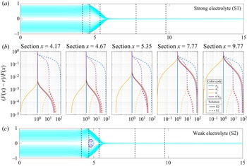
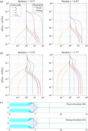
Also, in figures 3 and 4 we have plotted in log scale the profiles of concentration and relative conductivity for several  $x$ sections in the limits of strong electrolyte (solution S1 and S3 plotted with dash line) and weak electrolyte (S2 and S4; continuous line). To obtain a description that is as detailed as possible of the Debye layer, the ordinates reflect the relative radial position from the interface
 $y=1-\eta =(F(x)-r)/F(x)$, which ranges from the vicinity of the interface (or the needle) for
 $y \rightarrow 0$ to the axis of symmetry
 $y = 1$. It is evident from both panels (a) and (b) in figure 2, and from profiles in figures 3 and 4, that the bulk concentrations of the species are far of being uniform in a strong electrolyte and, as a consequence, the bulk conductivity is not homogeneous; the concentrations rapidly grow from the axis of symmetry to the interface. The profiles of concentrations in figure 3 and the matching between contours of cations and relative conductivity in figure 2(b) show that the conductivity is fundamentally determined by the cation due to its larger diffusivity and concentration in positive polarity. This behaviour is not associated with the ion diffusivity as it is observed either when the paired ions are highly mobile and dissimilar (solutions S1 and S2) or slow and of equivalent size (solutions S3 and S4).
(a) The interface shape and streamlines corresponding to solution S1; (b) from left to right, the radial profiles of concentrations  $n_+$,
 $n_-$,
 $n_n$ and
 $\kappa /\kappa _o$ are plotted in log scale for different
 $x$ sections and for operating conditions
 $V_e=4.0 \times 10^{-3}$ (
 $Q/Q_o=10$) and
 $\varPhi = 3.0$. Dashed and continuous lines are for solutions S1 and S2, respectively; (c) interface shape and streamlines corresponding to solution S2. In top and bottom figures the position at which the sections are located are also shown.

The radial profiles of the concentrations  $n_+$,
 $n_-$,
 $n_n$ and
 $\kappa /\kappa _o$, plotted in log scale for different
 $x$ sections and for operating conditions
 $V_e=4.67 \times 10^{-3}$ (
 $Q/Q_o=3.45$) and
 $\varPhi = 3.4$. Dashed and continuous lines for solutions S3 and S4, respectively. Interface shape and streamlines corresponding to both solutions are shown at the bottom of the graph. The position at which the profile sections are located are also shown.

On the contrary, as can be observed in figures 3 and 4, the weak electrolyte solutions S2 and S4 are characterized by flat radial profiles of the concentration of the neutral ion par  $n_n$ in all the sections. The concentrations of anion and cations (and therefore the conductivity) in the bulk are uniform in this case. Naturally, the uniformity disappears in the Debye layer, where the electrical cation–anion migration in opposite directions, limited by the thermal diffusion, produces unmatched concentrations. The ion distributions in weak electrolytes like S2 and S4 are strongly mediated by the uniformity of the concentration of the neutral species, a consequence of the effective re-association reaction.
On the other hand, a strong electrolyte (e.g. solutions S1 and S3) is not determined by the concentration of the neutral ion pair but by the electrostatic boundary condition of continuous electric displacement, (2.8). As a consequence, the concentrations of anions and cations in the bulk do not match. Thus, the conductivity coincides with the average value only in the vicinity of the axis of revolution  $y=1$.
The maximum of  $n^+$ is located at the interface obviously due to the positive voltage applied to the needle, the concentration being of the same order for weak and strong electrolytes since it determines the overall macroscopic EHD balances of the system at the interfaces. In contrast, the interfacial value of
 $n^-$ is strongly dependent of the electrolyte strength, being for weak electrolytes an order of magnitude smaller than for strong electrolytes. As a consequence the net charge contained within the Debye layer, in the weak electrolytes TCJ is larger. Therefore, electrical forces are usually larger and the cone shorter under the same applied voltage, as can be observed comparing top and bottom profiles in figure 3. The width of the Debye layer grows downstream, occupying up to 50 % of the jet radius in sections
 $x=7.77$ and beyond in figure 3 or 20 % in figure 4. In conclusion, the interfacial character of the charge characteristic of the LDM becomes completely questionable in the jet region.
4.1.1. Positive and negative polarities: the large differences
To reveal the contribution of each ionic species to the local conductivity observed, we have focused on the strong and weak electrolyte solutions S1 and S2 characterized by quite different ionic mobilities (table 1). Setting a liquid flow rate such that the dimensionless maximum velocity at the tube entrance is  $V_e=0.004$, we have connected the capillary to positive and negative polarities with electric potential values
 $\varPhi =3.3$ and
 $\varPhi =-3.1$ in the case of the strong solution S1, while both positive and negative voltages are set to the same voltage drop,
 $|\varPhi |=3.1$, for S2.
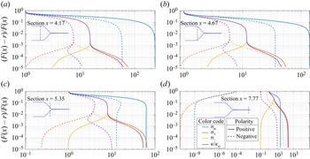
In the case of S1, the slightly different potential needed to have both cone shapes coincident indicates a global difference (approximately 6.4 %) in the relative strengths of the resulting electrical and surface tension forces. However, the most conspicuous difference lies in the radically different profiles of ionic concentrations found for each applied voltage polarity observed in figure 5, which yield total electric currents ejected (i.e. the asymptotic values of  $I_f(x)$ in the jet) equal to
 $I=15.72$ and
 $-$6.00 for positive and negative voltages, respectively. In particular, the near absence of neutral and positive ions in the developed jet, and the completely dominant contribution of negative ions to the conductivity under negative polarity, are remarkable features. In fact, the smaller mobility of the anions (table 1) and the asymptotic absence of cations in the jet are responsible of the large difference in the ejected electric currents. Provided this result is correct, the model could be used to optimize the differential resolution and sensitivity of electrospray mass spectrometry in routine positive and negative ionization modes, for example.
Radial distribution of ionic concentrations and relative conductivity in several sections for positive polarity (continuous lines) and negative polarity (dashed lines). The injected fluid is the strong electrolyte solution S1. Ordinates are relative distances from the surface towards the axis. The cases compared share the same flow rate (dimensionless maximum velocity at the tube entrance  $V_e=0.004$). The applied voltages for both polarities have been adjusted to make the cone-jet shapes coincident (
 $\varPhi =3.3$ and
 $\varPhi =-3.1$). The sections shown are located at
 $x_s =$ 4.17, 4.67, 5.35 and 7.77. The concentration of the salt, (
 $n_n$; blue colour), cation concentration (
 $n_+$; orange colour), anion concentration (
 $n_-$; yellow colour) and relative conductivity cation (
 $\kappa /\kappa _o$; colour purple) are shown in each section.

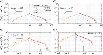
The characteristic radial profiles for a weak electrolyte solution S2 are shown in figure 6. We can observe that the radial distributions of the cation and anion concentrations mirror each other according to the applied voltage in the cone: for  $x=4.17$ and
 $x=4.67$,
 $n^+$ (
 $n^-$) with positive voltage is equal to
 $n^-$ (
 $n^+$) with negative voltage. This perfect symmetry decays beyond the cone-to-jet transition region (see profiles at sections
 $x=5.35$ and
 $x=7.77$ in figure 6). The magnitude of the net charge contained in the Debye layer is, thus, almost independent of the sign of the applied voltage and the shape of the cone jet is independent of the polarity of the voltage drop. However, as the mobilities of the cation and anion are very different, so is the distribution of the conductivity in the Debye layer for the two polarities. Since the average conductivity is higher for the positive polarity, the electric current is more intense:
 $I=7.99$ vs
 $I=-4.72$ for the reverse polarity.
Radial distribution of ionic concentrations and relative conductivity in several sections for positive polarity (continuous lines) and negative polarity (dashed lines). The injected fluid is the weak electrolyte solution S2. Ordinates are relative distances from the surface towards the axis. The cases compared share the same flow rate (dimensionless maximum velocity at the tube entrance  $V_e=0.004$). The applied voltages for both polarities have been adjusted to make the cone-jet shapes coincident (
 $|\varPhi |=3.1$). The sections shown are located at
 $z_s = 4.17$, 4.67, 5.35 and 7.77. The concentration of the salt, (
 $n_n$; blue colour), cation concentration (
 $n_+$; orange colour), anion concentration (
 $n_-$; yellow colour) and relative conductivity cation (
 $\kappa /\kappa _o$; colour purple) are shown in each section.

Although the electrospray literature routinely reports differences according to the voltage polarity (Lozano & Martínez-Sánchez Reference Lozano and Martínez-Sánchez2005; Kim et al. Reference Kim, Teramoto, Negishi, Ogata, Kim, Pongrác, Machala and Gañán-Calvo2014), especially in mass spectrometry (Wang et al. Reference Wang, Hayeck, Brüggemann, Yao, Chen, Zhang, Emmelin, Chen, George and Wang2017), such differences are usually negligible (Wang, Allgeier & Weatherley Reference Wang, Allgeier and Weatherley2021) under operational conditions without gas discharges. In contrast, in the case of a strong electrolyte solution, we observe drastically different ion concentration profiles in the jet for mobility differences that can be readily found in electrospray mass spectrometry, pointing to an obvious hidden inconsistency in the assumptions made with our model (an inconsistency that can be anticipated as the absence of charge adsorption at the interface).
4.2. Discussion
In the first place, the PNP equations under the assumption of negligible ion interface adsorption together with our accurate numerical scheme provide a detailed description of the internal structure of the Debye layer along the whole cone-jet interface. Interestingly, if one observes the lines of constant concentration (figure 2), they are fundamentally normal to the equipotential lines, and also parallel to the streamlines in figures 3 and 4. This occurs even for the case of cone-jet solutions of strong electrolytes (solutions S1 and S3), which according to (2.12) would result in  $\boldsymbol {\nabla } \boldsymbol{\cdot} (\kappa \boldsymbol {E}) \simeq 0$. This is the hallmark of charge relaxation, which is readily assumed in the LDM. Consistently with this, weak electrolytes (e.g. solutions S2 and S4) behave according to expectations based on the LDM approximations, at least in the cone-jet transition region (figure 3) where the electric current and ultimately the cone-jet shape are determined (Gañán-Calvo et al. Reference Gañán-Calvo, López-Herrera, Herrada, Ramos and Montanero2018). However, the dramatic radial variations in conductivity (or cation and anion concentrations) in the liquid bulk outside the Debye layer for strong electrolytes using the PNP are totally inconsistent with the LDM, that assumes a constant bulk conductivity. This inconsistency is even more evident with ion pairs formed by dissimilar ion–cation couples like the solution S1. Hence,
 $\kappa =\textrm {const.}$ (i.e. the LDM) would be a sufficient but not necessary condition for charge relaxation.
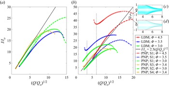
To assess the key differences between the present electrokinetic model with negligible surface ion adsorption and the LDM in terms of their macroscopic consequences in the case of strong electrolyte solutions, we first compare the resulting cone-jet shapes using solution S1 with those obtained with the LDM in figure 7. An immediate observation is the important differences in the elongation of the meniscus that points to a significantly smaller effect of the surface stresses in the case of this PNP model if the electrolyte strength is high. This should be consistent with Mori's simplification assuming that electrical displacements should be continuous across the interface, according to the absence of any surface charge related to interfacial adsorption. The rationale behind that simplification is the theoretical completeness of the full PNP bulk equations that should reflect the entire physics through a strictly conservative volumetric formulation, particularly in the Debye layer. Indeed, numerical schemes that do not rely on an accurate description of the interfaces, but on bulk (volumetric) equations (such as either the PNP approach limited to the set ((2.4)–(2.6)) implemented in López-Herrera et al. (Reference López-Herrera, Gañán-Calvo, Popinet and Herrada2015) or the EHD model outlined at the beginning of § 2.2, used in López-Herrera et al. Reference López-Herrera, Popinet and Herrada2011) have provided excellent results in both steady TCJ (Herrada et al. Reference Herrada, Lopez-Herrera, Gañan-Calvo, Vega, Montanero and Popinet2012) and unsteady ejection (Gañán-Calvo et al. Reference Gañán-Calvo, López-Herrera, Rebollo-Muñoz and Montanero2016). A critical point in defence of volumetric formulations tackled via volumetric numerical approaches like the VoF schemes (e.g. Basilisk ) is that the Debye layer is subsumed in the discrete volume cells around the interface. Hence, the integral contribution of the Debye layer to the global charge balance is consistently solved according to the volumetric charge conservation principle. However, when an extremely detailed scheme is applied to resolve that layer using the same scheme, the global picture can be drastically altered. A further illustration on the dramatic differences between an electrokinetic formulation in the absence interfacial adsorption and the LDM when both are applied to electrospray is given in figure 8(b), where the relative flow rate  $Q/Q_o$ is used as a free parameter covering two orders of magnitude from
 $Q/Q_o \sim O(1)$ to approximately
 $4 \times 10^2$.
Profiles of the cone-jet configurations for two liquid flow rates and three applied voltages, using both solution S1 and LDM models. (a) and (b) panels correspond to  $V_e =1.74 \times 10^{-2} (Q/Q_o=43.5)$ and
 $V_e =4.0 \times 10^{-3} (Q/Q_o=10)$, respectively.

Electric current  $I/I_o$ as a function of
 $(Q/Q_o)^{1/2}$ for three applied voltages, according to both PNP and LDM models. (a) Results obtained with the PNP equation applied to the weak electrolyte solutions S2 (
 $\varPhi = 3.0$) and S4 (
 $\varPhi = 3.4$); the LDM results with
 $\varPhi = 3.0$ and 3.5 are also shown. (b) Results for strong electrolytes S1 (
 $\varPhi = 3.0$, 3.5 and 4.5) and S3 (
 $\varPhi = 3.4$); the LDM results with
 $\varPhi = 3.0$, 3.5 and 4.5 are also shown. Vertical lines in panel (b) indicate de
 $(Q/Q_o)^{1/2}$ values corresponding to the profiles shown in figure 3. The black continuous lines indicate the scaling law of Gañán-Calvo et al. (Reference Gañán-Calvo, Barrero and Pantano1993). Note that the scaling law based on the LDM gives
 $r_j=0.67(Q/Q_o)^{1/2} d_o=0.16$ mm (Gañán-Calvo Reference Gañán-Calvo1999), while the profile using the LDM model gives
 $r_j=0.18$ mm at the right end of the jet in the figure.

The degree of agreement of the models with experimentally verified scaling laws is conditioned by the geometry of the cone jet (Gañán-Calvo et al. Reference Gañán-Calvo, López-Herrera, Herrada, Ramos and Montanero2018). The standard TCJ configuration implies the existence of a quasi-electrohydrostatic region; the quasi-static meniscus held by the basic balance of electrostatic Maxwell stresses and surface tension for a given set of boundary conditions and applied voltage (Pantano, Gañán-Calvo & Barrero Reference Pantano, Gañán-Calvo and Barrero1994). The smaller the jet radius compared with the tube radius, the larger the quasi-electrohydrostatic region and the closer the agreement with those scaling laws. A simple way to assess the jet-to-tube scale ratio is to introduce the characteristic EHD length  $d_o=({\sigma \varepsilon _o^2}/{\rho \kappa ^2})^{1/3}$ (Gañán-Calvo Reference Gañán-Calvo1999). In the case shown in figure 2 (solution S1;
 $Q/Q_o = 10$;
 $\varPhi = 3.0$),
 $d_o=11.6\ \mathrm {\mu }$m, and
 $(R_n/d_o)^{-1}=1.16 \times 10^{-2}$, which yields relatively large jet diameters compared with usual TCJ standards, where
 $(R_n/d_o)^{-1}$ is usually smaller than approximately
 $10^{-3}$. For example, for
 $(Q/Q_o)^{1/2}=10$, one would have a predicted jet radius
 $r_j\simeq 0.67 (Q/Q_o)^{1/2} d_o$ (Gañán-Calvo Reference Gañán-Calvo1999), of the order of 0.08 mm, according to the scaling laws. Thus, the profiles may deviate significantly from a canonical TCJ configuration in this study due to the existence of a quite large cone-jet transition region, as can be seen in figure 8 for
 $(Q/Q_o)^{1/2}\simeq 20$ for the PNP (panel c) and the LDM models (panel d). Again, one can observe that the acceleration of the liquid is significantly smaller for the PNP formulation compared with the LDM model, consistently with a reduced tangential stress on the liquid in the former due to the absence of surface charge.
Finally, it is noticeable that, while for the large  $Q/Q_o$ values our results deviate from the scaling law, which would be expected from the large jet diameters compared with
 $R_n$, the results of the LDM comply with the scaling law by Gañán-Calvo et al. (Reference Gañán-Calvo, Barrero and Pantano1993) for the emitted electric current
 $I/I_o$ (see the inset of figure 8) as
 $Q/Q_o$ is reduced. This scaling law was also discussed in Gañán-Calvo (Reference Gañán-Calvo1999); Hartman et al. (Reference Hartman, Brunner, Camelot, Marijnissen and Scarlett1999) and Gañán-Calvo (Reference Gañán-Calvo2004) with slightly different prefactors. This consistency is particularly remarkable in figure 8(a) when using the present electrokinetic model for weak electrolytes. Here, the prefactor 2.47 used in the plot (black continuous line) was that anticipated by Gañán-Calvo et al. (Reference Gañán-Calvo, Barrero and Pantano1993) from early experiments using different liquid formulations: note that both S2 and S4 remarkably converge to that scaling law and prefactor (quite insensitive to the voltages applied in the range explored). In effect, the speed and efficiency of the association reaction for weak electrolytes is sufficient to homogenize the conductivity within the Taylor cone bulk, a hallmark of the LDM despite the intense applied voltage – well above the thermal one.
However, for strong electrolytes (panel b), the differences between present electrokinetic and LDM models become extreme. In fact, while the LDM scheme approaches the scaling law as  $Q/Q_o$ is reduced, characterized by the weak influence of the applied voltage on the total current, the PNP approach strongly departs from that. Hence, given that the TCJ scaling laws assume
 $\kappa =\textrm {const.}$, and those laws have been verified for this flow rate range (Gañán-Calvo et al. Reference Gañán-Calvo, Barrero and Pantano1993, Reference Gañán-Calvo, López-Herrera, Herrada, Ramos and Montanero2018), our results indicate that the hypothesis of Mori & Young (Reference Mori and Young2018) neglecting surface charge absorption would not be applicable for TCJ electrosprays of strong electrolytes, which is indeed consistent with the restriction of those authors to weak electrolytes.
From this study, one may conclude that a fundamental feature would be needed to extend the validity of the Mori & Young approach to the electrospray of fully dissociated solutions. In particular, the drastic inhomogeneity of the electric current yielded by a electrokinetic formulation without surface charge due to ion interface adsorption may lead to an intrinsically unstable and therefore unphysical state. In other words, the imposition of zero surface charge in steady TCJ models using the PNP equations that accurately resolve the Debye layer could be a strong artificial requirement, leading to an unphysical (or unstable) state characterized by an inhomogeneous electric bulk conductivity. Our best guess is that the PNP equations should be completed with some degree of ion interface adsorption obeying a strictly interfacial charge conservation equation (an augmented version of the one used in the LDM model). In this way, a non-zero surface charge as the one suggested by Schnitzer & Yariv (Reference Schnitzer and Yariv2015) should be incorporated in the model for a complete formulation of general EHD problems, at least for completely dissociated solutions.
Acknowledgements
The authors would like to acknowledge the reviewers for their contributions, which greatly improved the paper.
Funding
This work was supported by the program “Proyectos I+D+i FEDER Andalucía 2014-2020” (project US-1380775) and the Ministerio de Ciencia e Innovación of the Kingdom of Spain (project PID2019-108278RB-C31).
Declaration of interests
The authors report no conflict of interest.
Author contributions
J.L.-H. performed the simulations. J.L.-H. and M.A.H. developed the numerical code. J.L.-H. and A.M.G.-C. wrote the paper. All authors contributed equally to analysing data and reaching conclusions.












 Open access

