1 Introduction
Turbulence in the atmospheric boundary layer is responsible for the dispersion of pollutants, dust, sand and other constituents (Garratt Reference Garratt1994). However, even with dilute volume concentrations, turbulence modulation by particles still poses a formidable challenge to fully understanding how these constituents alter their own transport (Balachandar & Eaton Reference Balachandar and Eaton2010). Turbulence in the atmospheric boundary layer is characterized by very high Reynolds numbers, and is therefore subject to the numerous interactions between inner and outer layers, including the dynamics of the so-called very-large-scale motions which develop (Smits, McKeon & Marusic Reference Smits, McKeon and Marusic2011; Inoue et al. Reference Inoue, Mathis, Marusic and Pullin2012; Jiménez Reference Jiménez2018). Since in many atmospheric multiphase flows the dispersed phase is emitted from a surface (e.g. sand saltation, bubbles bursting at a water surface), the effect of particulates on inner–outer interactions and more specifically on the regeneration cycles of near-wall coherent motions is the primary interest of the present study. While the complexity of high-Reynolds-number, multiphase, turbulent flows is high due in large part to the wide range of relevant spatial and temporal scales, the present aim is to simplify the problem and examine one key aspect of the larger picture: the regeneration cycle of coherent structures in the overlap region of wall-bounded turbulence. In this regard, turbulent plane Couette flow (PCF) at low Reynolds number is known to contain the self-sustained processes exhibited by turbulent coherent structures (Hamilton, Kim & Waleffe Reference Hamilton, Kim and Waleffe1995; Waleffe Reference Waleffe1997), as well as large-scale structures interacting with smaller near-wall motions (Komminaho, Lundbladh & Johansson Reference Komminaho, Lundbladh and Johansson1996; Kitoh, Nakabyashi & Nishimura Reference Kitoh, Nakabyashi and Nishimura2005). This set-up is therefore a representative, computationally inexpensive candidate for shedding light on particle transport and the fundamental modification of the regeneration cycle and inner/outer interactions.
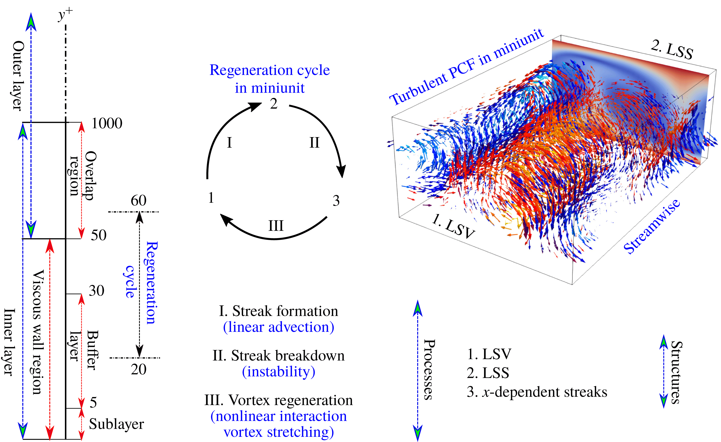
Sketch of various wall regions and boundary layers in wall units (Jiménez & Pinelli Reference Jiménez and Pinelli1999; Pope Reference Pope2000) and the regeneration cycle sub-steps (Hamilton et al. Reference Hamilton, Kim and Waleffe1995; Waleffe Reference Waleffe1997; Schoppa & Hussain Reference Schoppa and Hussain2002) in a domain size called ‘minimal’ unit. In the top-right is the flow field in turbulent PCF in miniunit. Large-scale vortex (LSV) is shown by vector fields and coloured by the streamwise vorticity. Large-scale streak (LSS) is shown by the contour of the streamwise velocity magnitude.

It is commonly accepted that the full regeneration cycle in the inner layer exhibits the main characteristics of turbulence (Hamilton et al.
Reference Hamilton, Kim and Waleffe1995; Waleffe Reference Waleffe1997; Jiménez & Pinelli Reference Jiménez and Pinelli1999; Kawahara & Kida Reference Kawahara and Kida2001; Schoppa & Hussain Reference Schoppa and Hussain2002). Figure 1 provides a schematic of the various regions near the wall, as well as the key turbulent structures and processes which make up the regeneration cycle in the region of
 $20<y^{+}<60$
; see Waleffe (Reference Waleffe1997) and Jiménez & Pinelli (Reference Jiménez and Pinelli1999). This self-sustained regeneration cycle is marked by three important structures: large-scale vortices (LSVs), large-scale streaks (LSSs) and
 $x$
-dependent meandering streaks; each stage of the regeneration process is associated with sequential sub-processes. Specifically, the streaks are generated by a linear process, the so-called lift-up effect, whereas the following two processes are the result of nonlinear interactions called streak breakdown and vortex regeneration. The regeneration cycle was first investigated by Hamilton et al. (Reference Hamilton, Kim and Waleffe1995) in PCF using a so-called ‘miniunit’ configuration, which is the minimal geometric domain that is sufficient to accommodate the self-sustained flow structures for single-phase turbulence. This minimal simulation domain was carefully examined in Couette flow configuration by Hamilton et al. (Reference Hamilton, Kim and Waleffe1995) and pressure-driven flow by Jiménez & Moin (Reference Jiménez and Moin1991). In both cases, the spanwise length is slightly larger than
 $100$
wall units, which corresponds to the spanwise characteristic spacing between two coherent structures.
The modulation of the regeneration cycle has been found to be related to the spatial distribution of a particulate phase. In fully resolved simulations with finite-sized, neutrally buoyant particles, the cycle is promoted in turbulent pressure-driven flow, and is hardly modified in turbulent PCF (Brandt Reference Brandt2014; Wang, Abbas & Climent Reference Wang, Abbas and Climent2018). In the case of PCF, particles are more likely to be present in the core of the large-scale rolls which are mainly responsible for dissipating energy. The same phenomenon is also observed experimentally in Taylor–Couette flow (Majji, Banerjee & Morris Reference Majji, Banerjee and Morris2018) if the particle concentration is low and and the particles are relatively small compared with the gap. However, in pressure-driven flow, finite-size neutrally buoyant particles show a non-monotonic effect on laminar-to-turbulent transition. From an experiment of particle-laden, pressure-driven pipe flow, Matas, Morris & Guazzelli (Reference Matas, Morris and Guazzelli2003) found that low volume concentrations (less than
 $20\,\%$
) of large particles (particle to pipe diameter ratio of around
 $1/20$
) sustain the turbulent state and decrease the transition threshold, whereas a high concentration of small particles advances the transition threshold significantly. Wang et al. (Reference Wang, Abbas and Climent2018) further found that particles tend to trigger instability in pressure-driven flow due to the particles’ preferential presence in near-wall streaks.
In general, turbulence modulation is found to depend on the size ratio between the particle and turbulence length scales, and on the time scale ratio between the particle response time with a characteristic time scale of the flow – i.e. the dimensionless Stokes number
 $St$
(Gore & Crowe Reference Gore and Crowe1989; Elghobashi Reference Elghobashi1994). Gore & Crowe (Reference Gore and Crowe1989), for instance, proposed a relationship of size ratio between particle diameter and the flow integral length scale to flow turbulent intensity attenuation/augmentation. Tanaka & Eaton (Reference Tanaka and Eaton2008) formulated a dimensionless particle momentum number to predict turbulence modulation which includes the flow microscale (Kolmogorov scale), the energy-containing scale, as well as the Stokes number. At high Reynolds number, Tanaka & Eaton (Reference Tanaka and Eaton2008) divided the turbulent modification into three regions: moderate momentum number tends to attenuate the turbulence whereas low or high momentum number tend to augment the turbulence. For heavy particles which can be reasonably modelled using only a drag force (i.e. neglecting lift, added mass and Basset history terms; see Maxey & Riley (Reference Maxey and Riley1983)), Balachandar & Eaton (Reference Balachandar and Eaton2010) proposed that the turbulence modulation mechanisms can be simplified: turbulence reduction comes from enhanced inertia and increased dissipation arising from particle drag, whereas the turbulence enhancement is due to enhanced velocity fluctuation from wake dynamics. A large body of work on turbulent kinetic energy modification (Squires & Eaton Reference Squires and Eaton1990; Elghobashi & Truesdell Reference Elghobashi and Truesdell1993; Pan & Banerjee Reference Pan and Banerjee1996; Burton & Eaton Reference Burton and Eaton2005), interphasial energy transfer (Zhao, Andersson & Gillissen Reference Zhao, Andersson and Gillissen2013), particle transfer and segregation (Marchioli & Soldati Reference Marchioli and Soldati2002) or drag reduction (Li et al.
Reference Li, McLaughlin, Kontomaris and Portela2001; Dritselis & Vlachos Reference Dritselis and Vlachos2008) can be found in the literature.
While we are ultimately interested in the modulation of high-Reynolds-number wall turbulence due to inertial particles, our specific focus in this work is on the modification of the near-wall regeneration cycle and its close connection with laminar-to-turbulent transition as a model for inner–outer interactions; this influence of a dispersed phase in turbulent flows has received relatively little attention. At Reynolds numbers close to the onset of transition, Klinkenberg, De Lange & Brandt (Reference Klinkenberg, De Lange and Brandt2011) proposed a stability Stokes number, where at small values (fine particles) the critical Reynolds number decreases proportionally to the particle mass fraction, and where at intermediate values yields an increase of the critical Reynolds number, the enhancement is proportional to the volume fraction. Through linear analysis of the Orr–Sommerfeld equation coupled to a dispersed phase via drag, Saffman (Reference Saffman1962) theoretically predicted that fine particles tend to destabilize the gas flow whereas coarse particles have a stabilizing action. The drag coupling between phases therefore has competing effects: low-inertia particles tend to destabilize the flow by adding to the effective density of the gas, and high-inertia particles tend to act as an extra dissipation source, thereby stabilizing the flow. Following the formulation proposed by Saffman (Reference Saffman1962), Michael (Reference Michael1964), Rudyak, Isakov & Bord (Reference Rudyak, Isakov and Bord1997) and Klinkenberg et al. (Reference Klinkenberg, De Lange and Brandt2011) numerically solved the modified Orr–Sommerfeld equation for plane Poiseuille flow. Michael (Reference Michael1964) showed an increased critical Reynolds number at low particle concentration whereas Rudyak et al. (Reference Rudyak, Isakov and Bord1997) and Klinkenberg et al. (Reference Klinkenberg, De Lange and Brandt2011) found that the critical Reynolds number reaches a maximum and then decreases gradually with increasing particle relaxation time.
Other configurations have also been theoretically predicted: Dimas & Kiger (Reference Dimas and Kiger1998) studied a particle-laden mixing layer and DeSpirito & Wang (Reference DeSpirito and Wang2001) analysed a particle-laden jet. A similar conclusion is drawn that small, low-inertia particles induce a destabilization effect whereas large-Stokes-number particles stabilize, and that the effect is approximately proportional to the particle mass loading (at least in dilute concentrations). For these stability analyses, however, the particles often must be assumed to be homogeneously distributed or distributed with an assumed profile; nonlinear effects such as particle preferential accumulation and the dynamics of the near-wall regeneration cycles are difficult to include in the analysis. Some nonlinear studies on transition do exist, including those of Klinkenberg et al. (Reference Klinkenberg, De Lange and Brandt2011, Reference Klinkenberg, Sardina, De Lange and Brandt2013), who also find that small inertia tends to decrease the critical Reynolds number whereas particles with intermediate Stokes numbers increase the critical Reynolds number. From dilute limit to high mass loading, Capecelatro, Desjardins & Fox (Reference Capecelatro, Desjardins and Fox2018) find that fluid-phase turbulence kinetic energy is generated by mean-shear production in dilute limit (
 $\overline{\unicode[STIX]{x1D6F7}_{m}}\leqslant 1$
), whereas it is entirely generated by drag production at high mass loading (
 $\overline{\unicode[STIX]{x1D6F7}_{m}}\geqslant 10$
). In the intermediate regime (
 $2\leqslant \overline{\unicode[STIX]{x1D6F7}_{m}}\leqslant 4$
), the flow relaminarizes due to higher rate of dissipation compared to production of turbulence kinetic energy. Mechanisms regarding the disruption of turbulence regeneration, however, are still an open question.
To study the particle-induced modulation of the self-sustained regeneration cycle in wall turbulence, numerical simulations are performed for particle suspensions in PCF in a ‘miniunit’ domain. In previous work, finite-size particles with low Stokes number are found to hardly modify the regeneration cycle due to particles preferentially accumulating in the LSVs (Wang et al. Reference Wang, Abbas and Climent2018). At a higher Reynolds number, however, pointwise inertial particles with moderate to high Stokes numbers preferentially ‘operate’ on flow structure scales associated with the particle response time scale (Richter & Sullivan Reference Richter and Sullivan2013, Reference Richter and Sullivan2014; Richter Reference Richter2015), but this effect on the regeneration cycle remains unclear. While these previous simulations of particle-laden turbulent flows have identified numerous modifications to the flow statistics, energy spectra and coherent structures, the dynamical processes behind these modifications have not been analysed in detail. Therefore a primary purpose of this work is to link our existing knowledge of particle-laden turbulence modification with the flow dynamics via modifications to the near-wall regeneration cycle. In this paper, § 2 presents the numerical method, the flow configuration and parameter choices. Particle inertial effects on transition are presented in § 3. The modulation of the turbulence regeneration cycle is reported through modal analysis in § 4.
2 Simulation method and validation
2.1 Numerical method
Direct numerical simulations of single-phase flows are performed for an incompressible Newtonian fluid. A pseudospectral method is employed in the periodic directions (streamwise,
 $x$
, and spanwise,
 $z$
) and second-order finite differences are used for spatial discretization in wall-normal
 $y$
direction. The solution is advanced in time by a third-order Runge–Kutta scheme. Incompressibility is achieved by correcting the pressure contribution, which is a solution of a Poisson equation. The fluid velocity and pressure fields are a solution of the continuity equation (2.1) and momentum balance equations (2.2) and (2.3):
 $$\begin{eqnarray}\displaystyle & \displaystyle \frac{\unicode[STIX]{x2202}u_{j}}{\unicode[STIX]{x2202}x_{j}}=0, & \displaystyle\end{eqnarray}$$
 $$\begin{eqnarray}\displaystyle & \displaystyle \frac{\unicode[STIX]{x2202}u_{i}}{\unicode[STIX]{x2202}t}+u_{j}\frac{\unicode[STIX]{x2202}u_{i}}{\unicode[STIX]{x2202}x_{j}}=-\frac{1}{\unicode[STIX]{x1D70C}_{f}}\frac{\unicode[STIX]{x2202}p}{\unicode[STIX]{x2202}x_{i}}+\unicode[STIX]{x1D708}\frac{\unicode[STIX]{x2202}u_{i}}{\unicode[STIX]{x2202}x_{j}\unicode[STIX]{x2202}x_{j}}+\frac{1}{\unicode[STIX]{x1D70C}_{f}}F_{i}, & \displaystyle\end{eqnarray}$$
 $$\begin{eqnarray}\displaystyle & \displaystyle F_{i}^{k}=-\mathop{\sum }_{k_{s}=1}^{8}\mathop{\sum }_{n=1}^{N_{k_{s}}}\frac{w_{k_{s}}^{n}}{\triangle V_{k_{s}}}f_{i}^{n}. & \displaystyle\end{eqnarray}$$
Using a projection technique, the body force in the momentum balance equation (2.3) accounts for the particle momentum contribution to node
 $k$
of the fluid based on particles in all of the eight computational volumes (
 $k_{s}$
) which share this node. Parameter
 $w_{k_{s}}^{n}$
is the linear geometric weight for each particle
 $n$
based on its distance from node
 $k$
, and the inner summation is over all
 $N_{k_{s}}$
particles in the volume
 $k_{s}$
.
Numerical simulations of particle trajectories and suspension flow dynamics are based on the standard Lagrangian point-particle approximation where the particle-to-fluid density ratio
 $r\equiv \unicode[STIX]{x1D70C}_{p}/\unicode[STIX]{x1D70C}_{f}\gg 1$
and the particle size is smaller than the smallest viscous dissipation scales of the turbulence. As a consequence of this and the low volume concentrations (a maximum volume fraction of
 $\overline{\unicode[STIX]{x1D6F7}_{V}}$
less than
 $1\times 10^{-3}$
is used in this study), only the Stokes drag force and two-way coupling have been incorporated (see Balachandar & Eaton Reference Balachandar and Eaton2010). The velocity of particle
 $n$
is governed in (2.4) and particle trajectories are then obtained from numerical integration of the equation of motion (2.5):
 $$\begin{eqnarray}\displaystyle & \displaystyle \frac{\text{d}u_{p,i}^{n}}{\text{d}t}=\frac{f_{i}^{n}}{m_{p}}=\frac{1}{\unicode[STIX]{x1D70F}_{p}}[1+0.15(Re_{p}^{n})^{0.687}](u_{f,i}^{n}-u_{p,i}^{n}), & \displaystyle\end{eqnarray}$$
 $$\begin{eqnarray}\displaystyle & \displaystyle \frac{\text{d}x_{i}^{n}}{\text{d}t}=u_{p,i}^{n}, & \displaystyle\end{eqnarray}$$
where
 $\unicode[STIX]{x1D70F}_{p}=\unicode[STIX]{x1D70C}_{p}{d_{p}}^{2}/18\unicode[STIX]{x1D707}$
is the Stokes relaxation time of the particle,
 $m_{p}$
is the particle mass and the particle Reynolds number
 $Re_{p}^{n}=|u_{f,i}^{n}-u_{p,i}^{n}|d_{p}^{n}/\unicode[STIX]{x1D708}$
is based on the magnitude of the particle slip velocity
 $(u_{f,i}^{n}-u_{p,i}^{n})$
and particle diameter
 $d_{p}^{n}$
. In this work, the average
 $Re_{p}^{n}$
is between
 $0.125$
(
 $r=80$
, two-way) and
 $3.25$
(
 $r=8000$
, one-way), which is far smaller than the suggested maximum
 $Re_{p}\approx 800$
for the Stokes drag correction in (2.4) (Schiller Reference Schiller1933). Thus the
 $Re_{p}$
correction to the Stokes drag is minimal in this study. In order to highlight the effect of particle response time, we do not consider gravitational settling. Other terms in the particle momentum equation (see Maxey & Riley Reference Maxey and Riley1983) are neglected since they remain small compared with drag when the density ratio
 $r\gg 1$
. These neglected terms are also found to have less effect on the stability analysis in relatively low-Reynolds-number turbulence as demonstrated by Klinkenberg, de Lange & Brandt (Reference Klinkenberg, de Lange and Brandt2014). Particle–particle collisions are not taken into consideration due to the low volume concentrations, and we exert a purely elastic collision between particles and the upper/lower walls. This purely elastic wall collision is commonly used in gas–solid turbulence (Li et al.
Reference Li, McLaughlin, Kontomaris and Portela2001; Sardina et al.
Reference Sardina, Schlatter, Brandt, Picano and Casciola2012; Zhao et al.
Reference Zhao, Andersson and Gillissen2013). However, we have tested the restitution coefficient
 $|u_{p,init}^{n}/u_{p,final}^{n}|$
between
 $0.5$
and
 $1$
and do not observe significant changes to particle distributions or two-way coupling, consistent with Li et al. (Reference Li, McLaughlin, Kontomaris and Portela2001).
In addition to the point force approximation as implemented in (2.3), there are other techniques that can be used to account for two-way coupling in particle-laden flows. For example Pan & Banerjee (Reference Pan and Banerjee1996) use the pressure gradient and stress tensor from an analytic velocity disturbance field to replace the point force, Capecelatro & Desjardins (Reference Capecelatro and Desjardins2013) use a volume filtering operator to replace the point sources by smoother, locally filtered fields and Gualtieri et al. (Reference Gualtieri, Picano, Sardina and Casciola2015) present an exact regularized point particle method which includes the far-field disturbance by applying a multipole expansion to obtain the Stokeslet. In order to validate our current method, we compared both with the results of Zhao et al. (Reference Zhao, Andersson and Gillissen2013) at
 $Re_{\unicode[STIX]{x03C4}}=180$
with
 $\unicode[STIX]{x03C4}_{p}^{+}=30$
as well as with results from Capecelatro & Desjardins (Reference Capecelatro and Desjardins2013) at
 $Re_{\unicode[STIX]{x03C4}}=235$
with
 $\unicode[STIX]{x03C4}_{p}^{+}=65$
. The mean velocity profile, concentration profile and root mean square (RMS) velocity profile agree well with each other (not shown here), which suggests that the current particle in cell method for two-way coupling is suitable for our study, and is not sensitive to the two-way coupling scheme. Additional details and validation of the numerical scheme can be found in previous work for both one-way coupling and two-way coupling (Richter & Sullivan Reference Richter and Sullivan2013; Sweet, Richter & Thain Reference Sweet, Richter and Thain2018).
2.2 Single-phase PCF
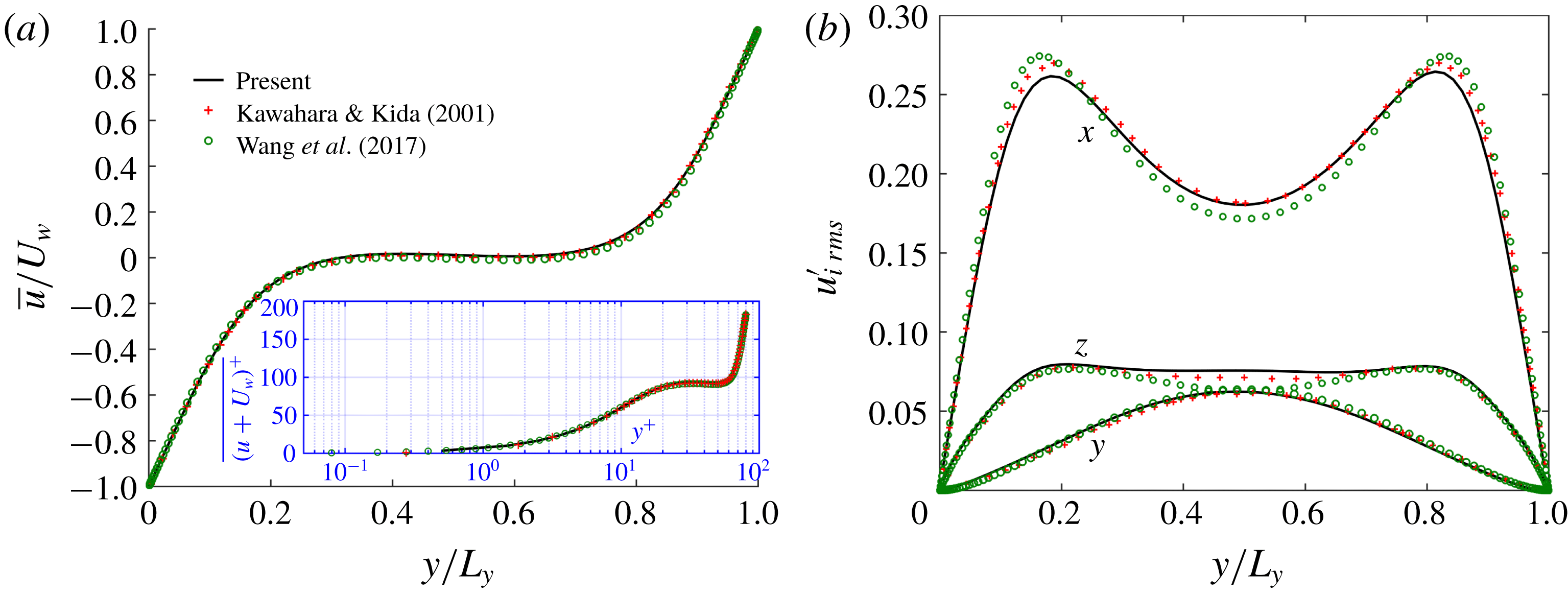
Comparison between current study and published data from Kawahara & Kida (Reference Kawahara and Kida2001) and Wang, Abbas & Climent (Reference Wang, Abbas and Climent2017) in single-phase flow at
 $Re_{b}=400$
: (a) mean velocity profiles; (b) fluctuation velocity RMS in three directions.

Simulation of PCF turbulence in the miniunit configuration is used in the rest of this paper, at a relatively low Reynolds number (just above the onset of transition to turbulence). The flow is driven by two walls moving at equal and opposite velocities, and by imposing a no-slip condition on each. Boundary conditions in the lateral, wall-parallel directions are periodic. The Reynolds number is defined using half of the relative wall velocity and half of the gap between the two walls. The turbulent state is obtained by inducing fluctuations into a laminar flow at a high Reynolds number and once a turbulent state is developed, the Reynolds number is decreased gradually to a desired Reynolds number. The grid used in this work is
 $N_{x}\times N_{y}\times N_{z}=32\times 64\times 32$
(grid convergence tests (not shown here) have ensured that results are independent of grid resolution) corresponding to a resolution in wall units of
 $\unicode[STIX]{x0394}x^{+}\times \unicode[STIX]{x0394}y^{+}$
(wall, centre)
 $\times \unicode[STIX]{x0394}z^{+}\approx 6.8\times (1,1.5)\times 4.7$
. Figure 2 shows the mean velocity profile and velocity fluctuations in all three directions, in comparison with Wang et al. (Reference Wang, Abbas and Climent2017) who used a second-order centred finite volume method and Kawahara & Kida (Reference Kawahara and Kida2001) who used a pseudospectral discretization in all three directions. We can see that the RMS velocity fluctuations from the present simulations agree well with Kawahara & Kida (Reference Kawahara and Kida2001), whereas there is a small discrepancy between the current work and Wang et al. (Reference Wang, Abbas and Climent2017) in the streamwise and spanwise directions near the centre region. This might be due to the slight difference of domain size in the spanwise direction which confines the shape of two counter-rotating rolls in miniunit.
2.3 Suspension flow configurations
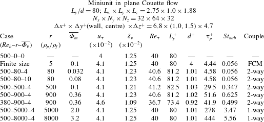
Parameters of baseline numerical simulations. The Reynolds number
 $Re_{b}\equiv U_{w}h/\unicode[STIX]{x1D708}$
, where
 $U_{w}$
is half of the relative velocity and
 $h=L_{y}/2$
is half of the gap between two walls. The friction Reynolds number is
 $Re_{\unicode[STIX]{x1D70F}}\equiv u_{\unicode[STIX]{x03C4}}h/\unicode[STIX]{x1D708}$
and the particle Stokes relaxation time is
 $\unicode[STIX]{x03C4}_{p}\equiv \unicode[STIX]{x1D70C}_{p}d^{2}/(18\unicode[STIX]{x1D70C}_{f}\unicode[STIX]{x1D708})$
, where
 $d$
represents the particle diameter. The superscript ‘
 $+$
’ is the dimensionless number based on viscous scale, where
 $\unicode[STIX]{x1D6FF}_{\unicode[STIX]{x1D708}}$
,
 $u_{\unicode[STIX]{x03C4}}$
and
 $\unicode[STIX]{x1D708}/u_{\unicode[STIX]{x03C4}}^{2}$
correspond to the viscous length scale, velocity scale and time scale, respectively. FCM (force coupling method) is a low-order multipole expansion for capturing finite-size effects used by Wang et al. (Reference Wang, Abbas and Climent2017).

Table 1 contains several selected parameters for the statistical and modal analysis in this study (i.e. the cases used for all analyses but not including the transition tests of § 3.1). The case number indicates the bulk Reynolds number, density ratio and particle volumetric concentration used in that particular simulation. Turbulence–laminar transition occurs near case 380–900–4. Hamilton & Abernathy (Reference Hamilton and Abernathy1994) found a minimum threshold of streamwise vorticity circulation of the LSVs (below which the transition happens), and therefore we use this case to check if this threshold is modified by the presence of inertial particles.
The Kolmogorov scale is difficult to determine and somewhat ambiguous at the low turbulence levels in these simulations, although we can estimate that the minimum dissipation scale is about
 $1.5$
times the viscous length scale at the wall, which itself is about
 $2.0$
times the viscous length scale in the centre (Pope Reference Pope2000). The ratio of the particle to fluid time scale defines the Stokes number
 $St_{turb}\equiv \unicode[STIX]{x03C4}_{p}/\unicode[STIX]{x03C4}_{f}$
, where
 $\unicode[STIX]{x03C4}_{f}\equiv L_{y}/\max (v^{\prime }|w^{\prime })$
is related to the turnover time scale of the LSVs (Massot Reference Massot2007; Wang et al.
Reference Wang, Abbas and Climent2017). The estimation of
 $\unicode[STIX]{x03C4}_{f}$
is about
 $25$
time units (time unit defined as
 $h/U_{w}$
) from figure 7(a). In the context of high-Reynolds-number atmospheric boundary layer flows, the particle Stokes number
 $\unicode[STIX]{x03C4}_{p}^{+}$
based on the viscous scale corresponds to a diameter of
 $d\approx 30~\unicode[STIX]{x03BC}\text{m}$
to
 $d\approx 90~\unicode[STIX]{x03BC}\text{m}$
at
 $Re_{\unicode[STIX]{x03C4}}\approx 10^{4}$
within
 $1$
m of the surface when the particle density is of the order of
 $1000~\text{kg}~\text{m}^{-3}$
. In order to gain insight into the finite-size effects on particle dispersion and turbulence modulation, we specifically select one group of parameters
 $\unicode[STIX]{x03C4}_{p}^{+}$
and
 $St_{turb}$
to be nearly the same as the finite-size particles used in Wang et al. (Reference Wang, Abbas and Climent2017). There are two cases, 500–5000–4 and 500–8000–4, with extremely high density ratios that are intended to help build a complete understanding of the effect of Stokes number on particle dispersion in the LSVs in our model flow. These high density ratios are simulated with one-way coupling only since they fully laminarize the flow at
 $Re_{b}=500$
.
3 Effect of inertial particle response time
3.1 Effects of particle response time and mass loading on transition
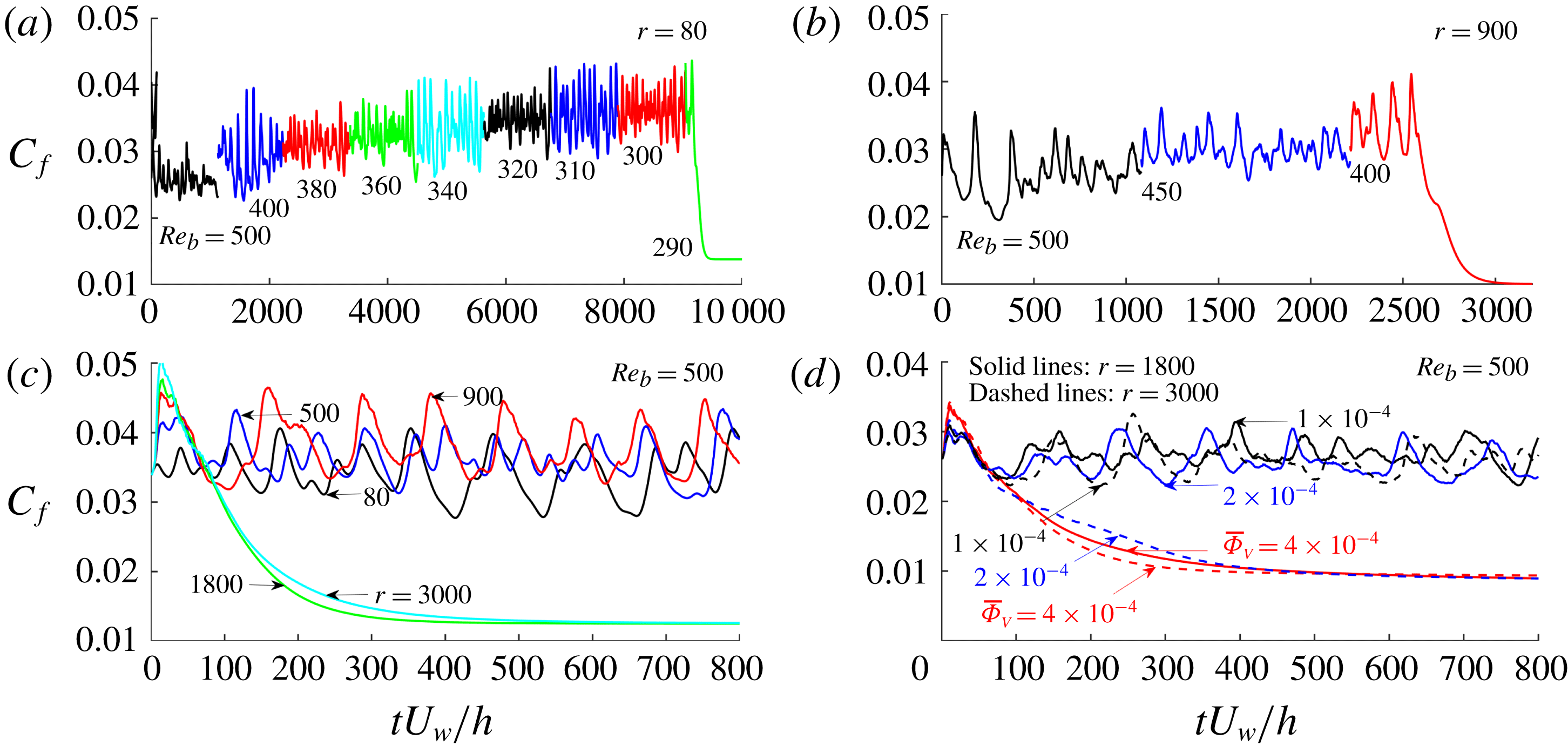
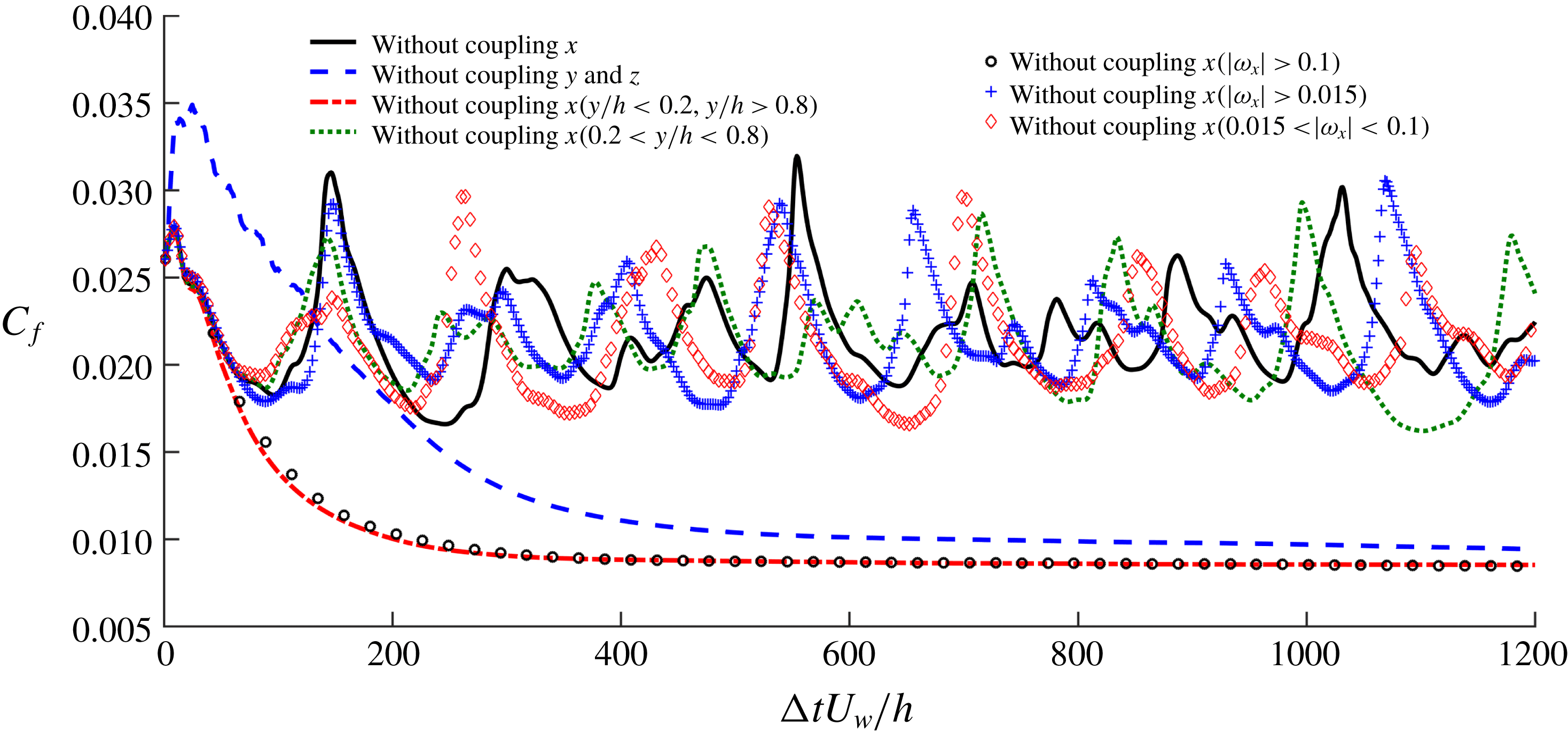
Effect of inertial particles on the turbulence-to-laminar transition as indicated by the temporal evolution of
 $C_{f}$
. This is demonstrated by gradually decreasing
 $Re_{b}$
, density ratio (
 $r$
) and bulk volumetric concentration (
 $\overline{\unicode[STIX]{x1D6F7}_{V}}$
) starting from a fully turbulent simulation at
 $Re_{b}=500$
. (a) Case 500–80–4, decreasing
 $Re_{b}=500$
to
 $Re_{b}=290$
; (b) case 500–900–4, decreasing
 $Re_{b}=500$
to
 $Re_{b}=400$
; (c) fixed
 $Re_{b}=500$
and increasing density ratio
 $r=80$
to
 $r=3000$
; (d) fixed
 $Re_{b}=500$
and two density ratios
 $r=1800$
and
 $r=3000$
,
 $\unicode[STIX]{x1D6F7}_{b}$
decreasing from
 $4\times 10^{-4}$
to
 $1\times 10^{-4}$
.

While linear stability analysis is a key tool in understanding the effects of a dispersed phase on transition, it often must assume that the flow is uniformly (or with some other specified distribution) laden with particles, and that the flow is two-dimensional (Saffman Reference Saffman1962; Michael Reference Michael1964; Dimas & Kiger Reference Dimas and Kiger1998; Rudyak, Isakov & Bord Reference Rudyak, Isakov and Bord1998). Clearly, this type of analysis is fundamentally limited in uncovering nonlinear effects such as the regeneration cycle or inertial accumulation of particles (Squires & Eaton Reference Squires and Eaton1990; Eaton & Fessler Reference Eaton and Fessler1994), and theoretical predictions are difficult to develop. The interactions of inertial particles with coherent structures (e.g. LSSs and LSVs in PCF; see figure 6 a) complicate matters and necessitate a fully nonlinear analysis. For this reason we examine the turbulent-to-laminar transition threshold from an empirical point of view, by simulating a fully developed turbulent PCF experiencing (i) successive reduction of the Reynolds number for several density ratios (figure 3 a,b), (ii) successive increase of the particle density at a fixed Reynolds number (figure 3 c) and (iii) successive increase of the particle mass loading for several density ratios at a fixed Reynolds number (figure 3 d). Identifying a rigorous turbulent–laminar transition threshold would require a large number of simulations to form converged relaminarization statistics. Instead of pinpointing this value, we are instead interested in classifying the particle influence as either stabilizing or destabilizing and examining the impact of the particles on flow features, and therefore do not attempt to specify the true critical Reynolds numbers.
Transition of single-phase flow is observed at
 $Re_{c}\sim 320$
which is nearly the same as in Wang et al. (Reference Wang, Abbas and Climent2018) in the miniunit domain. The wall friction coefficient
 $C_{f}=2\overline{\unicode[STIX]{x03C4}}_{w}/(\unicode[STIX]{x1D70C}U_{w}^{2})$
(summed on both walls) is used as an indicator of current flow regime. The same initial turbulent flow configurations were chosen from the single-phase flow simulations at
 $Re_{b}=500$
for all tests. The particles were then randomly seeded in the simulation domain. The two-phase flow simulations were integrated for at least
 $1200$
time units (
 $h/U_{w}$
) before the Reynolds number was abruptly decreased, in order to accurately evaluate the transition threshold. The evolution in time of the wall friction coefficient is shown in figure 3 for the various tests. Figure 3(a,b) shows the successive reductions of the Reynolds number down to turbulent-to-laminar transition for
 $r=80$
(
 $Re_{c}\sim 290$
) and
 $r=900$
(
 $Re_{c}\sim 400$
) with the same volumetric concentration of
 $\overline{\unicode[STIX]{x1D6F7}_{V}}=4\times 10^{-4}$
. We also perform similar tests (not shown in this figure) for
 $r=200$
(
 $Re_{c}\sim 240$
),
 $r=300$
(
 $Re_{c}\sim 260$
) and
 $r=500$
(
 $Re_{c}\sim 310$
). Figure 3(c) shows the successive increase of the particle density up to the turbulence-to-laminar transition for
 $Re_{b}=500$
(transition occurs between
 $r=900$
and
 $r=1800$
) with the same volumetric concentration of
 $\overline{\unicode[STIX]{x1D6F7}_{V}}=4\times 10^{-4}$
. Finally, figure 3(d) shows the successive increase of the particle volume/mass loading for two density ratios
 $r=1800$
(transition occurs by
 $\overline{\unicode[STIX]{x1D6F7}_{V}}=4\times 10^{-4}$
) and
 $r=3000$
(transition occurs by
 $\overline{\unicode[STIX]{x1D6F7}_{V}}=2\times 10^{-4}$
).
Clearly, two limiting cases exist: at small density ratios (thus small Stokes numbers since
 $d_{p}$
is held constant) the flow experiences destabilization and the critical Reynolds number is lowered, and at high density ratios (high Stokes numbers) the particles tend to stabilize the turbulence and increase the critical Reynolds number. This is consistent with the linear stability prediction given by Saffman (Reference Saffman1962). For particles with high density ratios, the damping effect on turbulence varies monotonically with mass loading (again consistent with previous studies (Saffman Reference Saffman1962; Dimas & Kiger Reference Dimas and Kiger1998; DeSpirito & Wang Reference DeSpirito and Wang2001)), at least in the dilute regimes considered here. The turbulence attenuation effect is enhanced with an increased particle mass loading as seen in figure 3(d). In pressure-driven flow, Klinkenberg et al. (Reference Klinkenberg, De Lange and Brandt2011) proposed a modified Reynolds number (
 $Re_{m}=(1+\overline{\unicode[STIX]{x1D6F7}_{m}})Re_{b}$
) for heavy particles via analysis of the standard Orr–Sommerfeld–Squire system. This effective Reynolds number can only predict turbulence damping (and an increase of the critical Reynolds number) and has a proportional increase with the particle mass loading. Comparing this estimate based on
 $Re_{m}$
to the present simulations, we obtain
 $Re_{c}\sim 400{-}450$
for
 $r=900$
and
 $\overline{\unicode[STIX]{x1D6F7}_{V}}=4\times 10^{-4}$
(predicted
 $Re_{m}=435$
);
 $Re_{c}\sim 500$
for
 $r=900$
to
 $1800$
and
 $\overline{\unicode[STIX]{x1D6F7}_{V}}=4\times 10^{-4}$
(predicted
 $Re_{m}=435{-}550$
);
 $Re_{c}\sim 500$
for
 $r=1800$
and
 $\overline{\unicode[STIX]{x1D6F7}_{V}}=2\times 10^{-4}$
to
 $4\times 10^{-4}$
(predicted
 $Re_{m}=435{-}550$
);
 $Re_{c}\sim 500$
for
 $r=3000$
and
 $\overline{\unicode[STIX]{x1D6F7}_{V}}=1\times 10^{-4}$
to
 $2\times 10^{-4}$
(predicted
 $Re_{m}=416{-}512$
).
We therefore find that the transition Reynolds number found in the PCF laden with high-inertia particles (
 $St_{turb}>0.5$
, where turbulence is attenuated) is in the range of the estimates using the modified Reynolds number predicted by Klinkenberg et al. (Reference Klinkenberg, De Lange and Brandt2011).
3.2 Conditional test of two-way coupling
For pointwise particles, two-way coupling is realized by applying a corrected three-dimensional Stokes drag with Navier–Stokes equation as in (2.4). The extra dissipation (the loss of kinetic energy due to fluid–particle interactions; see Zhao et al. (Reference Zhao, Andersson and Gillissen2013)) plays the key role in providing a stabilizing effect. In order to further investigate the key coupling components that lead to stabilization and turbulence attenuation, we perform a ‘conditional’ test in this section.
Turbulence–laminar transition threshold indicated by the temporal evolution of
 $C_{f}$
. A ‘conditional’ test of sensitivity due to inertial particle drag force applied in different spatial regions in case 500–3000–4.

As shown in figure 4, we begin with the case 500–3000–4 (initialized from an unladen turbulent flow field at
 $Re_{b}=500$
) with randomly distributed particles. The flow decays into laminar flow with normal, full two-way coupling. By artificially removing the interphase coupling force in either the streamwise
 $x$
direction or both the
 $y$
and
 $z$
directions throughout the whole domain, we first find that streamwise coupling is the primary mechanism that attenuates the turbulence (i.e. without
 $y$
and
 $z$
coupling the flow still transitions from turbulent to laminar). From here, the streamwise coupling is only removed (i) from the spatial region where the regeneration cycle is active (
 $0.2<y/h<0.8$
) or (ii) from the inactive region (
 $y/h<0.2$
and
 $y/h<0.8$
). Turbulence is sustained by removing streamwise coupling in the region associated with the regeneration cycle, suggesting that it is streamwise coupling in this region that is responsible for laminarization. Further, we remove the streamwise coupling in different radial positions relative to the LSVs (strong streamwise vorticity
 $|\unicode[STIX]{x1D714}_{x}|>0.1$
is in the central region of the LSVs,
 $|\unicode[STIX]{x1D714}_{x}|>0.015$
is a larger region containing
 $|\unicode[STIX]{x1D714}_{x}|>0.1$
and
 $0.015<|\unicode[STIX]{x1D714}_{x}|<0.1$
is an annulus formed by subtracting the area
 $|\unicode[STIX]{x1D714}_{x}|>0.1$
from
 $|\unicode[STIX]{x1D714}_{x}|>0.015$
). This analysis, shown in figure 4 as red diamonds, demonstrates that streamwise coupling, specifically in the region associated with the annulus given by
 $0.015<|\unicode[STIX]{x1D714}_{x}|<0.1$
and in the region associated with the regeneration cycle, should be considered as the most sensitive region which might be altered by the inertial particles, leading to turbulence attenuation.
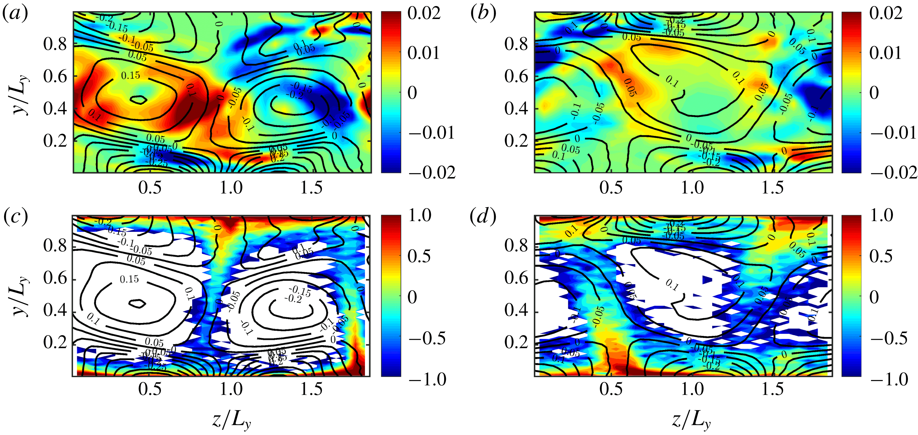
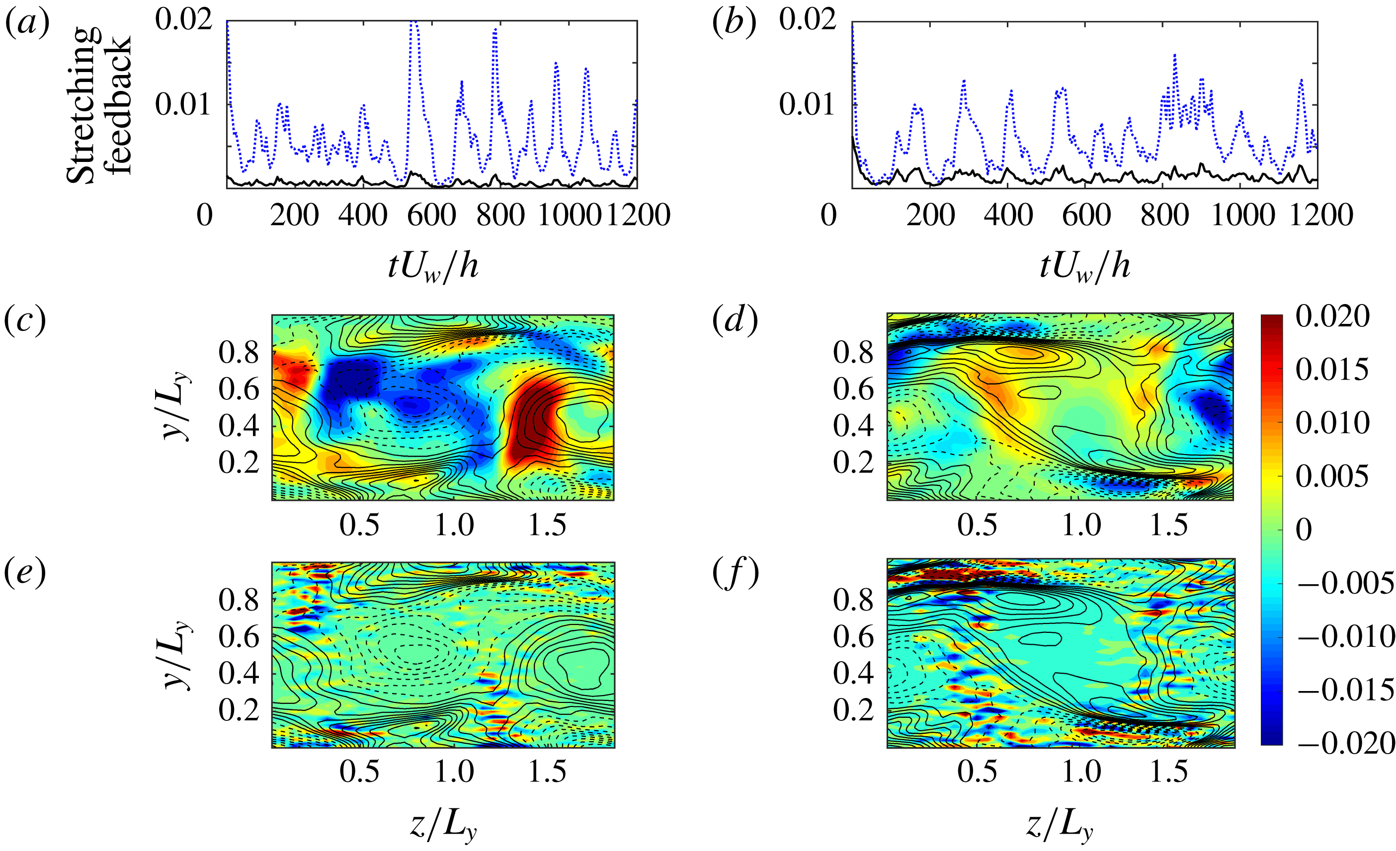
(a,b) Contour of temporal average of streamwise vortex stretching term in one single cross-section (
 $y,z$
plane) within
 $50$
time units and isolines of temporal and streamwise average of streamwise vorticity within
 $50$
time units. (c,d) Contour (logarithmic scale) of temporal and streamwise average of normalized concentration by the bulk value and isolines of temporal and streamwise average of streamwise vorticity within
 $50$
time units. (a,c) Case 500–500–4; (b,d): case 500–900–4.

To visualize this stabilization process that occurs in the annulus of region
 $0.015<|\unicode[STIX]{x1D714}_{x}|<0.1$
, figure 5(a,b) shows the contour of streamwise vorticity stretching
 $\unicode[STIX]{x1D714}_{x}\unicode[STIX]{x2202}u/\unicode[STIX]{x2202}x$
. This is a streamwise-dependent quantity, so we time-average (50 time units) at a single cross-section at
 $x=L_{x}/2$
. Figure 5(c,d) shows the contour of the normalized particle concentration with respect to the bulk concentration at the same location and averaged over the same time. The isolines in all panels are the streamwise-averaged streamwise vorticity (
 $\overline{\unicode[STIX]{x1D714}_{x}}(y,z)$
). Figure 5(a,c) and figure 5(b,d) show cases 500–500–4 and 500–900–4, respectively. It is clear that strong vorticity stretching happens in the range of
 $0.015<|\unicode[STIX]{x1D714}_{x}|<0.1$
, which is a key component of the self-sustaining regeneration cycle. The intensity of this stretching is reduced in case 500–900–4 (contour in figure 5
b) compared to that of case 500–500–4 (contour in figure 5
a). Simultaneously, we find that there are more particles present in the range of
 $0.015<|\unicode[STIX]{x1D714}_{x}|<0.1$
in case 500–900–4 (figure 5
d) than in case 500–500–4 (figure 5
c).
As a result, we associate the turbulence attenuation with the streamwise coupling of high-inertia particles (e.g.
 $St_{turb}=0.625$
), and their presence in the range of
 $0.015<|\unicode[STIX]{x1D714}_{x}|<0.1$
is of key significance since this is the region which has the strongest streamwise vortex stretching effect. Below, we argue that the streamwise vortex stretching and the LSVs are the key sub-steps in the regeneration cycle, and coupled to each other. The preferential presence of particles in this streamwise vortex stretching region is an important phenomenon which alters the regeneration cycle and thus the transition from turbulent to laminar flow, and has been observed at higher Reynolds numbers (Lee & Lee Reference Lee and Lee2015).
3.3 Particle distribution and velocity profile
For inertial pointwise particles, their spatial distribution is determined through the drag force exerted from large-scale turbulent structures to the particles. Due to inertia, heavy particles tend to be expelled from the vortex centre to the low-vorticity but high-strain-rate regions (Druzhinin & Elghobashi Reference Druzhinin and Elghobashi1998). As argued above, this process plays a key role in turbulence modulation since particles tend to accumulate in regions associated with streamwise vortex stretching. In a similar study focused on neutrally buoyant finite-sized particles, Wang et al. (Reference Wang, Abbas and Climent2018) found that particles accumulating in the streaks tend to enhance the turbulence whereas particles accumulating in the large-scale rolls hardly modify turbulence levels.
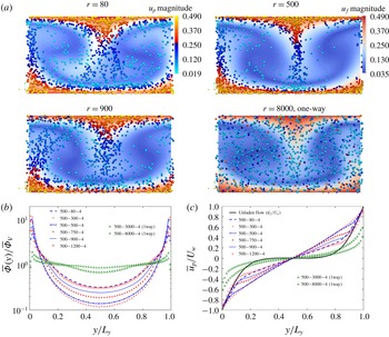
(a) Contours of the magnitude of the streamwise flow velocity (colourbar in upper left panel) and instantaneous particle positions projected onto the
 $(y,z)$
cross-section when the LSS is strongest before breakdown, coloured according to magnitude of particle streamwise velocity (colourbar in upper right panel). The particle size shown in the panels is magnified four times for better visualization. Top-left: case 500–80–4; top-right: case 500–500–4; bottom-left: case 500–900–4; bottom-right: case 500–8000–4 (one-way coupling). (b) Mean volume concentration normalized by the bulk concentration. (c) Mean streamwise velocity scaled by
 $U_{w}$
.

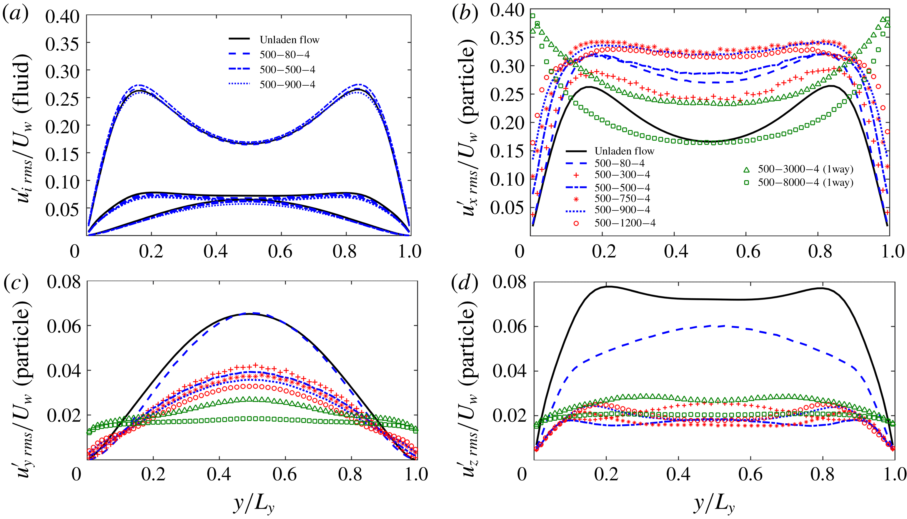
RMS velocity fluctuations in cases with density ratios. (a) Fluid phase in three directions. (b–d) Particulate phase in three directions: (b) streamwise direction fluctuation; (c) wall-normal direction fluctuation; (d) spanwise direction fluctuation. In (b–d), fluid phase in single phase is plotted as a reference.

Figure 6(a) shows an instantaneous particle distribution over a
 $(y,z)$
cross-sectional plane with different density ratios (
 $r=80{-}8000$
) at the same Reynolds number (
 $Re_{b}=500$
) and volumetric concentration (
 $\overline{\unicode[STIX]{x1D6F7}_{v}}=4\times 10^{-4}$
) at a point in time corresponding to the strongest LSSs during the regeneration cycle. From left to right, top to bottom, it is clear that particles with low to moderate inertia tend to accumulate in the LSSs whereas particles with a higher inertia distribute more homogeneously and spread throughout the Couette gap, a behaviour seen in other particle-laden, wall-bounded turbulent flows. Along the same lines, particles with density ratio from
 $r=300$
to
 $500$
are mostly trapped inside the LSSs, even during the streak breakdown process (not shown). Either lower (e.g.
 $r=80$
) or higher (e.g.
 $r=900$
) than this density ratio, the particles can stray from the LSS regions, consistent with known behaviour of inertial particles (Maxey Reference Maxey1987; Druzhinin & Elghobashi Reference Druzhinin and Elghobashi1998). In a Taylor–Green vortex (TGV) set-up, Massot (Reference Massot2007) proposed a threshold of the ratio between particle response time and the TGV turnover time scale. Below the threshold, particles will stay inside this cell whereas particles tend to move to the other cells above the value. We numerically obtained the single-particle trajectory in TGV flow with the same particle time scale corresponding to particles in the present simulated turbulent LSVs. The particle behaviour in TGV flow is analogous to particle distribution in turbulent PCF with the same particle time scale (data are not shown here). Case 500–80–4 has a low
 $St_{turb}\approx 0.056$
causing the particles to behave more as tracers and stay in one LSV, whereas case 500–8000–4(1way) with a high
 $St_{turb}\approx 5.56$
leads to particles which cannot follow the streamlines and cross the LSVs after being ejected by ejection events. Particles with intermediate Stokes numbers, as in case 500–500–4 with
 $St_{turb}\approx 0.35$
, are expelled from the LSVs and become trapped inside the LSSs.
This non-monotonic change in particle distribution can be seen in figure 6(b), where the normalized particle volume concentration is shown. With increasing density ratio from 500–80–4 to 500–300–4, the concentration decreases in the centre whereas it increases in the near-wall region. We observe an opposite tendency when further increasing the density ratio from 500–300–4 to 500–1200–4. At higher density ratios with two-way coupling, transition to laminar flow occurs in the present simulations. At higher flow Reynolds number (
 $Re_{b}=2025$
), the increase of particle concentrations in the centre with increasing particle response time (
 $\unicode[STIX]{x03C4}_{p}^{+}\approx 90$
corresponding to
 $St_{turb}\approx 1.06$
) is also observed by Richter & Sullivan (Reference Richter and Sullivan2013). For the sake of highlighting the long particle response time effect on the particle distribution, we also show cases 500–3000–4 and 500–8000–4 with one-way coupling, where we can find a nearly homogeneous concentration profile because particles cannot follow the streamlines.
Despite the slip velocity between the particulate phase and fluid phase, the shape of the mean particle velocity profile is mainly determined by the carrier phase. In particular, the mean particle streamwise velocity will reflect the local mean fluid velocity profile of the structure it is contained within (e.g. LSSs or LSVs). Hamilton et al. (Reference Hamilton, Kim and Waleffe1995) have shown that for the miniunit configuration, the characteristic ‘S’ shape of the mean velocity profile in PCF is governed primarily by the LSVs in single-phase flow. Figure 6(c) compares the mean fluid velocity (solid black line) to the mean particle velocities
 $\overline{u_{p}}/U_{w}$
of particles with varying density. There is a clear distinction between the nearly linear (respectively ‘S’) shape of the mean particle velocity curve for 500–300–4 (respectively 500–3000–4(1way)) if the particles are trapped in the LSSs (respectively across the whole domain). Again, this effect is non-monotonic with particle inertia. For cases 500–3000–4(1way) and 500–8000–4(1way), the qualitative shape of the mean particle velocity is similar to that of mean fluid velocity in single-phase flow; this discrepancy is due to the difference between the particle response time scale and the turnover time of the LSV.
3.4 Turbulence intensity
The RMS velocity fluctuations for the various cases are plotted in figure 7. Figure 7(a) shows the RMS velocities in all three directions for the fluid phase, where it is apparent that
 $u_{f\,rms}^{\prime }$
is nearly unchanged whereas in the core region
 $v_{f\,rms}^{\prime }$
and
 $w_{f\,rms}^{\prime }$
decrease slightly with increased particle inertia. The particulate RMS velocity fluctuations are shown in figure 7(b–d); the single-phase velocity fluctuations are also plotted as a reference (solid black lines). As noted by Yu, Vinkovic & Buffat (Reference Yu, Vinkovic and Buffat2016), particles moving away from the wall are associated mainly with ejections while particles moving towards the wall are associated with sweeps. As seen above, inertial particles with low to moderate Stokes numbers tend to remain in the high-strain-rate region (see figure 6) – regions associated with high
 $u_{f\,rms}^{\prime }$
. This results in high values of
 $u_{p\,rms}^{\prime }$
across the whole Couette flow gap which can be seen in figure 7(b). Thus the increase of particulate streamwise turbulent kinetic energy compared with single-phase flow is due to the accumulation of particles in the LSS which contains high streamwise turbulent kinetic energy.
The effect is opposite for
 $v_{p\,rms}^{\prime }$
and
 $w_{p\,rms}^{\prime }$
. The fluid velocity fluctuations
 $v_{f\,rms}^{\prime }$
and
 $w_{f\,rms}^{\prime }$
are high in the outer regions of the LSVs (not shown here). Therefore when the inertial particles collect in high-strain-rate regions (intermediate Stokes numbers), their spanwise and wall-normal velocity fluctuations are much smaller than the fluid average. At low Stokes numbers, long residence times in the LSVs allow particles to gain wall-normal and spanwise kinetic energy (figure 7
c,d). At high Stokes number, particles tend to again distribute homogeneously throughout the whole domain. Particles move across LSVs, but their inability to quickly adjust their velocity results in suppressed values of
 $v_{p\,rms}^{\prime }$
and
 $w_{p\,rms}^{\prime }$
.
As a final note, we have compared the particle distribution, mean velocity and RMS velocity fluctuations (not shown here) between case 500–80–4 and a simulation with finite-size particles from Wang et al. (Reference Wang, Abbas and Climent2017); both have the same particle response time. We find that even for the same Stokes number, finite-size particles collect more in the central region and that their mean velocity and fluctuations are similar to the fluid phase. This difference is due directly to finite-size effects which should be considered for physical systems where particle diameters are larger than the dissipation scales of the flow.
4 Modal analysis of the regeneration cycle modulation
Turbulence regeneration mechanisms in wall turbulence involve three-dimensional, multiscale structures, and the relevant nonlinear dynamics involved is neglected when performing linear stability analyses on laminar-to-turbulent transition and streak stability. Therefore to leverage the present nonlinear simulations, modal analysis is used to determine the natural mode shapes and frequencies in this miniunit PCF system – this strategy significantly simplifies the range of temporal and length scales in the turbulent flow, thereby highlighting the essential features (e.g. LSSs and LSVs) in the regeneration cycle. To start, it is helpful to provide a list of relevant quantities which are useful in defining the various stages/structures of the regeneration cycle, which will be further analysed in this section.
(i) The turbulent kinetic energy contained in the streaks and its corresponding Fourier modes yield information about the contributions from various scales in the flow. We define
 ${\mathcal{M}}(k_{x}=m\unicode[STIX]{x1D6FC},k_{z}=n\unicode[STIX]{x1D6FD})$
as the vertically integrated modal RMS velocity modes in the two periodic directions (
 $x$
and
 $z$
), following Hamilton et al. (Reference Hamilton, Kim and Waleffe1995):
 $$\begin{eqnarray}{\mathcal{M}}(m\unicode[STIX]{x1D6FC},n\unicode[STIX]{x1D6FD})\equiv \left\{\int _{0}^{L_{y}}[\widehat{u^{\prime }}^{2}(m\unicode[STIX]{x1D6FC},y,n\unicode[STIX]{x1D6FD})+\widehat{v^{\prime }}^{2}(m\unicode[STIX]{x1D6FC},y,n\unicode[STIX]{x1D6FD})+\widehat{w^{\prime }}^{2}(m\unicode[STIX]{x1D6FC},y,n\unicode[STIX]{x1D6FD})]\,\text{d}y\right\}^{1/2},\end{eqnarray}$$
where
 $(\unicode[STIX]{x1D6FC},\unicode[STIX]{x1D6FD})$
are the fundamental wavenumbers in the streamwise and spanwise directions (defined as
 $(2\unicode[STIX]{x03C0}/L_{x},2\unicode[STIX]{x03C0}/L_{z})$
), and
 $m$
and
 $n$
are integers. In principle, each mode
 $(m\unicode[STIX]{x1D6FC},n\unicode[STIX]{x1D6FD})$
provides information about specific structures in the flow. For instance in the miniunit domain (note that this may not necessarily be true in full domains):
 ${\mathcal{M}}(0,\unicode[STIX]{x1D6FD})$
represents the LSSs since it is the zeroth mode in the streamwise direction, and any mode
 $(0,n\unicode[STIX]{x1D6FD})$
with
 $n\neq 0$
is an
 $x$
-independent structure;
 ${\mathcal{M}}(\unicode[STIX]{x1D6FC},0)$
represents meandering streaks where the other
 ${\mathcal{M}}(m\unicode[STIX]{x1D6FC},n\unicode[STIX]{x1D6FD})$
with
 $n\neq 0$
modes are very weak.
(ii) Circulation represents the intensity of the LSVs in the miniunit. Hamilton & Abernathy (Reference Hamilton and Abernathy1994) and Hamilton et al. (Reference Hamilton, Kim and Waleffe1995) stipulated that over one cycle, vortices must have a maximum circulation above a given threshold in order to produce an LSS through the lift-up process. Thus this integrated quantity provides a good measure of whether or not this essential process can occur. The circulation of the streamwise vortices of mode zero in the streamwise direction (
 $x$
-independent) and mode
 $n\neq 0$
in the
 $z$
direction (
 $z$
-dependent) is given by
 $$\begin{eqnarray}{\mathcal{C}}(0,n\unicode[STIX]{x1D6FD})\equiv \int _{0}^{L_{y}}\hat{\unicode[STIX]{x1D714}}_{x}(0,y,n\unicode[STIX]{x1D6FD})\,\text{d}\boldsymbol{S}(\boldsymbol{n}),\end{eqnarray}$$
where
 $\boldsymbol{S}(\boldsymbol{n})\equiv \text{d}y\cdot L_{z}/n$
is the transverse surface with
 $y$
varying from
 $0$
to
 $L_{y}$
and
 $z$
varying from
 $0$
to
 $2\unicode[STIX]{x03C0}/(n\unicode[STIX]{x1D6FD})$
for
 $n\neq 0$
. Based on our calculations, the maximum circulation in the miniunit domain always corresponds to
 $n=1$
, and therefore we define circulation as
 ${\mathcal{C}}(0,\unicode[STIX]{x1D6FD})$
and use this measure to stand for the intensity of LSVs.
(iii) Lift-up: in the buffer layer, elongated streaks form on both sides of an LSV (see figure 6 a). The so-called lift-up effect has been identified as a very robust mechanism for the generation of streaky motions in both transitional and turbulent flows (Ellingsen & Palm Reference Ellingsen and Palm1975; Hamilton et al. Reference Hamilton, Kim and Waleffe1995; Brandt Reference Brandt2014). Fluid in the near-wall region is lifted away from the wall by the longitudinal vortical structures into a region of higher-speed fluid (so-called ejection), producing a low-speed streak. Simultaneously on the other side of the vortex, high-speed fluid is pushed towards the wall (so-called sweep), creating a high-speed streak. Consequently in shear flows, the main linear mechanism for transient disturbance growth is the lift-up effect that produces low- and high-speed streaks in the streamwise velocity (Ellingsen & Palm Reference Ellingsen and Palm1975). Bech et al. (Reference Bech, Tillmark, Alfredsson and Andersson1995) stated that the inner shear layer is formed via the lift-up of low-speed streaks from the viscous sub-layer. Once this occurs, the shear layers are coupled to an instantaneous velocity profile with an inflectional character, and they have been observed to become unstable and break up into chaotic motion, so-called ‘bursting’. Specifically in Fourier space, Hamilton et al. (Reference Hamilton, Kim and Waleffe1995) have shown that the term most responsible for extracting energy from the mean shear flow is given by
 $$\begin{eqnarray}{\mathcal{L}}(0,n\unicode[STIX]{x1D6FD})\equiv \int _{0}^{L_{y}}\widehat{v^{\prime }}(0,y,n\unicode[STIX]{x1D6FD})\frac{\unicode[STIX]{x2202}U(y)}{\unicode[STIX]{x2202}y}\,\text{d}y,\end{eqnarray}$$
where
 $\widehat{v^{\prime }}$
is the wall-normal fluctuation velocity in Fourier space and
 $\unicode[STIX]{x2202}U(y)/\unicode[STIX]{x2202}y$
is the gradient of the mean steamwise velocity.
(iv) Steamwise vortex stretching: during streak breakdown, nonlinear interactions reinforce the streamwise LSVs, leading to the formation of a new set of streaks, and completing the regeneration cycle. Hamilton et al. (Reference Hamilton, Kim and Waleffe1995) proposed that the strengthening of the vortices is due to interactions among the
 $\unicode[STIX]{x1D6FC}$
-modes, which grow during the streak breakdown. Schoppa & Hussain (Reference Schoppa and Hussain2002) suggested that the vortex formation is inherently three-dimensional, with direct stretching (inherent to streak
 $(x,z)$
-waviness) of near-wall
 $\unicode[STIX]{x1D714}_{x}$
sheets leading to streamwise vortex collapse. They provided insights into the dynamics of near-wall vortex formation through the inviscid equation for streamwise vorticity:
 $$\begin{eqnarray}\frac{\unicode[STIX]{x2202}\unicode[STIX]{x1D714}_{x}}{\unicode[STIX]{x2202}t}=\underbrace{-u\frac{\unicode[STIX]{x2202}\unicode[STIX]{x1D714}_{x}}{\unicode[STIX]{x2202}x}-v\frac{\unicode[STIX]{x2202}\unicode[STIX]{x1D714}_{x}}{\unicode[STIX]{x2202}y}-w\frac{\unicode[STIX]{x2202}\unicode[STIX]{x1D714}_{x}}{\unicode[STIX]{x2202}z}}_{\text{advection}}+\underbrace{\unicode[STIX]{x1D714}_{x}\frac{\unicode[STIX]{x2202}u}{\unicode[STIX]{x2202}x}}_{\text{stretching}}+\underbrace{\frac{\unicode[STIX]{x2202}v}{\unicode[STIX]{x2202}x}\frac{\unicode[STIX]{x2202}u}{\unicode[STIX]{x2202}z}-\frac{\unicode[STIX]{x2202}w}{\unicode[STIX]{x2202}x}\frac{\unicode[STIX]{x2202}u}{\unicode[STIX]{x2202}y}}_{\text{tilting}}+\underbrace{\frac{\unicode[STIX]{x2202}F_{z}}{\unicode[STIX]{x2202}y}-\frac{\unicode[STIX]{x2202}F_{y}}{\unicode[STIX]{x2202}z}}_{\text{particle feedback}}.\end{eqnarray}$$
In fully developed turbulent single-phase flow, the greatest contribution, in magnitude, to the temporal evolution of the vorticity
 $\unicode[STIX]{x2202}\unicode[STIX]{x1D714}_{x}/\unicode[STIX]{x2202}t$
is related to the tilting term (Sendstad & Moin Reference Sendstad and Moin1992). However, Schoppa & Hussain (Reference Schoppa and Hussain2002) have shown that this term mainly contributes to the thin tail of the near-wall
 $\unicode[STIX]{x1D714}_{x}$
layer, and is not responsible for
 $x$
-independent streamwise vortex formation (
 $(0,\unicode[STIX]{x1D6FD})$
mode in the miniunit). In particle suspension flow, an additional term named particle feedback is added in the streamwise vorticity equation representing the contribution from the inhomogeneous distribution of the feedback force from the particles to the fluid. In appendix A, we do the comparison between the contributions to LSVs with
 $(0,\unicode[STIX]{x1D6FD})$
from the stretching term and the particle feedback term within
 $20<y^{+}<60$
where the regeneration cycle happens. The contribution from the particle feedback term to the LSV formation is much less than the contribution from the stretching term (about
 $10\,\%$
in case 500–80–4 and
 $17\,\%$
in case 500–900–4). Instead, vortex formation is dominated by stretching of streamwise vorticity. The local
 $\unicode[STIX]{x1D714}_{x}$
stretching is sustained in time and is mainly responsible for the vortex collapse, whose location coincides with the
 $+\unicode[STIX]{x1D714}_{x}\unicode[STIX]{x2202}u/\unicode[STIX]{x2202}x$
peak. The meandering of streaks provides the generation of
 $\unicode[STIX]{x2202}u/\unicode[STIX]{x2202}x$
, and then direct stretching of positive and negative
 $\unicode[STIX]{x1D714}_{x}$
occurs in regions where
 $\unicode[STIX]{x2202}u/\unicode[STIX]{x2202}x$
is generated across the wavy streak flanks during the streak breakdown process. The stretching term is active only during the peaks of the cycle when local three-dimensionality is induced after streak breakdown (see Jiménez & Moin Reference Jiménez and Moin1991). In Fourier space, the stretching term can be written as
 $$\begin{eqnarray}{\mathcal{S}}(m\unicode[STIX]{x1D6FC},n\unicode[STIX]{x1D6FD})\equiv \int _{0}^{L_{y}}\widehat{\unicode[STIX]{x1D714}_{x}}(p\unicode[STIX]{x1D6FC},y,q\unicode[STIX]{x1D6FD})\frac{\unicode[STIX]{x2202}\widehat{u}(r\unicode[STIX]{x1D6FC},y,s\unicode[STIX]{x1D6FD})}{\unicode[STIX]{x2202}x}\,\text{d}y,\end{eqnarray}$$
where the total time rate of change of streamwise vorticity in the
 $(m\unicode[STIX]{x1D6FC},y,n\unicode[STIX]{x1D6FD})$
mode is the summation of terms over all values of
 $p,q,r,s$
such that
 $p+r=m$
and
 $q+s=n$
. The contribution to the LSV with
 $(0,\unicode[STIX]{x1D6FD})$
comes from wavenumber combinations which satisfy
 $p+r=0$
and
 $q+s=1$
. For the streamwise direction, Hamilton et al. (Reference Hamilton, Kim and Waleffe1995) demonstrated that
 $p=\pm 1$
and
 $r=\mp 1$
are the dominant terms producing additional streamwise vorticity in the right places where the higher
 $x$
-wavenumber modes are negligible. It is difficult, however, to specify a single pair of modes combining both
 $x$
-wavenumber and
 $z$
-wavenumber which are dominant.
Therefore, we consider all pairs
 $p=\pm 1$
and
 $r=\mp 1$
satisfying the condition
 $m=p+r=0$
in the streamwise direction and
 $q=-2$
to
 $3$
and
 $s=3$
to
 $-2$
satisfying the condition
 $n=q+s=1$
in the spanwise direction (a total
 $12$
pairs of
 $x$
and
 $z$
wavenumbers). A discrete Fourier transform can be expressed as a complex number containing the modulus and argument, and in appendix B we show the modulus of each of the
 $12$
pairs of wavenumbers and their phase differences with the meandering streak. Since the summation of these
 $12$
pairs as shown in figure 13 reflects around
 $91\,\%$
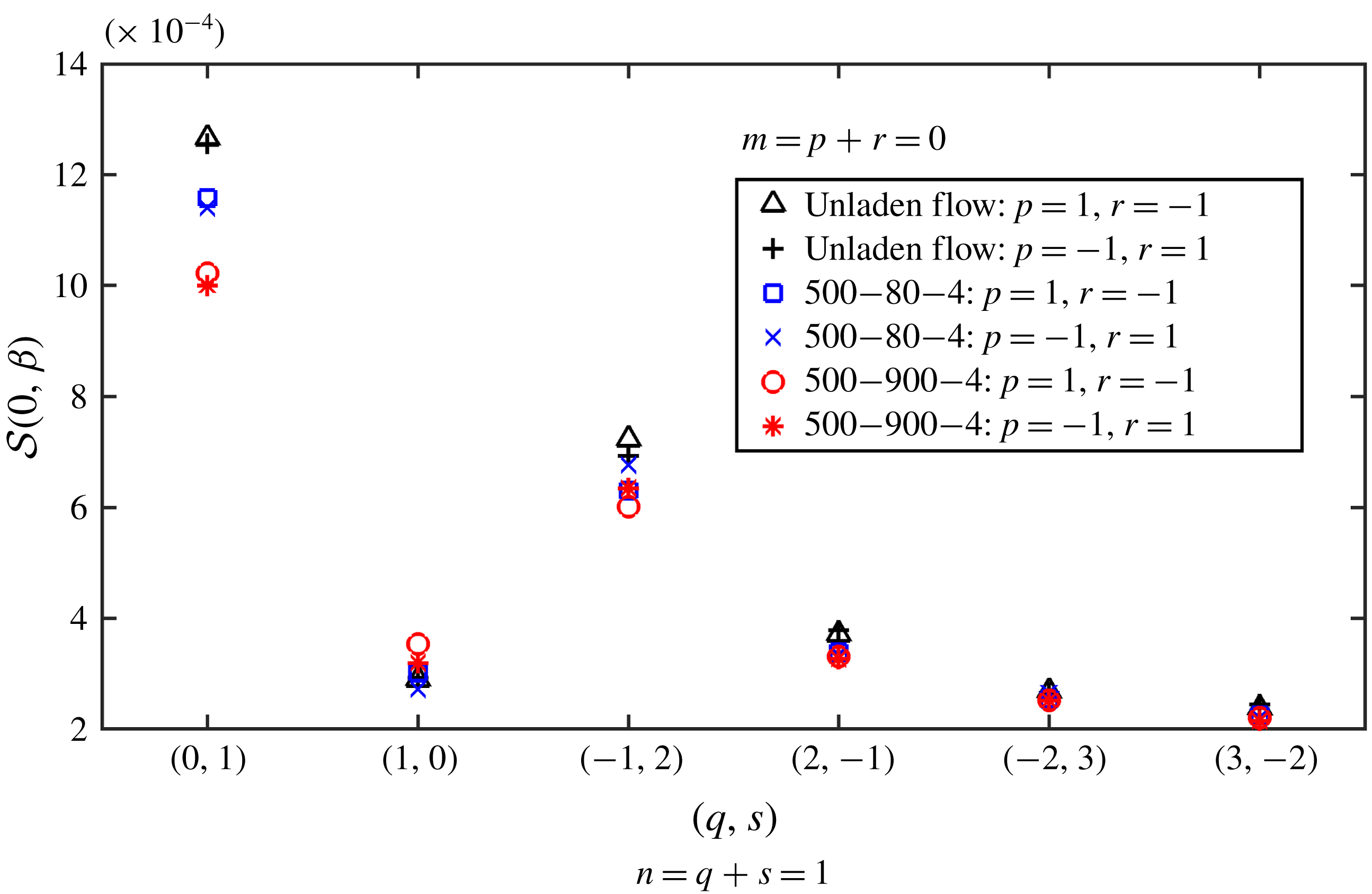
of the summation of all modes, we use this summation as a measure of the streamwise vortex stretching effect.
4.1 Intensity of the characteristic terms of regeneration cycle
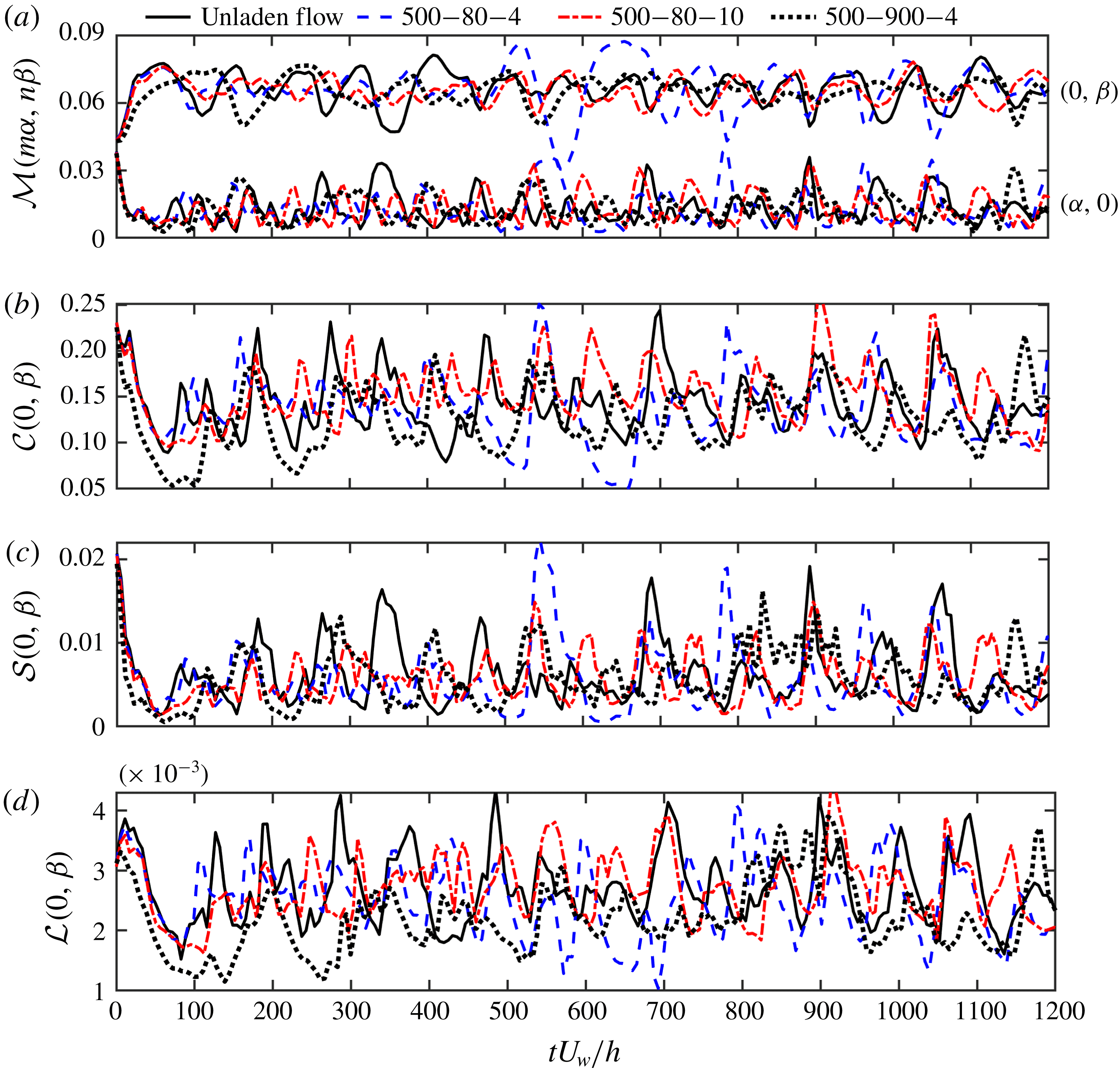
Modal decomposition of the various sub-steps composing the regeneration cycle as shown in figure 1 and outlined in § 4. Four cases are shown: 500–0–0 (unladen), 500–80 (500–80–4 and 500–80–10 with
 $St_{turb}=0.056$
, turbulence enhancement) and 500–900–4 (
 $St_{turb}=0.625$
, turbulence attenuation). (a)
 ${\mathcal{M}}(n\unicode[STIX]{x1D6FC},m\unicode[STIX]{x1D6FD})$
as in (4.1) representing turbulent kinetic energy contained in the streaks; (b)
 ${\mathcal{C}}(0,\unicode[STIX]{x1D6FD})$
as in (4.2) representing for the intensity of the LSV; (c)
 ${\mathcal{S}}(0,\unicode[STIX]{x1D6FD})$
as in (4.5) representing the vorticity stretching effect to LSV; (d)
 ${\mathcal{L}}(0,\unicode[STIX]{x1D6FD})$
representing the lift-up effect induced by LSV to enhance LSS as in (4.3). The initial
 $1200$
time units (
 $h/U_{w}$
) are shown.

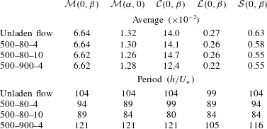
The average and period of five characteristic terms of the regeneration cycle. The error of the period due to the resolution of the signals is in the range of
 $\pm 2.5$
time units.
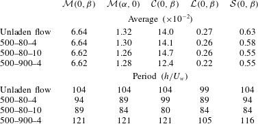
Figure 8 shows the temporal evolution of the quantities defined in the previous section: the wall-normal integrated amplitude of LSSs (
 ${\mathcal{M}}(0,\unicode[STIX]{x1D6FD})$
; figure 8
a), the strength of the meandering streak (represented by mode
 ${\mathcal{M}}(\unicode[STIX]{x1D6FC},0)$
; figure 8
a), LSV strength (represented by
 ${\mathcal{C}}(0,\unicode[STIX]{x1D6FD})$
; figure 8
b), the vortex stretching term (represented by
 ${\mathcal{S}}(0,\unicode[STIX]{x1D6FD})$
which is the summation of all 12 pairs of
 $p=\pm 1$
and
 $r=\mp 1$
in combination with
 $q=-2$
to
 $3$
and
 $s=3$
to
 $-2$
; figure 8
c) and the lift-up term (represented by
 ${\mathcal{L}}(0,\unicode[STIX]{x1D6FD})$
mode; figure 8
d). Clearly, all of the signals are fluctuating in time with a similar period corresponding to the three regeneration steps as shown in figure 1. In single-phase flow, Hamilton et al. (Reference Hamilton, Kim and Waleffe1995) estimated this period is slightly less than
 $100$
time units (
 $h/U_{w}$
) at
 $Re_{b}=500$
. In flow influenced by low-inertia finite-size particles, Wang et al. (Reference Wang, Abbas and Climent2017) also observed a similar period.
Figure 8 shows that the amplitudes of
 ${\mathcal{M}}(0,\unicode[STIX]{x1D6FD})$
and
 ${\mathcal{M}}(\unicode[STIX]{x1D6FC},0)$
are diminished by the inertial particles of case 500–900–4 (dotted black line), which is consistent with the behaviour observed by Wang et al. (Reference Wang, Abbas and Climent2017) for finite-size particles. However for low particle inertia, the amplitude of
 ${\mathcal{M}}(\unicode[STIX]{x1D6FC},0)$
is nearly unchanged due to low mass fraction (case 500–80–4) whereas it is suppressed with the presence of more particles of the same Stokes number (case 500–80–10). The presence of a large number of inertial particles (either when they enhance or attenuate the turbulence) tends to stabilize the amplitude of LSSs (
 ${\mathcal{M}}(0,\unicode[STIX]{x1D6FD})$
) but not significantly affect the time-averaged intensity of the streaks.
The time-averaged intensities of
 ${\mathcal{C}}(0,\unicode[STIX]{x1D6FD})$
,
 ${\mathcal{S}}(0,\unicode[STIX]{x1D6FD})$
and
 ${\mathcal{L}}(0,\unicode[STIX]{x1D6FD})$
are provided in table 2, where we see that these characteristic terms are all suppressed when turbulence attenuation occurs due to particles (case 500–900–4). However, for cases with turbulence enhancement (cases 500–80–10 and 500–80–4), the primary difference is the amplified intensity of the circulation (
 ${\mathcal{C}}(0,\unicode[STIX]{x1D6FD})$
, also seen in figure 8
b), and this amplification increases with particle concentration. The strengthened LSVs are critical for sustaining the turbulence and thus are consistent with the observed lower transitional Reynolds number (
 $Re_{c}\sim 290$
in case 500–80–4 versus
 $Re_{c}\sim 320$
for single-phase flow as shown in figure 3
a). As found by Hamilton & Abernathy (Reference Hamilton and Abernathy1994), there is a minimum threshold of circulation below which the turbulence collapses and the flow becomes laminar. At lower Reynolds numbers and/or higher particle concentrations, we indeed see that this is the case (not shown here), and it appears that the primary effect of the particles is to modify the LSV strength during both stabilization and destabilization.
4.2 Periodic behaviour and phase difference of the regeneration cycle
To better understand the effects of particles on the timing of the regeneration cycle, we calculate a temporal autocorrelation of the five signals in figure 8:
 $$\begin{eqnarray}R_{ss}(\unicode[STIX]{x0394}t)=\frac{\overline{s^{\prime }(t)s^{\prime }(t+\unicode[STIX]{x0394}t)}}{s_{rms}^{\prime ^{2}}},\end{eqnarray}$$
where
 $s^{\prime }$
is the fluctuation of a signal with respect to the time-averaged value.
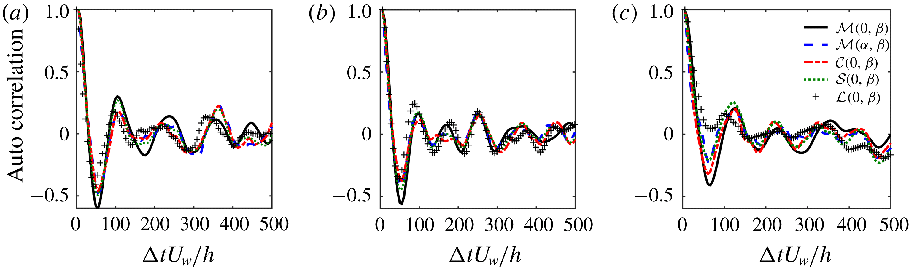
Temporal autocorrelation functions of the five signals shown in figure 8. (a) Single-phase flow, case 500–0–0. Suspension flow: (b) case 500–80–4; (c) case 500–900–4.

The temporal autocorrelation is calculated over
 $3600$
time units to ensure converged statistics. Figure 9(a) plots the five temporal autocorrelations in single-phase flow, case 500–80–4 is shown in figure 9(b) and case 500–900–4 is shown in figure 9(c). The time difference between the first two maxima of the correlation coefficient is taken as the period of the cycle and these are summarized in table 2. We can see that the period changes due to the presence of the particles, and that in cases of turbulence enhancement, the period is shortened (similar phenomenon is observed by Pan & Banerjee (Reference Pan and Banerjee1996), where particles enhance the turbulence with an increasing frequency of the sweep activity), while for turbulence suppression, the period is lengthened. Along these lines, in single-phase flow, Hamilton et al. (Reference Hamilton, Kim and Waleffe1995) observed that the period of the regeneration cycle is shortened at lower Reynolds numbers, e.g. 18 cycles in 1500 time units at
 $Re_{b}=400$
versus 16 cycles in 1500 time units at
 $Re_{b}=500$
. Therefore comparing to single-phase flow, the period of the regeneration cycle increases in case 500–900–4 (turbulence is attenuated, behaving as a lower Reynolds in single-phase flow) whereas the period of the regeneration cycle decreases in cases 500–80–4 and 500–80–10 (turbulence is enhanced, behaving as a higher Reynolds in single-phase flow).
The regeneration cycle consists of three sequential sub-processes sketched in figure 1: streak formation, streak breakdown and streamwise vortex regeneration. The key mechanisms are: the LSSs are generated by a linear lift-up process by the LSVs, the LSSs break down to meandering streaks by complex nonlinear interactions and wavy streaks (
 $x$
-dependent, contributing to
 $\unicode[STIX]{x2202}u/\unicode[STIX]{x2202}x$
) interact with streamwise vorticity (
 $\unicode[STIX]{x1D714}_{x}$
) to strengthen the LSVs, which is another nonlinear process. This cycle is recognized as a robust, spatial–temporal evolution and time-stable self-sustaining process. We noted above that the period of this cycle (e.g. signal
 ${\mathcal{M}}(0,\unicode[STIX]{x1D6FD})$
) is around
 $104$
time units in single-phase flow,
 $94$
time units in case 500–80–4 and
 $121$
time units in case 500–900–4. It is instructive to further analyse the phase difference during the regeneration cycle, especially in order to quantify the inertial particle effect during turbulence modulation. As can be seen in figure 8, the LSSs (
 ${\mathcal{M}}(0,\unicode[STIX]{x1D6FD})$
) and the meandering streaks (
 ${\mathcal{M}}(\unicode[STIX]{x1D6FC},0)$
) nearly have opposite phase. Two subsequent sub-steps, the vortex stretching (
 ${\mathcal{S}}(0,\unicode[STIX]{x1D6FD})$
) and the lift-up (
 ${\mathcal{L}}(0,\unicode[STIX]{x1D6FD})$
) induced by LSVs, are closely synchronous with the temporal evolution of circulation (
 ${\mathcal{C}}(0,\unicode[STIX]{x1D6FD})$
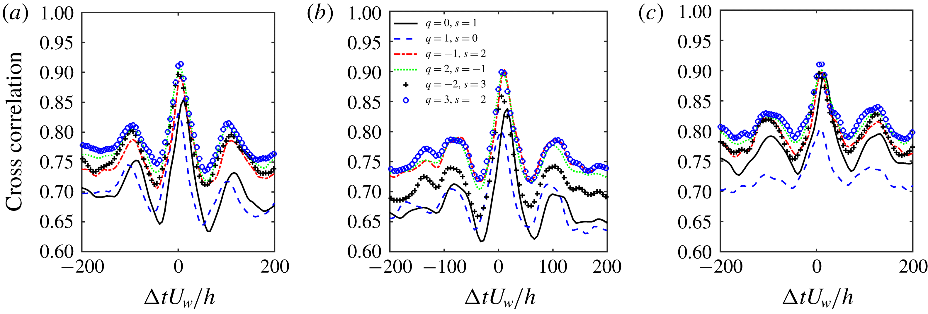
). Vortex stretching, lift-up and circulation all seem to remain in phase with the meandering streaks. To verify this, we perform a temporal cross-correlation study of the five signals based on (4.7):
 $$\begin{eqnarray}R_{s_{1}s_{2}}(\unicode[STIX]{x0394}t)=\frac{\overline{s_{1}^{\prime }(t+\unicode[STIX]{x0394}t)s_{2}^{\prime }(t)}}{s_{1\,rms}^{\prime }s_{2\,rms}^{\prime }},\end{eqnarray}$$
where
 $s_{1}^{\prime }$
and
 $s_{2}^{\prime }$
are the fluctuations of signals
 $s_{1}$
and
 $s_{2}$
with respect to the time-averaged value. For instance,
 $R({\mathcal{M}}(0,\unicode[STIX]{x1D6FD}),{\mathcal{M}}(\unicode[STIX]{x1D6FC},0))$
represents temporal cross-correlation between
 ${\mathcal{M}}(0,\unicode[STIX]{x1D6FD})$
(LSS) and
 ${\mathcal{M}}(\unicode[STIX]{x1D6FC},0)$
(meandering streaks), thereby providing information on temporal lag between the two processes. If
 $R({\mathcal{M}}(0,\unicode[STIX]{x1D6FD}),{\mathcal{M}}(\unicode[STIX]{x1D6FC},0))$
is positive, it reflects that
 ${\mathcal{M}}(0,\unicode[STIX]{x1D6FD})$
occurs prior in time to
 ${\mathcal{M}}(\unicode[STIX]{x1D6FC},0)$
during one regeneration cycle – the physical explanation for this specific case is that the LSS is formed, and subsequently breaks down into meandering streaks.
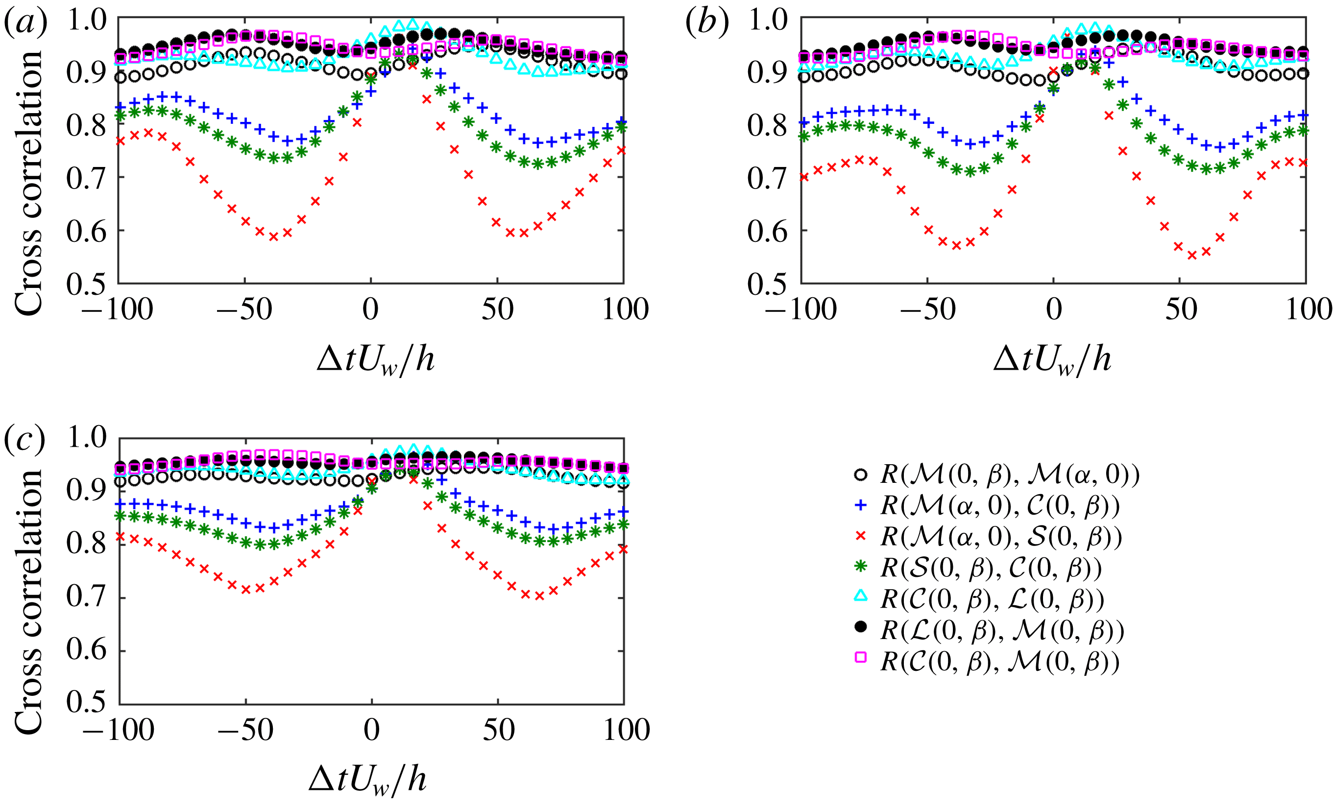
Temporal cross-correlation functions of the five signals shown in figure 8. (a) Single-phase flow, case 500–0–0. (b) Suspension flow, case 500–80–4. (c) Suspension flow, case 500–900–4. More than
 $3000$
time units of phase shifts are calculated but only the range of
 $-100$
to
 $100$
time units is shown.

Time difference (time units) between connected sub-steps of the regeneration cycle. The error due to the resolution of the signals is in the range of
 $\pm 2.5$
time units.

Figure 10 illustrates the phase difference between
 ${\mathcal{M}}(0,\unicode[STIX]{x1D6FD})$
,
 ${\mathcal{M}}(\unicode[STIX]{x1D6FC},0)$
,
 ${\mathcal{C}}(0,\unicode[STIX]{x1D6FD})$
,
 ${\mathcal{S}}(0,\unicode[STIX]{x1D6FD})$
and
 ${\mathcal{L}}(0,\unicode[STIX]{x1D6FD})$
averaged over
 $3600$
time units. Starting from the LSS (
 ${\mathcal{M}}(0,\unicode[STIX]{x1D6FD})$
) stage, we have chosen seven correlation coefficients between every pair of connected sub-steps. Figure 10(a) shows these coefficients for single-phase flow, in figure 10(b) for case 500–80–4 and in figure 10(c) for case 500–900–4. We quantify the phase shifts in table 3. Although inertial particles in case 500–900–4 have been found to attenuate the turbulence activity, the inertial particles actually do not significantly alter the basic regeneration cycle or its timing. The shortened or lengthened period of the regeneration cycle is mainly due to the particle modulation of streak breakdown from
 ${\mathcal{M}}(0,\unicode[STIX]{x1D6FD})$
(LSS) to
 ${\mathcal{M}}(\unicode[STIX]{x1D6FC},0)$
(meandering streaks) and streak formation from
 ${\mathcal{C}}(0,\unicode[STIX]{x1D6FD})$
(LSV) to
 ${\mathcal{M}}(0,\unicode[STIX]{x1D6FD})$
(LSS). Here we should point out that the vortex regeneration is not necessary for every cycle; it might be absent for some cycles (Hamilton et al.
Reference Hamilton, Kim and Waleffe1995), but its minimum value has to be above a threshold to produce unstable streaks.
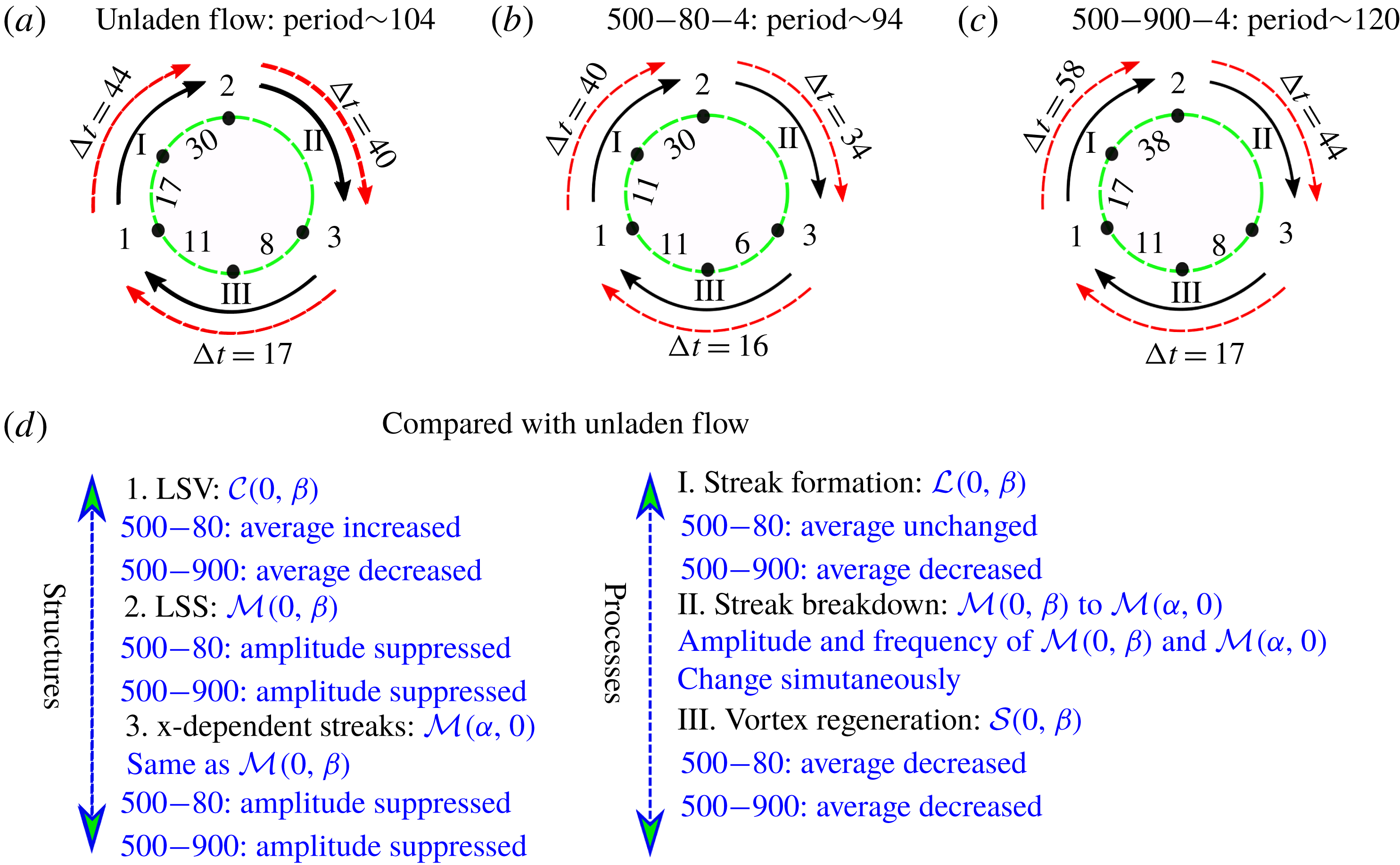
Sketch of phase difference between connected sub-steps and the period of the regeneration cycle in minimal unit: (a) case 500–0–0 in comparison with (b) case 500–80–4 and (c) case 500–900–4. (d) Qualitative comparison of the averaged value and the amplitude of the signals with single-phase flow.

Finally, we can summarize the primary effect of inertial particles on turbulence regeneration by continuing to use case 500–80 (including 500–80–4 and 500–80–10 with
 $St_{turb}=0.056$
) and case 500–900–4 (
 $St_{turb}=0.625$
) as representative examples of turbulence enhancement and turbulence attenuation, respectively. A temporal evolution of the regeneration cycle can be seen in the schematic sketch in figure 11(a–c). In this figure, we highlight the key turbulent structures and sub-steps by their corresponding metrics. The summation of the transition from
 ${\mathcal{M}}(0,\unicode[STIX]{x1D6FD})$
to
 ${\mathcal{M}}(\unicode[STIX]{x1D6FC},0)$
, from
 ${\mathcal{M}}(\unicode[STIX]{x1D6FC},0)$
to
 ${\mathcal{C}}(0,\unicode[STIX]{x1D6FD})$
and from
 ${\mathcal{C}}(0,\unicode[STIX]{x1D6FD})$
to
 ${\mathcal{M}}(0,\unicode[STIX]{x1D6FD})$
yields roughly
 $101$
time units in single-phase flow,
 $90$
time units in case 500–80–4 and
 $119$
time units in case 500–900–4 corresponding to the whole period
 $104$
time units,
 $94$
time units and
 $120$
time units, respectively. Taking into consideration the resolution of signals, it is reasonable to believe that the summed phase differences are consistent with the calculated period of the regeneration cycle.
The regeneration cycle is therefore a temporal sequence of processes which has a stable periodicity, even under the influence of inertial particles – phase differences between linked sub-steps are nearly unchanged by the presence of particles except streak formation and breakdown. Instead, during turbulence enhancement (case 500–80), as can be seen in figure 11(d), the particles simply strengthen the magnitude of the LSVs (
 ${\mathcal{C}}(0,\unicode[STIX]{x1D6FD})$
), whereas during turbulence attenuation (case 500–900–4), the particles substantially reduce the magnitude of key turbulent structures and their corresponding sub-steps. Once the magnitude of the LSVs (
 ${\mathcal{C}}(0,\unicode[STIX]{x1D6FD})$
) is below a certain threshold (as in case 380–900–4), particles act to abruptly shut off the regeneration, thereby delaying turbulent-to-laminar transition. It is worth noting that a similar upward shift of the transitional Reynolds owing to the vortex suppression is also observed during turbulence modulation laden with polymer additives – the modifications to the ‘exact coherent states’ are due to the suppression of the streamwise vortices due to the polymers exerting an opposite force to the fluid motion in the vortices and weakening the streamwise vortices (see Stone et al.
Reference Stone, Roy, Larson, Waleffe and Graham2004).
5 Concluding remarks
This work investigates the effect of inertial pointwise particles on the self-sustained process of the coherent structures in turbulent PCF. A ‘miniunit’ configuration with a low Reynolds number slightly above the onset of transition not only highlights the key turbulent structures making up the regeneration cycle, but can be simulated with much reduced computational cost. Two-way coupling of Lagrangian point particles with direct numerical simulations of Eulerian fluid flow is the methodology used in this work.
Through examining the particle inertial effect on transition, we find that lower particle inertia tends to advance the transition from laminar to turbulent flow whereas high particle inertia tends to delay the transition. These two limiting cases reflect the competition between the destabilization of the extra mixed-phase density and the stabilization due to the extra dissipation caused by the particle drag. While the nonlinear simulations capture features such as preferential accumulation, these results are in qualitative agreement with the previous linear stability analysis with assuming uniformly distributed particles. In agreement with other studies of particle-laden, wall-bounded turbulent flow, the particle response time alters where they tend to collect. The particle spatial distribution in turbulence is found to relate to the particle response time scaled by the characteristic LSV turnover time, which in turn affects the regeneration cycle. In the present domain, particles can reside either in the so-called LSS regions (high strain) or in the LSV regions (high vorticity). Low particle inertia (e.g.
 $St_{turb}=0.056$
) leads to long residence times in the same LSV, whereas high particle inertia (e.g.
 $St_{turb}=0.625$
) results in particles crossing the LSVs leading to a more homogeneous particle distribution. Between these extremes, particles with a moderate response time scale (e.g.
 $St_{turb}=0.347$
) are expelled from the LSVs and then collect in the LSSs leading to more particles accumulating in the near-wall region.
The particulate turbulent kinetic energy is highly related to particle spatial distribution and the associated slip velocity. Due to the preferential distribution of moderate-inertia particles (e.g.
 $St_{turb}=0.347$
) in the LSSs, the particulate turbulent kinetic energy is higher than that of the fluid in the streamwise direction whereas it is lower in wall-normal and spanwise directions. Particles with a large response time scale (e.g.
 $St_{turb}=0.625$
) cannot follow the streamlines, resulting in a more homogeneous distribution, which results in a more homogeneous turbulent kinetic energy of the particulate phase; however, it still exceeds the fluid phase kinetic energy in the steamwise direction.
Modal analysis is performed to examine the effect of the particles on the nonlinear regeneration cycle. For a representative set of cases at
 $Re_{b}=500$
, we quantitatively obtain its period to be roughly
 $104$
time units in single-phase flow (case 500–0–0), whereas the period is around
 $94$
time units in case 500–80–4 (turbulence enhancement happens in this case with
 $St_{turb}=0.056$
), and the period is around
 $121$
time units in case 500–900–4 (turbulence attenuation happens in this case with
 $St_{turb}=0.625$
). Furthermore, the phase differences between the linked sub-steps are obtained based on the maximum cross-correlation coefficient. The duration of each sub-step of the cycle as a fraction of the whole period of the regeneration cycle is about
 $43\,\%$
(respectively
 $44\,\%$
and
 $48\,\%$
) from LSV to LSS,
 $40\,\%$
(respectively
 $38\,\%$
and
 $38\,\%$
) from LSS to meandering streaks and
 $17\,\%$
(respectively
 $18\,\%$
and
 $14\,\%$
) from meandering streaks to LSV, in single-phase flow (respectively 500–80–4 and 500–900–4). The vortex regeneration process (from meandering streaks to LSV) is very fast whereas the lift-up process and streak breakdown process are relatively slow. The low-inertia particles (e.g.
 $St_{turb}=0.056$
) enhance the turbulence which shortens the period of the regeneration cycle whereas the high-inertia particles (e.g.
 $St_{turb}=0.625$
) attenuate the turbulence which lengthens the period of the regeneration cycle.
Even though inertial particles are found to have little effect on the phase differences between the linked sub-steps compared with the whole period, the intensity of circulation, lift-up and streamwise vorticity stretching are greatly suppressed (the reductions are about
 $15\,\%$
compared to single-phase flow in case 500–900–4) due to the presence of heavy inertial particles (e.g.
 $St_{turb}=0.625$
). The reduced intensity of circulation does not directly change the mean value of the streaks, while the amplitude of the LSSs is stabilized significantly due to the suppression of the LSVs following a suppressed lift-up effect. During turbulence attenuation by heavy inertial particles, the simulations show that it is streamwise particle–fluid coupling in an annulus region in the outer region of the LSVs coinciding with the region where streamwise vortex stretching is most active that plays the key role in suppressing the streamwise vortex stretching term and further deceasing the LSVs. However, during turbulence enhancement in cases 500–80, the circulation of LSVs is strengthened so that the minimum circulation threshold happens at a lower transition Reynolds number.
Acknowledgement
The authors acknowledge grant G00003613-ArmyW911NF-17-0366 from the US Army Research Office for financial support. Computational resources were provided by the Notre Dame Center for Research Computing. We are very grateful to Dr J. Capecelatro of the University of Michigan who provided valuable code validation resources and discussions. G.W. is grateful to Dr M. Abbas of Laboratoire de Génie Chimique (LGC) and Dr E. Climent of Institut de Mécanique des Fluides de Toulouse (IMFT) for very valuable discussions and constructive suggestions regarding the turbulent regeneration cycle and particle suspension flow.
Appendix A. Particle feedback effect on the near-wall vortex formation
The streamwise vorticity transport equation for an incompressible inviscid flow is expressed in (4.4). The vorticity stretching term
 $+\unicode[STIX]{x1D714}_{x}\unicode[STIX]{x2202}u/\unicode[STIX]{x2202}x$
represents the enhancement of vorticity and is responsible for the cascade process in turbulence. Sendstad & Moin (Reference Sendstad and Moin1992) found that the tilting term
 $-(\unicode[STIX]{x2202}w/\unicode[STIX]{x2202}x)(\unicode[STIX]{x2202}u/\unicode[STIX]{x2202}y)$
is the largest contribution to (4.4) close to the wall, and Hamilton et al. (Reference Hamilton, Kim and Waleffe1995) showed that the advection (redistribution) and stretching terms are responsible for the newly produced streamwise vorticity needed for LSV regeneration. In the work of Schoppa & Hussain (Reference Schoppa and Hussain2002), they further qualitatively stated that the vortex formation is dominated by stretching of streamwise vorticity, because the spatial and temporal streamwise vortex collapse is in the necessary places associated with streamwise vorticity stretching. In particle-laden flow, due to the inhomogeneous distribution of the feedback force exerting from the particles to the fluid, an additional term
 $\unicode[STIX]{x2202}F_{z}/\unicode[STIX]{x2202}y-\unicode[STIX]{x2202}F_{y}/\unicode[STIX]{x2202}z$
needs to be considered as well.
We compare the temporal evaluation of the stretching term and particle feedback terms in figure 12(a,b) along with their spatial distributions in the (
 $y,z$
) plane in figure 12(c–f). Figure 12(a,c,e) and figure 12(b,d,f) show case 500–80–4 and case 500–900–4, respectively. In figure 12(a,b), we plot the amplitudes of both stretching term and particle feedback term contributing to the LSV with mode
 $(0,\unicode[STIX]{x1D6FD})$
. We find that the evolution of the particle feedback term is synchronous with the stretching term. However, compared with the stretching term (considered to be the main contribution to the regeneration of streamwise vorticity), the direct contribution from the particle feedback term is relatively small due to the low mass loading (about
 $10\,\%$
in case 500–80–4 and
 $17\,\%$
in case 500–900–4). However, whether the location of the particle feedback term coincides with the streamwise vorticity formation is still unclear. In figure 12(e,f), we time-average (50 time units) the particle feedback term at a single cross-section at
 $x=L_{x}/2$
. The particle feedback term is active between the negative and positive streamwise vorticity region, where the region is filled by streaks. In streaks, the particle feedback term occurs with alternate positive and negative values. It is not only in the locations where the streamwise vorticity is strengthened. As a comparison, we show the stretching term in figure 12(c,d), where the location of
 $\unicode[STIX]{x1D714}_{x}$
stretching coincides with the streamwise vorticity, which is responsible for the vortex formation.
(a,b) Stretching term and particle feedback term contributions to equation (4.4) with
 $(0,\unicode[STIX]{x1D6FD})$
integrated within
 $20<y^{+}<60$
. Dashed line: streamwise vortex stretching term. Solid line: particle feedback term. (c,d) Contour of temporal average of streamwise stretching term in one single cross-section (
 $y,z$
plane) averaged over 50 time units. Included are isolines of temporal- and streamwise-averaged streamwise vorticity. Dashed line: negative streamwise vorticity. Solid line: positive streamwise vorticity. (e,f) Contour of the temporal average of the particle feedback term in one single cross-section (
 $y,z$
plane) over 50 time units. Isolines are the same as they are in (c,d). (a,c,e) Case 500–80–4. (b,d,f) Case 500–900–4.

Appendix B. Particle effects on 12 modes of vorticity stretching term
In the modal analysis of the regeneration cycle, the generation of streamwise vorticity is mainly caused by the streamwise vortex stretching term
 $\widehat{\unicode[STIX]{x1D714}}_{x}(p\unicode[STIX]{x1D6FC},q\unicode[STIX]{x1D6FD})\unicode[STIX]{x2202}\widehat{u}_{x}$
 $(r\unicode[STIX]{x1D6FC},s\unicode[STIX]{x1D6FD})/\unicode[STIX]{x2202}x$
in Fourier space, where
 $p,q,r,s$
must satisfy
 $p+r=m$
and
 $q+s=n$
. The maximum circulation is always due to the
 $x$
-independent streamwise vorticity with mode
 $(0,\unicode[STIX]{x1D6FD})$
based on our observations. Therefore even though it is only the relations
 $p+r=0$
and
 $q+s=1$
which contribute to
 $\unicode[STIX]{x2202}\widehat{\unicode[STIX]{x1D714}}_{x}(0,\unicode[STIX]{x1D6FD})/\unicode[STIX]{x2202}t$
, there are still
 $(N_{x}-1)(N_{z}-2)$
pairs of
 $\widehat{\unicode[STIX]{x1D714}}_{x}(p\unicode[STIX]{x1D6FC},q\unicode[STIX]{x1D6FD})$
and
 $\unicode[STIX]{x2202}\widehat{u}_{x}(r\unicode[STIX]{x1D6FC},s\unicode[STIX]{x1D6FD})/\unicode[STIX]{x2202}x$
to be examined. In the streamwise direction, the work of Hamilton et al. (Reference Hamilton, Kim and Waleffe1995) has simplified the above relation to
 $\unicode[STIX]{x1D6FC}$
-modes (
 $p=\pm 1$
and
 $r=\mp 1$
satisfy
 $m=p+r=0$
) dominant relation where the higher
 $x$
-wavenumber mode (
 $|p|>1$
and
 $|r|>1$
satisfy
 $m=p+r=0$
) contributions to
 $\unicode[STIX]{x2202}\widehat{\unicode[STIX]{x1D714}}_{x}(0,\unicode[STIX]{x1D6FD})/\unicode[STIX]{x2202}t$
are negligible. Furthermore, we have compared all
 $(N_{z}-2)$
spanwise combinations satisfying
 $n=q+s=1$
and then find the main contribution in the spanwise direction as
 $q=-2$
to
 $3$
combining with
 $s=3$
to
 $-2$
satisfying relation
 $q+s=1$
, which are used to represent the vorticity stretching term in this work (total of
 $12$
pairs of
 $x$
and
 $z$
wavenumbers).
Temporal average intensity of vorticity stretching term in (4.5) of 12 pairs of modes. Comparison between single-phase flow (500–0–0) and suspension flow (500–80–4 and 500–900–4).

Figure 13 plots the wall-normal integrated modulus of vorticity stretching in (4.5) for the
 $12$
modes for cases 500–0–0, 500–80–4 and 500–900–4. We can see that for the same
 $z$
wavenumber, the integrated modulus of vorticity stretching is similar between
 $p=1,r=-1$
and
 $p=-1,r=1$
. On the other hand, the contribution from modes
 $q=0,s=1$
and
 $q=-1,s=2$
reflects
 $64\,\%$
,
 $61\,\%$
and
 $58\,\%$
of the total modulus of all wavenumbers in single-phase flow, case 500–80–4 and case 500–900–4, respectively.
Phase shifts between vorticity stretching term (six pairs of modes with fixed
 $p=1,r=-1$
) with the meander streak
 ${\mathcal{M}}(\unicode[STIX]{x1D6FC},0)$
. (a) Single-phase flow (500–0–0). Particle-laden flow: (b) case 500–80–4 and (c) case 500–900–4.

Figure 14 shows the phase difference between
 ${\mathcal{M}}(\unicode[STIX]{x1D6FC},0)$
(meandering streaks contributing to
 $\unicode[STIX]{x2202}u/\unicode[STIX]{x2202}x$
) with six pairs of mode
 $q,s$
with fixed
 $p=1,r=-1$
(the other six pairs of mode
 $q,s$
with fixed
 $p=-1,r=1$
give similar results). Except when the phase difference is about
 $8$
time units for
 $q=0,s=1$
, all others are in the range of
 $0$
–
 $5$
time units. We do the summation of all these signals (both modulus and argument angle) to produce figure 10.