1 Introduction
Turbulent transport of passive particles and heat is a problem of paramount importance in a variety of situations ranging from environmental sciences and engineering to biophysics. Heat transfer problems in heat exchangers, gas turbines, nuclear reactors, pollution dispersal in urban atmospheres and spore dispersal are a few examples.
It is also important as a playground where analytical methods borrowed from the realm of statistical mechanics can be successfully exploited in relation to many long-standing issues related, e.g. to closure problems (Majda & Kramer Reference Majda and Kramer1999), intermittency (see, e.g., Antonov et al. Reference Antonov, Honkonen, Mazzino and Muratore-Ginanneschi2000; Warhaft Reference Warhaft2000; Adzhemyan et al. Reference Adzhemyan, Antonov, Mazzino, Muratore-Ginanneschi and Runov2001; Falkovich, Gawedzki & Vergassola Reference Falkovich, Gawedzki and Vergassola2001) and strong anomalous diffusion (Castiglione et al. Reference Castiglione, Crisanti, Mazzino, Vergassola and Vulpiani1998, Reference Castiglione, Mazzino, Muratore-Ginanneschi and Vulpiani1999).
In many relevant situations one is not interested to study the dispersion phenomenon in detail but, rather, to focus the attention on a subset of active degrees of freedom. In fully developed turbulence, for a Prandtl number of order one, their number diverges as
 $Pe^{9/4}$
when the Péclet number,
 $Pe$
, goes to infinity. The situation is similar to the well-known
 $Re^{9/4}$
divergence of the number of active degrees of freedom by increasing the Reynolds number,
 $Re$
, in hydrodynamic turbulence (Frisch Reference Frisch1995). Because of the fact that the Péclet number is often very large (e.g. in the atmosphere it is of the order of
 $10^{6}$
or even larger) the need to focus the attention solely on the large-scale features of the dispersion phenomenon has, de facto, a practical motivation related to the prohibitive cost of direct numerical simulations. A similar situation also happens for the large-scale Navier–Stokes dynamics and it is intimately related to the old concept of eddy viscosity (see, e.g., Dubrulle & Frisch Reference Dubrulle and Frisch1991; Germano et al.
Reference Germano, Piomelli, Moin and Cabot1991; Gama, Vergassola & Frisch Reference Gama, Vergassola and Frisch1994).
The focus on the sole large-scale scalar transport must be accompanied by a proper statistical description of the interactions between scalar field and velocity in the range of (small) scales not explicitly resolved. These dynamical interactions, appearing in the form of beat interactions originating from the advective term in the advection–diffusion equation (Biferale et al. Reference Biferale, Crisanti, Vergassola and Vulpiani1995; Mazzino Reference Mazzino1997), are the physical mechanism at the origin of the well-known eddy-diffusivity concept (Frisch Reference Frisch, Herring and McWilliams1987, Reference Frisch1995). The crucial point is that the eddy-diffusivity idea is intimately related to the concept of scale separation between advecting velocity and scalar field. As a matter of fact, this latter property is however absent in many circumstances where an inertial range of scales continuously extends from the largest to the smallest scales. This fact poses the natural question as to whether an eddy-diffusivity description may still work with acceptable errors for the large-scale scalar dynamics even in the absence of scale separation. Answering this question is one of the concerns of the present paper.
The requirement of scale separation was relaxed by Mazzino (Reference Mazzino1997), Mazzino, Musacchio & Vulpiani (Reference Mazzino, Musacchio and Vulpiani2005) and Cencini et al. (Reference Cencini, Mazzino, Musacchio and Vulpiani2006) where the advecting velocity was assumed to be of the form
 $\boldsymbol{v}(\boldsymbol{x},t)=\boldsymbol{U}(\boldsymbol{x},t)+\boldsymbol{u}(\boldsymbol{x},t)$
, with
 $\boldsymbol{U}$
being the velocity large-scale component and
 $\boldsymbol{u}$
are small-scale turbulent fluctuations. Under this hypothesis, the scalar dynamics was investigated on the scales of variations of
 $\boldsymbol{U}$
(but still much larger than those of
 $\boldsymbol{u}$
). In the absence of scale separation between
 $\boldsymbol{U}$
and
 $\boldsymbol{u}$
, the identification of large scales and small scales is clearly arbitrary. On the contrary, the situation becomes clear when the two velocity components in Fourier space are separated by a spectral gap. In that ideal case, exact results have been obtained for the large-scale transport by Mazzino (Reference Mazzino1997) (on scales comparable to those which characterize
 $\boldsymbol{U}$
) on the basis of a perturbative multiple-scale expansion (see, e.g., Bensoussan, Lions & Papanicolaou Reference Bensoussan, Lions and Papanicolaou1978; Pavliotis & Kramer Reference Pavliotis and Kramer2002; Pavliotis & Stuart Reference Pavliotis and Stuart2007). Mazzino et al. (Reference Mazzino, Musacchio and Vulpiani2005) and Cencini et al. (Reference Cencini, Mazzino, Musacchio and Vulpiani2006) have considered approximate, explicit expressions for the renormalized transport coefficients (actually tensor fields, the so-called eddy-diffusivity tensor) under different limits:
 $\boldsymbol{U}\gg \boldsymbol{u}$
by Mazzino et al. (Reference Mazzino, Musacchio and Vulpiani2005) and
 $\boldsymbol{U}\ll \boldsymbol{u}$
by Cencini et al. (Reference Cencini, Mazzino, Musacchio and Vulpiani2006).
Our main purpose here is to consider again the general formulation from Mazzino (Reference Mazzino1997) with the main aim of quantifying the expected deterioration of the eddy-diffusivity description in the absence of a spectral gap separating the two components
 $\boldsymbol{U}$
and
 $\boldsymbol{u}$
. The idea is to mimic small-scale turbulent fluctuations via random, statistically isotropic, homogeneous, stationary and scale invariant fields such that the space/time-dependent eddy-diffusivity field can be obtained analytically. Scaling invariance is the reminiscence of the well-known scaling-law behaviour of multipoint statistical observables in turbulence (Frisch Reference Frisch1995). With such an expression for the eddy-diffusivity field we will address the question related to the quantification of the deterioration of the eddy-diffusivity description by reducing to zero the spectral gap separating
 $\boldsymbol{U}$
and
 $\boldsymbol{u}$
. Also, we will quantify the importance of the non-trivial correction to the large-scale advection component identified by Mazzino (Reference Mazzino1997) and never analysed before. Finally, we will compare the accuracy of our closure against other simple options.
The paper is organized as follows. In § 2 we recall known results on the large-scale transport obtained by means of multiple-scale expansions. These results are the basis on which the present paper is founded. In § 3 a simple model for the small-scale advection is presented through which the eddy-diffusivity field and the large-scale effective advection can be computed analytically. These explicit expressions are presented in § 4. Section 5 is devoted to the verification of the accuracy of our expressions for the eddy-diffusivity field and the large-scale effective advection by varying the extension of the spectral gap of the carrier flow. Comparison of the performance of our strategy against other strategies are also presented. Concluding remarks are presented in § 6.
2 Known results for the eddy-diffusivity field
In this section we formulate the large-scale problem of a passive scalar field and report known results obtained by Mazzino (Reference Mazzino1997) exploiting the multiple-scale expansion. These results are the foundation of the present paper. Let us start our analysis from the equation ruling the evolution of a passive scalar field,
 ${\it\theta}(\boldsymbol{x},t)$
, in an incompressible velocity field
 $\boldsymbol{v}$
:
 $$\begin{eqnarray}\partial _{t}{\it\theta}(\boldsymbol{x},t)+\boldsymbol{v}\boldsymbol{\cdot }\boldsymbol{\partial }{\it\theta}(\boldsymbol{x},t)=D_{0}\partial ^{2}{\it\theta}(\boldsymbol{x},t),\end{eqnarray}$$
where
 $D_{0}$
is the molecular diffusivity.
The corresponding Lagrangian point of view is
 $$\begin{eqnarray}\frac{\text{d}\boldsymbol{x}}{\text{d}t}=\boldsymbol{v}(\boldsymbol{x}(t),t)+\sqrt{2D_{0}}\boldsymbol{{\it\eta}}(t),\end{eqnarray}$$
where
 $\boldsymbol{x}(t)$
is the particle position at time
 $t$
and
 $\boldsymbol{{\it\eta}}$
is a Gaussian white noise.
Let us now recast the velocity field as a superposition of its large-scale component, denoted by
 $\boldsymbol{U}$
, and its small-scale counterpart,
 $\boldsymbol{u}$
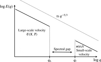
. This latter mimics small-scale turbulent fluctuations. The two components are assumed to be well separated in scale, i.e. if one Fourier transforms both components and looks at the corresponding energy spectra, the two sets of associated wavenumbers do not overlap (see figure 1 for a sketch). The scale separation is controlled by the dimensionless parameter
 ${\it\epsilon}=q_{L}/q_{l}$
. Large gaps thus correspond to small
 ${\it\epsilon}$
. A vanishing extension of the gap corresponds to
 ${\it\epsilon}=1$
. Our claim is that the scale separation in the velocity domain is also the scale separation one needs in the scalar dynamics for an eddy-diffusivity field to emerge. This claim was actually the main result of Mazzino (Reference Mazzino1997): by formal multiple-scale expansion, it has been shown that when the scalar dynamics reaches temporal/spatial scales of the order of those of
 $\boldsymbol{U}$
, an effective transport equation arises with a tensor eddy diffusivity. Note that we have introduced the concept of scale separation both in term of spatial scales and in term of temporal scales. This turns out to be possible in view of the fact that turbulence decay times are indeed related to spatial scales via sweeping effects (Kaneda, Ishihara & Gotoh Reference Kaneda, Ishihara and Gotoh1999).
Schematic representation of energy containing eddies in the presence of spectral gap separating the large-scale velocity component from the small-scale component. A Kolmogorov
 $q^{-5/3}$
spectral behaviour is assumed for the sake of example. Capital letters for spatial coordinates are used following the multiple-scale expansion jargon where they denote large scales.

In the multiple-scale expansion spirit, the large-scale character of
 $\boldsymbol{U}$
is encoded in its dependence on a new set of ‘slow’ variables
 $\boldsymbol{X}$
and
 $T$
. These latter are related to the usual set of ‘fast’ variables by
 $\boldsymbol{X}={\it\epsilon}\boldsymbol{x}$
and
 $T={\it\epsilon}^{2}t$
(Biferale et al.
Reference Biferale, Crisanti, Vergassola and Vulpiani1995) with the prescription to be treated as independent. The main aim is to determine the large-scale dynamics of
 ${\it\theta}$
on spatial/temporal scales comparable to those of
 $\boldsymbol{U}$
. We will denote by
 ${\it\Theta}$
this coarser scalar field and, following Mazzino et al. (Reference Mazzino, Musacchio and Vulpiani2005), we define its dynamics as ‘pre-asymptotic’ to distinguish it from the asymptotic transport which corresponds to the large-scale dynamics of
 ${\it\theta}$
on spatial/temporal scales much larger than those of
 $\boldsymbol{U}$
. This latter regime is diffusive and fully controlled by an eddy-diffusivity tensor (Biferale et al.
Reference Biferale, Crisanti, Vergassola and Vulpiani1995).
For the pre-asymptotic case, the main focus of the present paper, naive arguments would suggest a simple (wrong) conclusion:
 $\boldsymbol{U}$
gives the advection contribution in the large-scale equation for
 ${\it\theta}$
while (eddy) diffusion emerges from small-scale interactions between
 ${\it\theta}$
and
 $\boldsymbol{u}$
. A detailed analysis (Mazzino Reference Mazzino1997) actually shows that such a conclusion is doubly wrong: the large-scale velocity,
 $\boldsymbol{U}$
, is indeed not responsible for the sole large-scale advection, but it also enters into the renormalized diffusivity; the interaction between small scales gives rise not only to the expected eddy-diffusivity transport but also to an additional large-scale advection contribution.
In plain terms, the pre-asymptotic regime is fully described by the following equations:
 $$\begin{eqnarray}\partial _{t}{\it\Theta}+\boldsymbol{U}\boldsymbol{\cdot }\boldsymbol{\partial }{\it\Theta}=\partial _{i}(\unicode[STIX]{x1D60B}_{ij}\partial _{j}{\it\Theta})\end{eqnarray}$$
or, in equivalent form,
 $$\begin{eqnarray}\partial _{t}{\it\Theta}(\boldsymbol{x},t)+\boldsymbol{\partial }\boldsymbol{\cdot }(\boldsymbol{U}^{E}{\it\Theta})=\partial _{i}\partial _{j}(\unicode[STIX]{x1D60B}_{ij}^{E}{\it\Theta}),\end{eqnarray}$$
where
 ${\it\Theta}$
denotes the scalar field varying on pre-asymptotic scales and
 $$\begin{eqnarray}\displaystyle & U_{i}^{E}\equiv U_{i}+\partial _{j}\unicode[STIX]{x1D60B}_{ij} & \displaystyle\end{eqnarray}$$
 $$\begin{eqnarray}\displaystyle & \unicode[STIX]{x1D60B}_{ij}^{E}\equiv \displaystyle \frac{\unicode[STIX]{x1D60B}_{ij}+\unicode[STIX]{x1D60B}_{ji}}{2}. & \displaystyle\end{eqnarray}$$
The eddy diffusivity,
 $\unicode[STIX]{x1D60B}_{ij}(\boldsymbol{x},t)$
, is a tensor field in general neither symmetric nor positive definite. Its symmetric part (which is also positive definite) contributes to the diffusion process while both the symmetric and the antisymmetric parts enter, in general, into the effective advection velocity
 $\boldsymbol{U}^{E}$
which turns out to be compressible (scalar dynamics in compressible fields has been analysed, e.g. by Vergassola & Avellaneda (Reference Vergassola and Avellaneda1997) and Mauri (Reference Mauri2003)). The eddy diffusivity, often associated to the sole small-scale activity, here explicitly depends on the large-scale advection
 $\boldsymbol{U}$
. This fact causes the space–time dependence in the eddy diffusivity.
The Eulerian view for the large-scale dynamics given by (2.4) is equivalent to the Lagrangian Ito description:
 $$\begin{eqnarray}\frac{\text{d}\boldsymbol{x}(t)}{\text{d}t}=\boldsymbol{U}^{E}(\boldsymbol{x}(t),t)+{\bf\sigma}(\boldsymbol{x}(t),t)\boldsymbol{{\it\eta}}(t),\end{eqnarray}$$
where
 ${\bf\sigma}$
is the unique positive-definite solution of the matrix equation
 $\unicode[STIX]{x1D60B}_{ij}^{E}(\boldsymbol{x},t)=({\it\sigma}_{ip}(\boldsymbol{x},t){\it\sigma}_{jp}(\boldsymbol{x},t))/2$
. No explicit expression for
 $\unicode[STIX]{x1D60B}_{ij}(\boldsymbol{x},t)$
is available in general. A perturbative strategy has been carried out by Mazzino et al. (Reference Mazzino, Musacchio and Vulpiani2005) to obtain an approximate explicit expression for
 $\unicode[STIX]{x1D60B}_{ij}(\boldsymbol{x},t)$
in the limit of strong large-scale advection. The opposite limit has been analysed by Cencini et al. (Reference Cencini, Mazzino, Musacchio and Vulpiani2006).
The complexity of the problem is hidden inside the auxiliary equation through which
 $\unicode[STIX]{x1D60B}_{ij}^{E}(\boldsymbol{x},t)$
can be determined. The equation for the auxiliary field,
 ${\it\chi}$
, reads
 $$\begin{eqnarray}\partial _{t}{\it\chi}_{j}+(\boldsymbol{u}+\boldsymbol{U}(\boldsymbol{X},T))\boldsymbol{\cdot }\boldsymbol{\partial }{\it\chi}_{j}-D_{0}\partial ^{2}{\it\chi}_{j}=-u_{j},\end{eqnarray}$$
from which the expression for the eddy-diffusivity tensor follows:
 $$\begin{eqnarray}\unicode[STIX]{x1D60B}_{ij}(\boldsymbol{X},T)={\it\delta}_{ij}D_{0}-\langle u_{i}{\it\chi}_{j}\rangle .\end{eqnarray}$$
In (2.8) and (2.9), brackets denote averages on the small-scale statistics. An explicit, parametric dependence on slow variables does appear in the eddy diffusivity which becomes a large-scale varying field. To obtain the eddy-diffusivity tensor field, equation (2.8) must be solved for each value of the slow variables, thus making the problem highly complex and costly.
3 A simple model for the small-scale velocity fluctuations
As we have already emphasized in the last section, the exact results from the multiple-scale expansion leading to the expression for the eddy-diffusivity tensor field (2.9) are intrinsically formal. To obtain the eddy diffusivity one has indeed to know the small-scale velocity. Moreover, the space–time dependence of the eddy-diffusivity tensor implies that one has to numerically solve the auxiliary differential problem for all space and time collocation points. This is clearly a daunting task especially in relation to applications, e.g. related to the study of pollutant dispersion in the atmospheric environment.
To overcome these problems, our idea here is to build a stochastic model for small-scale velocity fluctuations mimicking relevant features of small-scale turbulence which, at the same time, allows one to obtain an explicit expression for the eddy-diffusivity tensor field. The statistical properties we require for our small-scale velocity field are: isotropy, stationarity, homogeneity and scale invariance of two-point statistics. This latter property is equivalent to imposing a power-law behaviour for the kinetic energy spectrum, e.g. à la Kolmogorov.
There are of course infinitely many possibilities to generate a stochastic field with the required statistical properties. Conversely, the requirement of having an explicit expression for the eddy-diffusivity tensor field leads to the exploitation of a specific class of velocity fields: the so-called parallel flows. Indeed, for parallel flows, in the auxiliary problem (2.8) the advective term disappears and explicit solutions can be obtained. By way of example, this class of flows was exploited by Mazzino & Vergassola (Reference Mazzino and Vergassola1997) to investigate interference phenomena in scalar transport.
Focusing henceforth on two dimensions, the stream function of our small-scale velocity field is sought as a superposition of
 $N$
independent spatial modes as
 $$\begin{eqnarray}{\it\Psi}(\boldsymbol{x},t;\boldsymbol{x}(0))=\mathop{\sum }_{i=1}^{N}\frac{A_{i}(\boldsymbol{x}(0),t)}{q_{i}}\sin [q_{i}\boldsymbol{n}(\boldsymbol{x}(0))\boldsymbol{\cdot }\boldsymbol{x}+{\it\theta}_{i}(\boldsymbol{x}(0))],\end{eqnarray}$$
where
 $\boldsymbol{x}$
is the spatial coordinate,
 $\boldsymbol{x}(0)$
is meant to stress that we choose independent randomly oriented parallel flows for each space location (in the following
 $\boldsymbol{x}(0)$
will be the initial conditions of Lagrangian particles through which we will investigate the transport problem; each
 $\boldsymbol{x}(0)$
will correspond to a given realization of the random process),
 $A_{i}(\boldsymbol{x}(0),t)$
and
 $q_{i}$
are the velocity amplitude and wavenumber modulus associated to the spatial mode
 $i$
. Finally,
 $\boldsymbol{n}(\boldsymbol{x}(0))$
is the direction angle associated to the initial condition
 $\boldsymbol{x}(0)$
and
 ${\it\theta}_{i}(\boldsymbol{x}(0))$
is the phase of the
 $i$
th mode. Direction angles and phases are random variables kept constant along each realization and uniformly distributed in
 $[0,2{\rm\pi})$
.
Following Lacorata, Mazzino & Rizza (Reference Lacorata, Mazzino and Rizza2008), where relative dispersion properties were analysed via a multiple-scale kinematic velocity field, we distribute spatial modes according to a given density factor (here
 $\sqrt{2}$
):
 $q_{i+1}=\sqrt{2}q_{i}$
. Wavelengths follow from the usual definition
 ${\it\lambda}_{i}=2{\rm\pi}/q_{i}$
. It has been shown by Boi, Afonso & Mazzino (Reference Boi, Afonso and Mazzino2015) that such a distribution guarantees a good description of the continuous limit
 $q_{i+1}-q_{i}\rightarrow 0$
.
To ensure a non-trivial temporal decay of two-point velocity statistics, velocity amplitudes can be generated via the Ornstein–Uhlenbeck process
 $$\begin{eqnarray}\frac{\text{d}A_{i}}{\text{d}t}=-\frac{A_{i}}{{\it\tau}_{i}}+\sqrt{\frac{2B_{i}}{{\it\tau}_{i}}}{\it\eta}_{i},\end{eqnarray}$$
where
 $\boldsymbol{{\it\eta}}$
is a zero-mean Gaussian white noise process with
 $\langle {\it\eta}_{i}(t){\it\eta}_{j}(t^{\prime })\rangle ={\it\delta}_{ij}{\it\delta}(t-t^{\prime })$
.
It is easy to verify from (3.2) that the following properties hold:
 $$\begin{eqnarray}\displaystyle \left.\begin{array}{@{}rcl@{}}\langle A_{i}(\boldsymbol{x}(0),t)\rangle \, & =\, & 0\\ \langle A_{i}^{2}(\boldsymbol{x}(0),t)\rangle \, & =\, & B_{i}\\ \langle A_{i}(\boldsymbol{x}(0),t)A_{i}(\boldsymbol{x}(0),t^{\prime })\rangle \, & =\, & B_{i}\exp \left(-\displaystyle \frac{|t-t^{\prime }|}{{\it\tau}_{i}}\right),\end{array}\right\} & & \displaystyle\end{eqnarray}$$
showing that the above process is thus stationary. From the numerical evidence reported by Kaneda et al. (Reference Kaneda, Ishihara and Gotoh1999), decorrelation times
 ${\it\tau}_{i}$
can be related to the large-scale sweeping via the simple relation
 ${\it\tau}_{i}={\it\alpha}/(\mathscr{U}_{rms}q_{i})$
where
 ${\it\alpha}$
is a free parameter (set equal to unity in the present study), and
 $\mathscr{U}_{rms}$
is the root mean square velocity.
From the stream function (3.1) the expression for the velocity field becomes a superposition of independent normal modes
 $\boldsymbol{u}=\sum _{i=1}^{N}\boldsymbol{u}_{i}$
. Namely,
 $$\begin{eqnarray}\displaystyle u_{1}\! & = & \displaystyle \!\mathop{\sum }_{i=1}^{N}A_{i}(\boldsymbol{x}(0),t)\sin [{\it\phi}(\boldsymbol{x}(0))]\cos \{q_{i}\cos [{\it\phi}(\boldsymbol{x}(0))]x+q_{i}\sin [{\it\phi}(\boldsymbol{x}(0))]y+{\it\theta}_{i}(\boldsymbol{x}(0))\}\nonumber\\ \displaystyle & & \displaystyle\end{eqnarray}$$
 $$\begin{eqnarray}\displaystyle u_{2}\! & = & \displaystyle \!-\mathop{\sum }_{i=1}^{N}A_{i}(\boldsymbol{x}(0),t)\cos [{\it\phi}(\boldsymbol{x}(0))]\cos \{q_{i}\cos [{\it\phi}(\boldsymbol{x}(0))]x+q_{i}\sin [{\it\phi}(\boldsymbol{x}(0))]y+{\it\theta}_{i}(\boldsymbol{x}(0))\},\nonumber\\ \displaystyle & & \displaystyle\end{eqnarray}$$
 ${\it\phi}(\boldsymbol{x}(0))$
is the angle between the
 $x$
-direction and the wavenumber direction. This latter is the same for each mode,
 $i$
, and only changes for different realizations. Note that because of the fact that the velocity field is generated along each particle path, there is thus for each value of the wavenumber modulus
 $q_{i}$
just one mode direction. However, because of the fact that each particle experiences independent random processes (in particular, different random angles,
 ${\it\phi}$
), the fact that we follow many particles to study the dispersion phenomenon actually implies that many directions for each value of
 $q_{i}$
are actually present, as in real turbulence.
Let us now show that our flow field is indeed homogeneous, isotropic and stationary. To do that, let us expand the velocity correlation function and exploit independence of random processes associated to different modes:
 $$\begin{eqnarray}\displaystyle \langle \boldsymbol{u}(\boldsymbol{x},t)\boldsymbol{\cdot }\boldsymbol{u}(\boldsymbol{x}^{\prime },t^{\prime })\rangle & = & \displaystyle \mathop{\sum }_{i=1}^{N}\langle A_{i}(\boldsymbol{x}(0),t)A_{i}(\boldsymbol{x}(0),t^{\prime })\rangle \nonumber\\ \displaystyle & & \displaystyle \times \,\langle \cos [q_{i}\boldsymbol{n}(\boldsymbol{x}(0))\boldsymbol{\cdot }\boldsymbol{x}+{\it\theta}_{i}(\boldsymbol{x}(0))]\cos [q_{i}\boldsymbol{n}(\boldsymbol{x}(0))\boldsymbol{\cdot }\boldsymbol{x}^{\prime }+{\it\theta}_{i}(\boldsymbol{x}(0))]\rangle .\nonumber\\ \displaystyle & & \displaystyle\end{eqnarray}$$
By means of well-known trigonometric identities, the above expression can be recast in the form
 $$\begin{eqnarray}\displaystyle \langle \boldsymbol{u}(\boldsymbol{x},t)\boldsymbol{\cdot }\boldsymbol{u}(\boldsymbol{x}^{\prime },t^{\prime })\rangle & = & \displaystyle \mathop{\sum }_{i=1}^{N}\frac{1}{2}\langle A_{i}(\boldsymbol{x}(0),t)A_{i}(\boldsymbol{x}(0),t^{\prime })\rangle \times \{\!\langle \!\cos [q_{i}\boldsymbol{n}(\boldsymbol{x}(0))\boldsymbol{\cdot }(\boldsymbol{x}+\boldsymbol{x}^{\prime })\nonumber\\ \displaystyle & & \displaystyle +\,2{\it\theta}_{i}(\boldsymbol{x}(0))]\!\rangle +\,\langle \cos [q_{i}\boldsymbol{n}(\boldsymbol{x}(0))\boldsymbol{\cdot }(\boldsymbol{x}-\boldsymbol{x}^{\prime })]\rangle \!\}.\end{eqnarray}$$
The phase average can be computed explicitly because phases are uniformly distributed:
 $$\begin{eqnarray}\displaystyle & & \displaystyle \langle \cos [q_{i}\boldsymbol{n}(\boldsymbol{x}(0))\boldsymbol{\cdot }(\boldsymbol{x}+\boldsymbol{x}^{\prime })+2{\it\theta}_{i}(\boldsymbol{x}(0))]\rangle \nonumber\\ \displaystyle & & \displaystyle \quad =\frac{1}{2{\rm\pi}}\int _{0}^{2{\rm\pi}}\,\text{d}{\it\theta}_{i}\cos [q_{i}\boldsymbol{n}(\boldsymbol{x}(0))\boldsymbol{\cdot }(\boldsymbol{x}+\boldsymbol{x}^{\prime })+2{\it\theta}_{i}]=0.\end{eqnarray}$$
Taking into account (3.3), we arrive at the final result:
 $$\begin{eqnarray}\langle \boldsymbol{u}(\boldsymbol{x},t)\boldsymbol{\cdot }\boldsymbol{u}(\boldsymbol{x}^{\prime },t^{\prime })\rangle =\mathop{\sum }_{i=1}^{N}\frac{B_{i}}{2}\exp \left(-\frac{|t-t^{\prime }|}{{\it\tau}_{i}}\right)\langle \cos [q_{i}\boldsymbol{n}(\boldsymbol{x}(0))\boldsymbol{\cdot }(\boldsymbol{x}-\boldsymbol{x}^{\prime })]\rangle ,\end{eqnarray}$$
from which stationarity and homogeneity clearly follow. Finally, the flow in (3.4a ) is also isotropic, due to our choice of considering randomly oriented uniformly distributed wavenumbers.
It now remains to choose
 $B_{i}$
in a way which enables us to obtain the desired kinetic energy spectrum. To do that, we recall the well-known definition of isotropic kinetic energy spectrum:
 $$\begin{eqnarray}E_{kin}\equiv \frac{1}{2}\langle |\boldsymbol{u}(\boldsymbol{x},t)|^{2}\rangle =\int _{0}^{\infty }\,\text{d}qE(q)\sim \mathop{\sum }_{i=1}^{N}E(q_{i}){\it\delta}q_{i},\end{eqnarray}$$
where
 ${\it\delta}q_{i}=q_{i+1}-q_{i}$
and the left-hand side of this relationship easily follows from (3.4a
):
 $$\begin{eqnarray}\frac{1}{2}\langle |\boldsymbol{u}(\boldsymbol{x},t)|^{2}\rangle =\mathop{\sum }_{i=1}^{N}\frac{\langle A_{i}^{2}\rangle }{4}=\mathop{\sum }_{i=1}^{N}\frac{B_{i}}{4}.\end{eqnarray}$$
By simple identification one ends up with
 $$\begin{eqnarray}E(q_{i}){\it\delta}q_{i}=\frac{1}{4}B_{i}\quad E_{kin}=\frac{1}{4}\mathop{\sum }_{i=1}^{N}B_{i}.\end{eqnarray}$$
In the specific case of a two-dimensional velocity field obeying, by way of example, the equivalent of the Kolmogorov 1941 theory,
 $E(q)=C{\it\varepsilon}^{2/3}q^{-5/3}$
(valid for two-dimensional turbulence in the inverse energy cascade (Boffetta & Ecke Reference Boffetta and Ecke2012)), where
 $C$
is the Kolmogorov constant and
 ${\it\varepsilon}$
denotes the energy dissipation rate, one has
 $B_{i}=4C{\it\varepsilon}^{2/3}q_{i}^{-5/3}{\it\delta}q_{i}$
. Different relationships can be trivially obtained by starting from different assumptions for the spectrum.
Assuming, as in figure 1, that small-scale turbulence is active for
 $q>q_{l}$
, one can simply express
 $C{\it\varepsilon}^{2/3}$
in terms of the turbulent kinetic energy
 $E_{kin}^{{>}}\equiv \int _{q_{l}}^{\infty }E(q)\,\text{d}q$
:
 $$\begin{eqnarray}C{\it\epsilon}^{2/3}={\textstyle \frac{2}{3}}E_{kin}^{{>}}q_{l}^{2/3}.\end{eqnarray}$$
Note that
 $E_{kin}^{{>}}$
is easily accessible in many CFD models (both RANS and LES) which use a closed equation for
 $E_{kin}^{{>}}$
to construct their closure models.
3.1 The model for the large-scale advection
To complete the definition of our flow model, the large-scale component,
 $\boldsymbol{U}$
, has to be defined. This latter is obtained in terms of the same model for the small-scale fluctuations except for the fact that we erase the dependence on
 $\boldsymbol{x}(0)$
in
 $A_{i}$
,
 ${\it\phi}_{i}$
and
 ${\it\theta}_{i}$
. This choice allows us to maintain an explicit dependence on large-scale space coordinates in the eddy-diffusivity tensor field. In plain words, we generate only one realization for each large-scale mode
 $i$
of the processes
 $A_{i}(t)$
,
 ${\it\phi}_{i}$
(here dependent on the
 $i$
th mode unlike what happens for the small-scale velocity component) and
 ${\it\theta}_{i}$
(here set to zero), which will be the same for every particle. The flow
 $\boldsymbol{U}$
is therefore
 $$\begin{eqnarray}\displaystyle \left.\begin{array}{@{}rcl@{}}U_{1}\, & =\, & \displaystyle U_{1}^{0}+\mathop{\sum }_{i=1}^{M}A_{i}(t)\sin ({\it\phi}_{i})\cos [q_{i}\cos ({\it\phi}_{i})x+q_{i}\sin ({\it\phi}_{i})y]\\ U_{2}\, & =\, & \displaystyle U_{2}^{0}-\mathop{\sum }_{i=1}^{M}A_{i}(t)\cos ({\it\phi}_{i})\cos [q_{i}\cos ({\it\phi}_{i})x+q_{i}\sin ({\it\phi}_{i})y],\end{array}\right\} & & \displaystyle\end{eqnarray}$$
where
 $M$
is the number of active wavenumbers
 $q_{i}$
with
 $q_{i}<q_{L}$
and
 $\boldsymbol{U}_{0}$
is the flow mean component. Note that the randomness of the direction angle
 ${\it\phi}_{i}$
guarantees that
 $\boldsymbol{U}-\boldsymbol{U}^{0}$
is zero-mean valued, since the flow is a
 $2{\rm\pi}$
-periodic function with respect to the angles, and
 $$\begin{eqnarray}\displaystyle & & \displaystyle \displaystyle \int _{0}^{{\rm\pi}}\,\text{d}{\it\phi}_{i}\sin ({\it\phi}_{i})\cos [q_{i}\cos ({\it\phi}_{i})x+q_{i}\sin ({\it\phi}_{i})y]\nonumber\\ \displaystyle & & \displaystyle \quad +\,\int _{{\rm\pi}}^{2{\rm\pi}}\,\text{d}{\it\phi}_{i}\sin ({\it\phi}_{i})\cos [q_{i}\cos ({\it\phi}_{i})x+q_{i}\sin ({\it\phi}_{i})y]=0,\end{eqnarray}$$
 $$\begin{eqnarray}\displaystyle & & \displaystyle \displaystyle \int _{0}^{{\rm\pi}}\,\text{d}{\it\phi}_{i}\cos ({\it\phi}_{i})\cos [q_{i}\cos ({\it\phi}_{i})x+q_{i}\sin ({\it\phi}_{i})y]\nonumber\\ \displaystyle & & \displaystyle \quad +\,\int _{{\rm\pi}}^{2{\rm\pi}}\,\text{d}{\it\phi}_{i}\cos ({\it\phi}_{i})\cos [q_{i}\cos ({\it\phi}_{i})x+q_{i}\sin ({\it\phi}_{i})y]=0,\end{eqnarray}$$
having done the substitution
 ${\it\phi}\rightarrow {\it\phi}-{\rm\pi}$
in the two integrals from
 ${\rm\pi}$
to
 $2{\rm\pi}$
.
To conclude this section, let us make a comment on
 $\mathscr{U}_{rms}$
. The total kinetic energy is obtained by averaging on both the small and large scales. We will keep the bracket notation for the small-scale ensemble mean value, whereas we will use an overline to indicate the large-scale mean value, which we can obtain by means of a space–time average (ergodicity hypothesis), recalling that the amplitude processes are realizations of (3.2) and then they fulfil (3.3). The result is easily obtained as follows:
 $$\begin{eqnarray}\displaystyle E_{kin} & = & \displaystyle \frac{1}{2}\overline{\langle (\boldsymbol{u}+\boldsymbol{U})\boldsymbol{\cdot }(\boldsymbol{u}+\boldsymbol{U})\rangle }\nonumber\\ \displaystyle & = & \displaystyle \frac{1}{2}\mathop{\sum }_{i,j=1}^{N}\langle \boldsymbol{u}_{i}\boldsymbol{\cdot }\boldsymbol{u}_{j}\rangle +\frac{1}{2}\mathop{\sum }_{i,j=1}^{M}\overline{\boldsymbol{U}_{i}\boldsymbol{\cdot }\boldsymbol{U}_{j}}+\frac{1}{2}|\boldsymbol{U}^{0}|^{2}=E_{kin}^{{>}}+E_{kin}^{{<}},\end{eqnarray}$$
which follows from the fact that amplitudes of different modes are uncorrelated and where we have defined
 $$\begin{eqnarray}E_{kin}^{{<}}=\frac{|\boldsymbol{U}^{0}|^{2}}{2}+\mathop{\sum }_{i=1}^{M}\frac{B_{i}}{4}.\end{eqnarray}$$
It then follows that the velocity root mean square reads
 $$\begin{eqnarray}\mathscr{U}_{rms}\equiv \sqrt{2E_{kin}}=\sqrt{2(E_{kin}^{{<}}+E_{kin}^{{>}})}.\end{eqnarray}$$
The fact that
 $\boldsymbol{U}^{0}$
explicitly enters in
 $\mathscr{U}_{rms}$
, thus acting as a sweeping effect in the same ways as large eddies do, is a consequence of our choice not to assume Galilean invariance. This latter symmetry is indeed often broken in the presence of realistic boundary conditions, e.g. those encountered in environmental problems.
4 Explicit expression for the eddy-diffusivity field
To obtain the eddy-diffusivity field associated to the flow field defined in § 3, one can proceed along two different paths. One is based on the Eulerian view and follows from the application of (2.9). The second possibility is to start from the definition of eddy diffusivity in Lagrangian terms and proceed with the calculation in this framework. We decided to follow the second option and we provide here some details of the calculation which, at the very end, will lead to an explicit expression for both the eddy-diffusivity tensor and the effective large-scale advection defined in (2.5).
The starting point is the well-known definition of eddy diffusivity in Lagrangian terms:
 $$\begin{eqnarray}\unicode[STIX]{x1D60B}_{{\it\alpha}{\it\beta}}(\boldsymbol{U})=\lim _{t\rightarrow \infty }\frac{1}{2}\frac{\text{d}}{\text{d}t}\langle (x_{{\it\alpha}}(t)-\langle x_{{\it\alpha}}(t)\rangle )(x_{{\it\beta}}(t)-\langle x_{{\it\beta}}(t)\rangle )\rangle ,\end{eqnarray}$$
where brackets denote averages with respect to the random small-scale velocity statistics and
 $x_{{\it\alpha}}(t)$
defines a particle trajectory ruled by the Langevin equation
 $$\begin{eqnarray}\frac{\text{d}\boldsymbol{x}(t)}{\text{d}t}=\boldsymbol{U}(\boldsymbol{X}(T),T)+\boldsymbol{u}(\boldsymbol{x}(t),t).\end{eqnarray}$$
From now on we neglect the molecular diffusivity, as customary when studying transport in turbulent (chaotic) environments, and adopt the convention that Greek indexes are used for vector components while Latin indexes select different normal modes. As already stated, capital letters for spatial coordinates originate from the multiple-scale jargon and are meant to stress that
 $\boldsymbol{U}(\boldsymbol{X},T)$
evolve on scales much larger than those of
 $\boldsymbol{u}$
. The space–time dependence in
 $\boldsymbol{U}(\boldsymbol{X},T)$
will thus be considered as parametric. Physically, this amounts to saying that in the transport process, particles see a constant large-scale advection for the entire duration of the renormalization stage associated to the small-scale dynamics.
Because of the fact that the spatial modes involved in (3.4a ) are mutually uncorrelated and statistically homogeneous, we can proceed by analysing the transport process for each single mode and then adding all contributions. This interesting result is reported in appendix A.
The starting point is to rotate coordinates in a manner such that the wavenumber is aligned with the
 $x$
-axis. This is easily done in terms of suitable rotation matrices
 $\unicode[STIX]{x1D619}_{{\it\alpha}{\it\beta}}({\it\phi}(\boldsymbol{x}(0)))$
,
 $x_{{\it\alpha}}^{\prime }=\unicode[STIX]{x1D619}_{{\it\alpha}{\it\beta}}({\it\phi}(\boldsymbol{x}(0)))x_{{\it\beta}}$
with an angle such that in the new coordinate system
 $\boldsymbol{n}^{\prime }=\boldsymbol{R}\boldsymbol{n}=(1,0)$
. Recalling that for a matrix belonging to the rotation group in two dimensions,
 $\text{SO}(2,\mathbb{R})$
, one has
 $\unicode[STIX]{x1D619}_{11}=\unicode[STIX]{x1D619}_{22}$
and
 $\unicode[STIX]{x1D619}_{12}=-\unicode[STIX]{x1D619}_{21}$
, the expression for the velocity field in the rotated system is easily obtained:
 $$\begin{eqnarray}\displaystyle \left.\begin{array}{@{}c@{}}u_{i\,1}^{\prime }(x^{\prime },y^{\prime },t)=0\\ u_{i\,2}^{\prime }(x^{\prime },y^{\prime },t)=-A_{i}(\boldsymbol{x}^{\prime }(0),t)\cos [q_{i}x^{\prime }+{\it\theta}_{i}(\boldsymbol{x}(0))].\end{array}\right\} & & \displaystyle\end{eqnarray}$$
For each normal mode
 $\boldsymbol{u}_{i}^{\prime }$
, in its new reference frame, the equation of motion turns out to be (omitting for the sake of brevity dependence on large-scale variables in
 $\boldsymbol{U}^{\prime }$
)
 $$\begin{eqnarray}\frac{\text{d}x_{i}^{\prime }}{\text{d}t}=\boldsymbol{u}_{i}^{\prime }(\boldsymbol{x}_{i}^{\prime }(t),t)+\boldsymbol{U}^{\prime },\end{eqnarray}$$
where
 $\boldsymbol{U}^{\prime }=\boldsymbol{R}\boldsymbol{U}$
. Thus the solution for the
 $i$
th mode is
 $$\begin{eqnarray}\displaystyle \left.\begin{array}{@{}c@{}}x_{i}^{\prime }=x^{\prime }(0)+U_{1}^{\prime }t\\ y_{i}^{\prime }=y^{\prime }(0)+U_{2}^{\prime }t-\displaystyle \int _{0}^{t}\,\text{d}t^{\prime }A_{i}(\boldsymbol{x}^{\prime }(0),t^{\prime })\cos [q_{i}(x^{\prime }(0)+U_{1}^{\prime }t^{\prime })+{\it\theta}_{i}(\boldsymbol{x}(0))].\end{array}\right\} & & \displaystyle\end{eqnarray}$$
Straightforwardly, only
 $D_{i\,22}\equiv \langle (y_{i}^{\prime }(t)-\langle y_{i}^{\prime }(t)\rangle )^{2}\rangle$
is non-zero in this new coordinate system. From (3.3), it follows that
 $$\begin{eqnarray}\langle y_{i}^{\prime }\rangle =y^{\prime }(0)+U_{2}^{\prime }t.\end{eqnarray}$$
Exploiting well-known trigonometric identities, the expression for
 $D_{i\,22}$
reads
 $$\begin{eqnarray}\displaystyle D_{i\,22} & = & \displaystyle \frac{1}{4}\frac{\text{d}}{\text{d}t}\int _{0}^{t}\,\text{d}t^{\prime }\int _{0}^{t}\,\text{d}t^{\prime \prime }\langle A_{i}(t^{\prime })A_{i}(t^{\prime \prime })\rangle \langle \!\cos [q_{i}U_{1}^{\prime }(t^{\prime }-t^{\prime \prime })]\nonumber\\ \displaystyle & & \displaystyle +\,\cos [q_{i}(2x^{\prime }(0)+U_{1}^{\prime }(t^{\prime }+t^{\prime \prime }))+2{\it\theta}_{i}]\!\rangle ,\end{eqnarray}$$
where we have exploited the fact that
 $A_{i}$
and
 ${\it\theta}_{i}$
are independent random processes together with the properties given by (3.3).
The phase average inside the above integral can be computed explicitly because phases are uniformly distributed:
 $$\begin{eqnarray}\displaystyle & & \displaystyle \langle \cos [q_{i}(2x^{\prime }(0)+U_{1}^{\prime }(t^{\prime }+t^{\prime \prime }))+2{\it\theta}_{i}]\rangle \nonumber\\ \displaystyle & & \displaystyle \quad =\frac{1}{2{\rm\pi}}\int _{0}^{2{\rm\pi}}\,\text{d}{\it\theta}_{i}\cos [q_{i}(2x^{\prime }(0)+U_{1}^{\prime }(t^{\prime }+t^{\prime \prime }))+2{\it\theta}_{i}]=0,\end{eqnarray}$$
from which, after simple manipulation and exploiting again (3.3), expression (4.7) becomes
 $$\begin{eqnarray}\displaystyle D_{i\,22}^{\prime }=\lim _{t\rightarrow \infty }\int _{0}^{t}\,\text{d}t^{\prime }B_{i}\frac{\exp \left(\displaystyle -\frac{|t^{\prime }-t|}{{\it\tau}_{i}}\right)}{2}\cos [q_{i}U_{1}^{\prime }(t^{\prime }-t)]=\frac{B_{i}}{2}\frac{{\it\tau}_{i}}{{\it\tau}_{i}^{2}q_{i}^{2}{U_{1}^{\prime }}^{2}+1}. & & \displaystyle\end{eqnarray}$$
The effect of the large-scale velocity at the denominator always causes a reduction of the eddy diffusivity.
The last step is to go back to the original coordinate system for each normal mode remembering that
 $\boldsymbol{n}^{\prime }=(1,0)$
and thus
 $U_{1}=\boldsymbol{n}^{\prime }\boldsymbol{\cdot }\boldsymbol{U}^{\prime }=\boldsymbol{n}\boldsymbol{\cdot }\boldsymbol{U}$
. We also have to sum all contributions coming from different modes
 $i$
(see again appendix A) and average over the angular directions:
 $$\begin{eqnarray}\displaystyle \left.\begin{array}{@{}rcl@{}}\unicode[STIX]{x1D60B}_{11}\, & =\, & \displaystyle \mathop{\sum }_{i=1}^{N}\langle D_{i\,22}^{\prime }\unicode[STIX]{x1D619}_{21}^{2}\rangle =\mathop{\sum }_{i=1}^{N}\frac{B_{i}}{2}\left\langle \frac{{\it\tau}_{i}\sin ^{2}[{\it\phi}]}{{\it\tau}_{i}^{2}q_{i}^{2}(\boldsymbol{n}({\it\phi})\boldsymbol{\cdot }\boldsymbol{U})^{2}+1}\right\rangle \\ \unicode[STIX]{x1D60B}_{12}\, & =\, & \displaystyle \mathop{\sum }_{i=1}^{N}\langle D_{i\,22}^{\prime }\unicode[STIX]{x1D619}_{21}\unicode[STIX]{x1D619}_{11}\rangle =-\mathop{\sum }_{i=1}^{N}\frac{B_{i}}{2}\left\langle \frac{{\it\tau}_{i}\sin [{\it\phi}]\cos [{\it\phi}]}{{\it\tau}_{i}^{2}q_{i}^{2}(\boldsymbol{n}({\it\phi})\boldsymbol{\cdot }\boldsymbol{U})^{2}+1}\right\rangle \\ \unicode[STIX]{x1D60B}_{22}\, & =\, & \displaystyle \mathop{\sum }_{i=1}^{N}\langle D_{i\,22}^{\prime }\unicode[STIX]{x1D619}_{22}^{2}\rangle =\mathop{\sum }_{i=1}^{N}\frac{B_{i}}{2}\left\langle \frac{{\it\tau}_{i}\cos ^{2}[{\it\phi}]}{{\it\tau}_{i}^{2}q_{i}^{2}(\boldsymbol{n}({\it\phi})\boldsymbol{\cdot }\boldsymbol{U})^{2}+1}\right\rangle .\end{array}\right\} & & \displaystyle\end{eqnarray}$$
It is worth recalling that
 $\unicode[STIX]{x1D60B}_{12}=\unicode[STIX]{x1D60B}_{21}$
since
 $\unicode[STIX]{x1D619}_{22}=\unicode[STIX]{x1D619}_{11}$
. Eventually, the angular averages give rise to the following three integrals:
 $$\begin{eqnarray}\displaystyle \left.\begin{array}{@{}c@{}}\displaystyle \int _{0}^{2{\rm\pi}}\frac{\sin ^{2}{\it\phi}\,\text{d}{\it\phi}}{{\it\tau}_{i}^{2}q_{i}^{2}(U_{1}\cos {\it\phi}+U_{2}\sin {\it\phi})^{2}+1}\\ \displaystyle -\int _{0}^{2{\rm\pi}}\frac{\sin {\it\phi}\cos {\it\phi}\,\text{d}{\it\phi}_{i}}{{\it\tau}_{i}^{2}q_{i}^{2}(U_{1}\cos {\it\phi}+U_{2}\sin {\it\phi})^{2}+1}\\ \displaystyle \int _{0}^{2{\rm\pi}}\frac{\cos ^{2}{\it\phi}\,\text{d}{\it\phi}}{{\it\tau}_{i}^{2}q_{i}^{2}(U_{1}\cos {\it\phi}+U_{2}\sin {\it\phi})^{2}+1}.\end{array}\right\} & & \displaystyle\end{eqnarray}$$
The three integrals involved in the above expressions can be evaluated exactly. This is the very last step to obtain the explicit expression of the eddy-diffusivity field. The final result reads
 $$\begin{eqnarray}\displaystyle \unicode[STIX]{x1D60B}_{11} & = & \displaystyle \frac{\mathscr{U}_{rms}^{2}}{{\it\alpha}^{2}}\left[\frac{{\it\alpha}^{2}}{\mathscr{U}_{rms}^{2}}U_{1}^{2}(U_{2}^{2}+U_{1}^{2})+(U_{2}^{2}-U_{1}^{2})\sqrt{\frac{{\it\alpha}^{2}}{\mathscr{U}_{rms}^{2}}(U_{1}^{2}+U_{2}^{2})+1}+U_{1}^{2}-U_{2}^{2}\right]\nonumber\\ \displaystyle & & \displaystyle \times \,\left[\sqrt{\frac{{\it\alpha}^{2}}{\mathscr{U}_{rms}^{2}}(U_{1}^{2}+U_{2}^{2})+1}(U_{1}^{2}+U_{2}^{2})^{2}\right]^{-1}\mathop{\sum }_{i=1}^{N}\frac{B_{i}}{2}{\it\tau}_{i}\end{eqnarray}$$
 $$\begin{eqnarray}\displaystyle \unicode[STIX]{x1D60B}_{22} & = & \displaystyle \frac{\mathscr{U}_{rms}^{2}}{{\it\alpha}^{2}}\left[\frac{{\it\alpha}^{2}}{\mathscr{U}_{rms}^{2}}U_{2}^{2}(U_{2}^{2}+U_{1}^{2})+(U_{1}^{2}-U_{2}^{2})\sqrt{\frac{{\it\alpha}^{2}}{\mathscr{U}_{rms}^{2}}(U_{1}^{2}+U_{2}^{2})+1}+U_{2}^{2}-U_{1}^{2}\right]\nonumber\\ \displaystyle & & \displaystyle \times \,\left[\sqrt{\frac{{\it\alpha}^{2}}{\mathscr{U}_{rms}^{2}}(U_{1}^{2}+U_{2}^{2})+1}(U_{1}^{2}+U_{2}^{2})^{2}\right]^{-1}\mathop{\sum }_{i=1}^{N}\frac{B_{i}}{2}{\it\tau}_{i}\end{eqnarray}$$
 $$\begin{eqnarray}\displaystyle \unicode[STIX]{x1D60B}_{12} & = & \displaystyle \frac{\mathscr{U}_{rms}^{2}}{{\it\alpha}^{2}}U_{2}U_{1}\left[\frac{{\it\alpha}^{2}}{\mathscr{U}_{rms}^{2}}(U_{2}^{2}+U_{1}^{2})-2\sqrt{\frac{{\it\alpha}^{2}}{\mathscr{U}_{rms}^{2}}(U_{1}^{2}+U_{2}^{2})+1}+2\right]\nonumber\\ \displaystyle & & \displaystyle \times \,\left[\sqrt{\frac{{\it\alpha}^{2}}{\mathscr{U}_{rms}^{2}}(U_{1}^{2}+U_{2}^{2})+1}(U_{1}^{2}+U_{2}^{2})^{2}\right]^{-1}\mathop{\sum }_{i=1}^{N}\frac{B_{i}}{2}{\it\tau}_{i}.\end{eqnarray}$$
In tensorial form, the above expressions can be written as
 $$\begin{eqnarray}\displaystyle D_{{\it\beta}{\it\gamma}} & = & \displaystyle \frac{\displaystyle \frac{\mathscr{U}_{rms}^{2}}{{\it\alpha}^{2}}\left[\displaystyle \frac{{\it\alpha}^{2}}{\mathscr{U}_{rms}^{2}}|\boldsymbol{U}|^{2}U_{{\it\beta}}U_{{\it\gamma}}+(|\boldsymbol{U}|^{2}\,{\it\delta}_{{\it\beta}{\it\gamma}}-2U_{{\it\beta}}U_{{\it\gamma}})\left(\displaystyle \sqrt{\frac{{\it\alpha}^{2}}{\mathscr{U}_{rms}^{2}}|\boldsymbol{U}|^{2}+1}-1\right)\right]}{\sqrt{\displaystyle \frac{{\it\alpha}^{2}}{\mathscr{U}_{rms}^{2}}|\boldsymbol{U}|^{2}+1}\;|\boldsymbol{U}|^{4}}\nonumber\\ \displaystyle & & \displaystyle \times \,\mathop{\sum }_{i=1}^{N}\frac{B_{i}}{2}{\it\tau}_{i},\end{eqnarray}$$
where it is now evident how the effect of the large-scale velocity acts to renormalize the bare correlation time.
Note that in the limit
 $\boldsymbol{U}\rightarrow 0$
one obtains the ‘bare’ diffusivity whose entries are
 $\unicode[STIX]{x1D60B}_{11}=\unicode[STIX]{x1D60B}_{22}=\sum _{i=1}^{N}(B_{i}{\it\tau}_{i}/4)$
and
 $\unicode[STIX]{x1D60B}_{12}=0$
.
To conclude this section it is worth remarking that expressions similar to (4.15) can also be derived in three dimensions. Their final form, together with a sketch of the derivation, is reported in appendix C.
4.1 The effective advecting velocity
To determine the effective advection field (2.5) one has to take the divergence of
 $\unicode[STIX]{x1D60B}_{{\it\alpha}{\it\beta}}$
from the explicit expressions (4.12)–(4.14). This can be easily done via a chain rule for the derivatives, once returned to the original variables
 $\boldsymbol{x},t$
.
Recalling that
 $\unicode[STIX]{x1D60B}_{{\it\alpha}{\it\beta}}=\sum _{p=1}^{N}D_{p\,{\it\alpha}{\it\beta}}$
, one arrives at
 $$\begin{eqnarray}\frac{\partial \unicode[STIX]{x1D60B}_{{\it\alpha}{\it\beta}}}{\partial x_{{\it\beta}}}=\mathop{\sum }_{p=1}^{N}\frac{\partial D_{p\,{\it\alpha}{\it\beta}}}{\partial U_{{\it\gamma}}}\frac{\partial U_{{\it\gamma}}}{\partial x_{{\it\beta}}}.\end{eqnarray}$$
The resulting expressions for
 $\partial D_{p\,{\it\alpha}{\it\beta}}/\partial U_{{\it\gamma}}$
are reported in appendix B together with the velocity gradient tensor.
5 Numerical study
The main aim of this section is to verify the reliability of our expressions for the eddy diffusivity and effective advection by varying the extension of the spectral gap depicted in figure 1. The limiting case will be a situation where the spectral gap reduces to zero, as in many situations of interest. As a further objective, in the absence of a spectral gap, we will perform a comparison between our models performance and other possible simpler choices to describe the effect of the unresolved small-scale motion.
For these purposes we perform kinematic simulations mimicking homogeneous, isotropic and stationary turbulence in two dimensions accompanied by Lagrangian simulations. Kinematic simulations are a widely used tool to investigate turbulent dispersion both from the point of view of relative dispersion and of absolute dispersion. Interested readers can refer, by way of example, to Crisanti et al. (Reference Crisanti, Falcioni, Paladin and Vulpiani1991) and Fung et al. (Reference Fung, Hunt, Malik and Perkins1992), and references therein.
Once fully resolved flow fields are available, it is easy to isolate their large-scale components
 $\boldsymbol{U}$
(i.e. active for
 $q<q_{L}$
) and small-scale components
 $\boldsymbol{u}$
(i.e. active for
 $q>q_{l}$
). The extension of the spectral gap will be a free parameter. In the following we will set
 ${\it\varepsilon}=1$
and
 $q_{l}=2{\rm\pi}$
which fix the dimensionless form of our model.
The total field
 $\boldsymbol{U}+\boldsymbol{u}$
we obtain in this way will be the background in which a puff of
 $\mathscr{N}$
seeded particles will evolve according to the Langevin equation (2.2).
The evolution given by (2.2) in terms of the fully resolved velocity field is what we can define as our ‘exact’ evolution. One the other hand, retaining the sole large-scale flow component
 $\boldsymbol{U}$
, we can easily calculate the eddy-diffusivity field and the effective advection. Through these fields the evolution equation of the same initial puff of seeded particles can be determined via (2.7) and properly compared with the ‘exact’ puff evolution.
For testing purposes, let us start by considering the simpler situation where the velocity field is of the form
 $\boldsymbol{U}+\boldsymbol{u}$
with
 $\boldsymbol{U}$
constant in space and time and
 $\boldsymbol{u}$
built in terms of
 $N=5$
modes in (3.4a
) for
 $q>q_{l}$
. For
 $i=1,\ldots ,5$
we assume
 $B_{i}=4C{\it\varepsilon}^{2/3}q_{i}^{-5/3}$
, with
 $C=1.4$
(remember that
 ${\it\varepsilon}=1$
and
 $q_{l}=2{\rm\pi}$
). Here
 $\boldsymbol{U}$
is
 $(20,3)$
and
 $\mathscr{U}_{rms}\sim 20.3$
. This means that the maximum and minimum decay times of the small-scale modes are
 ${\it\tau}_{max}\sim 0.008$
and
 ${\it\tau}_{min}\sim 0.002$
, respectively. Because of the fact that no large-scale velocity component is present here (we only have the mean field component), a pure diffusive regime is expected for times sufficiently larger than
 ${\it\tau}_{max}\sim 0.008$
. The expression for the eddy-diffusivity tensor follow from (4.12)–(4.14) from which we have:
 $\langle (x_{{\it\alpha}}-\langle x_{{\it\alpha}}\rangle )(x_{{\it\beta}}-\langle x_{{\it\beta}}\rangle )\rangle =2\unicode[STIX]{x1D60B}_{{\it\alpha}{\it\beta}}t$
, with
 $\unicode[STIX]{x1D60B}_{11}=0.0051$
,
 $\unicode[STIX]{x1D60B}_{22}=0.0037$
,
 $\unicode[STIX]{x1D60B}_{12}=0.00022$
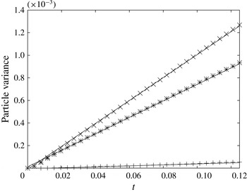
. The numerical results obtained from the integration of the Langevin equation with the fully resolved velocity field are shown in figure 2. Averages are performed by following
 $9\times 10^{4}$
particles and their initial positions are uniformly spread on a unit square. The resulting time behaviour of
 $\langle (x_{{\it\alpha}}-\langle x_{{\it\alpha}}\rangle )(x_{{\it\beta}}-\langle x_{{\it\beta}}\rangle )\rangle$
from the numerical integration of the Langevin equation is fitted with the function
 $at+b$
for
 $t>{\it\tau}_{max}$
. The best fit curves agree with our model predictions with relative errors of
 ${\sim}2\,\%$
(for
 $\unicode[STIX]{x1D60B}_{11}$
), 1 % (for
 $\unicode[STIX]{x1D60B}_{22}$
) and 8 % (for
 $\unicode[STIX]{x1D60B}_{12}$
).
Particle variance
 ${\it\zeta}_{{\it\alpha}{\it\beta}}=\langle (x_{{\it\alpha}}-\langle x_{{\it\alpha}}\rangle )(x_{{\it\beta}}-\langle x_{{\it\beta}}\rangle )\rangle$
versus time in a small-scale flow plus a constant component. Continuous lines represent the theoretical slopes; symbols represent the numerical results for
 ${\it\zeta}_{11}$
(
 $\times$
),
 ${\it\zeta}_{12}$
(
 $+$
), and
 ${\it\zeta}_{22}$
(
 $\ast$
).

5.1 Observables to measure model reliability
Let us now pass to analyse the general situation in the presence of a large-scale velocity component. A possible way to assess the performances of our eddy diffusivity and effective advection model for the evolution of a puff of initially seeded particles is to compare (against the ‘exact’ evolution) different absolute dispersion observables associated to the puff as a function of time. Here we focus on different moments of particle displacements from their initial positions in the frame of reference moving with the mean flow
 $\boldsymbol{U}^{0}$
. In formulae, we will compute
 $$\begin{eqnarray}M_{p}(t)=\langle |\boldsymbol{x}-\boldsymbol{x}(0)-\boldsymbol{U}^{0}t|^{p}\rangle\end{eqnarray}$$
for different
 $p$
. Another observable we will consider is the probability density function,
 $P$
, of
 ${\rm\Delta}(t)\equiv |\boldsymbol{x}-\boldsymbol{x}(0)-\boldsymbol{U}^{0}t|$
at different times. This latter quantity encodes both large and small fluctuations of particle displacements thus giving a complete description of the absolute dispersion phenomenon.
5.2 Results and discussion
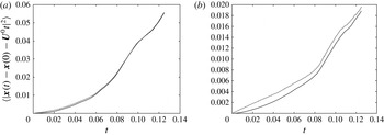
Let us start to investigate the reliability of our closure model based on the eddy-diffusivity tensor field (4.12)–(4.14) and effective advection (4.16) by varying the extension of the spectral gap depicted in figure 1. In figure 3 we report the moment
 $M_{2}(t)$
defined by (5.1) for the ‘exact’ evolution (continuous line) and for our closure model (dotted line) for
 ${\it\epsilon}=q_{L}/q_{l}=1$
(b), corresponding to the absence of spectral gap, and
 ${\it\epsilon}=0.125$
, (a). The small-scale field has
 $N=14$
modes, while the large-scale component has one active mode (i.e.
 $M=1$
). The mean field component is
 $\boldsymbol{U}^{0}=(4,0)$
.
As one can see from figure 3, the two descriptions are almost indistinguishable already for
 ${\it\epsilon}=0.125$
. For
 ${\it\epsilon}=1$
our closure works reasonably well and captures the relevant feature of the exact curve. Note that at the final observation time the mean particle displacement is of order one and thus comparable to
 $2{\rm\pi}/q_{L}=1$
(case corresponding to
 ${\it\epsilon}=1$
) and smaller than
 $2{\rm\pi}/q_{L}=8$
(case corresponding to
 ${\it\epsilon}=0.125$
). This tells us that we are observing the dispersion phenomenon in the pre-asymptotic regime. In terms of typical times, the largest small-scale velocity correlation time
 ${\it\tau}_{max}\sim 0.035$
is four times smaller than the observation time
 $t=0.125$
which also justifies a description based on the eddy diffusivity.
Plots of
 $M_{2}$
versus time, following the exact evolution (continuous line) and our description with eddy diffusivity plus effective velocity (dotted line): (a)
 ${\it\epsilon}=0.125$
, and
 $\mathscr{U}_{rms}=4.8$
; (b)
 ${\it\epsilon}=1$
and
 $\mathscr{U}_{rms}=4.5$
.

To quantitatively estimate the discrepancy between the two descriptions we have computed the relative errors for different values of
 ${\it\epsilon}$
. Errors have been defined in terms of the
 $L^{2}$
-norm
 $\Vert \,f\Vert _{L^{2}}^{2}\equiv \int \,\text{d}t|\,f(t)|^{2}$
from which the relative error follows from the definition of relative functional distance:
 $$\begin{eqnarray}D_{p}({\it\epsilon})\equiv \frac{\Vert M_{p}({\it\epsilon})-M_{p}^{E}({\it\epsilon})\Vert _{L^{2}}^{2}}{\Vert M_{p}({\it\epsilon})\Vert _{L^{2}}\Vert M_{p}^{E}({\it\epsilon})\Vert _{L^{2}}}.\end{eqnarray}$$
In this expression
 $M_{p}^{E}({\it\epsilon})$
refers to the exact evolution while
 $M_{p}({\it\epsilon})$
corresponds to our closure.
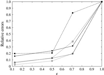
The results are summarized in figure 4 where
 $D_{p}({\it\epsilon})/D_{p}(1)$
is shown for different values of
 ${\it\epsilon}$
. As expected, the smallest errors are for
 $p=2$
corresponding to the errors calculated on second-order moments. It is interesting to remark that also
 $p\neq 2$
provide satisfactory results. This is probably related to the quasi-Gaussian character of the dispersion process on pre-asymptotic scales.
The
 $L^{2}$
-relative errors
 $D_{p}({\it\epsilon})/D_{p}(1)$
(see text) for different orders of the moment
 $p$
as a function of the gap extension
 ${\it\epsilon}$
. Full circles refer to
 $p=1/2$
,
 $\times$
to
 $p=1$
, empty circles to
 $p=2$
, empty squares to
 $p=3$
, and full squares to
 $p=4$
. Here
 $\mathscr{U}_{rms}=4.5$
. The normalizing factors
 $D_{p}(1)$
are:
 $D_{1/2}(1)=0.34$
,
 $D_{1}(1)=0.12$
,
 $D_{2}(1)=0.019$
,
 $D_{3}(1)=0.0035$
,
 $D_{4}(1)=0.00072$
.

Plots of
 $M_{2}$
(a) and
 $M_{4}$
(b) versus time for
 ${\it\epsilon}=1$
and
 $\mathscr{U}_{rms}=4.5$
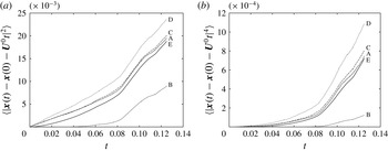
. The continuous line depicts the exact evolution, and it is indicated by the letter E; case A is our closure; case B is the evolution with large-scale flow only; case C represents our closure without the effective compressible velocity contribution; the ‘naive’ description is finally indicated by letter D.

Having shown that our closure model works even in the absence of scale separation within the pre-asymptotic stage of the dispersion phenomenon, we are now ready to investigate how our closure compares with alternative strategies. We decided to choose as reference closures the following cases: case A, our closure; case B, evolution with the sole large-scale velocity (i.e. no closure at all); case C, our closure without the effective (compressible) large-scale advection; case D, a naive closure based on the idea that the eddy diffusivity only depends on the small-scale advection. Accordingly, in this latter case the eddy diffusivity is obtained by setting to zero the large-scale velocity component (including the mean field component). All cases have
 $\mathscr{U}_{rms}\sim 4.5$
.
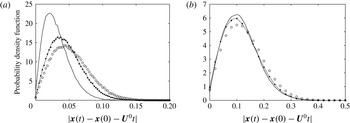
The results are reported in figures 5 and 6. In figure 5 we show the behaviour of the moments
 $M_{2}(t)$
(a) and
 $M_{4}(t)$
(b) as a function of time for the ‘exact’ evolution (continuous line), which we indicate with the letter E, and for cases A, B, C and D, with
 ${\it\epsilon}=1$
. In figure 6,
 $P({\rm\Delta}(t))$
is shown for
 $t=0.0325$
(corresponding to
 $t\sim {\it\tau}_{max}$
) and
 $t=0.125$
(corresponding to
 $t\sim 4{\it\tau}_{max}$
) for the cases A, C, D and the exact evolution. As one can see from these figures, our closure works significantly better than the other strategies. This is true also with respect to the simpler closure where the effective large-scale advection is neglected even if in this case the differences are quite small.
The discrepancies seen in figure 6(a) are due to the small observation time (of the order of
 ${\it\tau}_{max}$
). This implies that the particle dynamics is still self-correlated and, as a result, the renormalization process giving rise to the eddy diffusivity is still in progress. Anyway, also in this case, our closure works better then the other strategies. Also note that the accuracy of our closure becomes significantly better as the observation time becomes sufficiently larger than
 ${\it\tau}_{max}$
(figure 6
b). This is expected as a result of the increased time scale separation between the small-scale velocity and the particle dynamics, ensuring the development of the renormalization process.
Probability density functions of
 ${\rm\Delta}(t)$
for
 ${\it\epsilon}=1$
and
 $\mathscr{U}_{rms}=4.5$
: (a)
 $t=0.0325$
; (b)
 $t=0.125$
. The continuous line depicts the exact evolution; the dashed line is the case A; full circles case C; empty circles indicate case D.

6 Conclusions
The key requirement shared by all closure strategies is the presence of scale separation. As a matter of fact, in real situations, this requirement is not always fulfilled and a natural question arises regarding the level of accuracy of a description based on the eddy-diffusivity concept when it is forced to work even in the absence of scale separation. Moreover, a long standing and accepted idea in the realm of large-scale transport is that small-scale features of a carrier flow give rise to the concept of eddy diffusivity while the large-scale velocity component only acts as a large-scale advection. In this paper both issues have been analysed on the basis of known results in the field of large-scale transport obtained via multiple-scale expansions. From these results it clearly emerges that the eddy diffusivity has an explicit dependence also on the large-scale advection and, conversely, small scales affect the large-scale advection via an effective compressible velocity field.
Theoretical results are thus somehow contrasting with the general belief, a fact that led us to quantitatively address these important issues.
To do that, our idea has been to define a stochastic velocity ensemble mimicking relevant features of small-scale turbulence which, at the same time, allowed us to obtain an explicit expression both for the eddy-diffusivity tensor field and for the effective large-scale advection. Once the explicit expressions for both quantities have been obtained, we have quantified (i) the deterioration of the eddy-diffusivity description by reducing the scale separation in the carrier flow, (ii) the importance of the contribution of small scales to the large-scale advection emerging as new compressible velocity components and (iii) we have also compared the accuracy of our closure against other simple (apparently reasonable) possible strategies. In relation to (i), we quantitatively measured the quality of the performance of our closure by a direct comparison against the results obtained from the exact evolution equation. This comparison has been carried out for different extensions of the spectral gap, including the situation corresponding to the absence of scale separation. Although a deterioration of the closure performance is clearly detectable by reducing the scale separation, relevant features of the large-scale transport are still captured by our closure. As far as (ii) is concerned, we have shown that, in all analysed cases, the contribution to the large-scale advection coming from small-scale velocity fluctuations is negligible. Although small, its contribution is however in the direction of the exact solution. This finding is thus in agreement with the common belief which considers the large-scale velocity component as the sole contributor to the large-scale advection. Finally, in relation to (iii) we can state that our closure performs better than other reasonable alternative strategies. In particular, the approach that assumes an eddy diffusivity only dependent on small-scale velocity fluctuations works considerably worse than our closure. This clearly points to the conclusion that the large-scale velocity component has a role in determining the eddy diffusivity. Unlike the previous conclusion, this evidence is against the common belief that sees the eddy diffusivity as a product of small-scale fluctuations. Also, the simplest description in terms of a tracer equation without any kind of eddy diffusivity (a model often considered to study surface dispersion in the ocean and in the atmosphere) turns out to be the worst option.
Acknowledgements
We thank the financial support from the PRIN 2012 project no. D38C13000610001 funded by the Italian Ministry of Education. We also thank the Italian flagship project RITMARE for the financial support and the computational infrastructure. Helpful discussions with A. Vulpiani, G. Cassinelli and D. Lagomarsino Oneto are warmly acknowledged.
Appendix A. A superposition principle for the eddy diffusivities
In this appendix we show the existence of a superposition principle which holds for the eddy-diffusivity field with advection by statistically homogeneous parallel flows. For the sake of simplicity our focus will be restricted to two-dimensional cases. A simple generalization allows one to extend our results to three dimensions.
Let us start from the definition (4.1) of eddy diffusivity in Lagrangian terms. From this equation the well-known Taylor expression easily follows (the molecular diffusivity is assumed to be negligible in this work):
 $$\begin{eqnarray}\unicode[STIX]{x1D63F}=\lim _{t\rightarrow \infty }\left\langle \int _{0}^{t}\,\text{d}t^{\prime }\boldsymbol{u}(\boldsymbol{x}(t),t)\otimes \boldsymbol{u}(\boldsymbol{x}(t^{\prime }),t^{\prime })\right\rangle .\end{eqnarray}$$
In Fourier space, the incompressible velocity field reads
 $\boldsymbol{u}(\boldsymbol{x},t)=\int \boldsymbol{d}\boldsymbol{q}(A(\boldsymbol{q},t)\boldsymbol{q}^{\bot }/q)\text{e}^{\text{i}\boldsymbol{q}\boldsymbol{\cdot }\boldsymbol{x}}$
which, plugged into (A 1), gives
 $$\begin{eqnarray}\unicode[STIX]{x1D63F}=\lim _{t\rightarrow \infty }\int _{0}^{t}\,\text{d}t^{\prime }\int \,\text{d}\boldsymbol{q}\int \,\text{d}\boldsymbol{q}^{\prime }\frac{\boldsymbol{q}^{\bot }\otimes \boldsymbol{q}^{^{\prime }\bot }}{q^{2}}\langle A(\boldsymbol{q},t)A(\boldsymbol{q}^{\prime },t^{\prime })\text{e}^{\text{i}(\boldsymbol{q}\boldsymbol{\cdot }\boldsymbol{x}(t)+\boldsymbol{q}^{\prime }\boldsymbol{\cdot }\boldsymbol{x}(t^{\prime }))}\rangle ,\end{eqnarray}$$
where
 $\boldsymbol{x}(t)$
is solution of the (multiple-scale) system
 $$\begin{eqnarray}\frac{\text{d}\boldsymbol{x}}{\text{d}t}=\int \,\text{d}\boldsymbol{q}\frac{A(\boldsymbol{q},t)\boldsymbol{q}^{\bot }}{q}\text{e}^{\text{i}\boldsymbol{q}\boldsymbol{\cdot }\boldsymbol{x}(t)}+\boldsymbol{U}(\boldsymbol{X},T).\end{eqnarray}$$
The main problem for the analytical calculation of
 $D$
is that the solution of (A 3) has to be used in (A 2). This is in general a daunting task.
To overcome the problem, let us suppose
 $\boldsymbol{u}$
to be a parallel flow pointing along a constant direction
 $\boldsymbol{q}^{\bot }/q=\boldsymbol{n}^{\bot }$
. If one assumes it is built in terms of a finite superposition of Fourier harmonics, the (discrete) Fourier decomposition becomes
 $$\begin{eqnarray}\boldsymbol{u}(\boldsymbol{x},t)=\mathop{\sum }_{i}A(q_{i},t)\boldsymbol{n}^{\bot }\text{e}^{\text{i}q_{i}\boldsymbol{n}\boldsymbol{\cdot }\boldsymbol{x}}.\end{eqnarray}$$
Note that it corresponds to the kinematic models we introduced in § 3, after absorbing the phases
 $\text{e}^{\text{i}{\it\theta}_{i}}$
in the amplitudes, which are now complex numbers.
By multiplying (A 3) by
 $\boldsymbol{n}$
the following important result is obtained:
 $$\begin{eqnarray}\boldsymbol{n}\boldsymbol{\cdot }\boldsymbol{x}(t)=\boldsymbol{n}\boldsymbol{\cdot }\boldsymbol{U}(\boldsymbol{X},T)t.\end{eqnarray}$$
It allows one to replace in (A 2) the term depending on the trajectory
 $\boldsymbol{x}(t)$
with a more innocent contribution not depending on the particle trajectory:
 $$\begin{eqnarray}\unicode[STIX]{x1D63F}=\lim _{t\rightarrow \infty }(\boldsymbol{n}^{\bot }\otimes \boldsymbol{n}^{\bot })\int _{0}^{t}\,\text{d}t^{\prime }\mathop{\sum }_{i,j}\langle A(q_{i},t)A(q_{j},t^{\prime })\rangle \text{e}^{\text{i}(q_{i}\boldsymbol{n}\boldsymbol{\cdot }\boldsymbol{U}t+q_{j}\boldsymbol{n}\boldsymbol{\cdot }\boldsymbol{U}t^{\prime })}.\end{eqnarray}$$
Let us now show that to arrive at the superposition principle it is enough to assume homogeneous statistics for the velocity field. In Fourier space, homogeneity is equivalent to the well-known condition
 $$\begin{eqnarray}\langle \hat{\boldsymbol{u}}(\boldsymbol{q}_{i},t)\hat{\boldsymbol{u}}(\boldsymbol{q}_{j},t^{\prime })\rangle \propto {\it\delta}(\boldsymbol{q}_{i}+\boldsymbol{q}_{j})\end{eqnarray}$$
that simply states, together with the relation
 $\hat{\boldsymbol{u}}(-\boldsymbol{q}_{i},t)=\hat{\boldsymbol{u}}^{\ast }(\boldsymbol{q}_{i},t)$
, independence of the Fourier modes. Since
 $\hat{\boldsymbol{u}}(\boldsymbol{q}_{i},t)\propto A(q_{i},t)\boldsymbol{n}^{\bot }$
, we have in the discrete case that
 $\langle A(q_{i},t)A(q_{j},t^{\prime })\rangle =\langle A(q_{i},t)A^{\ast }(q_{i},t^{\prime })\rangle {\it\delta}_{q_{i},-q_{j}}$
, and (A 6) becomes
 $$\begin{eqnarray}\unicode[STIX]{x1D63F}=\lim _{t\rightarrow \infty }(\boldsymbol{n}^{\bot }\otimes \boldsymbol{n}^{\bot })\int _{0}^{t}\,\text{d}t^{\prime }\mathop{\sum }_{i}\langle A(q_{i},t)A^{\ast }(q_{i},t^{\prime })\rangle \text{e}^{\text{i}q_{i}\boldsymbol{n}\boldsymbol{\cdot }\boldsymbol{U}(t-t^{\prime })}=\mathop{\sum }_{i}\unicode[STIX]{x1D63F}_{i},\end{eqnarray}$$
where
 $\unicode[STIX]{x1D63F}_{i}$
is the eddy diffusivity associated to the
 $i$
th mode:
 $$\begin{eqnarray}\displaystyle \unicode[STIX]{x1D63F}_{i} & = & \displaystyle \lim _{t\rightarrow \infty }(\boldsymbol{n}^{\bot }\otimes \boldsymbol{n}^{\bot })\int _{0}^{t}\,\text{d}t^{\prime }\langle A(q_{i},t)A^{\ast }(q_{i},t^{\prime })\rangle \text{e}^{\text{i}q_{i}\boldsymbol{n}\boldsymbol{\cdot }\boldsymbol{U}(t-t^{\prime })}\nonumber\\ \displaystyle & \equiv & \displaystyle \lim _{t\rightarrow \infty }\int _{o}^{t}\,\text{d}t^{\prime }\langle \boldsymbol{u}_{i}(\boldsymbol{x}_{i}(t),t)\otimes \boldsymbol{u}_{i}^{\ast }(\boldsymbol{x}_{i}(t^{\prime }),t^{\prime })\rangle\end{eqnarray}$$
and to compute trajectories only the
 $i$
th mode is involved:
 $$\begin{eqnarray}\frac{\text{d}\boldsymbol{x}_{i}}{\text{d}t}=\boldsymbol{u}_{i}(\boldsymbol{x}_{i}(t),t)+\boldsymbol{U}(\boldsymbol{X},T)=A(q_{i},t)\boldsymbol{n}^{\bot }\text{e}^{\text{i}q_{i}\boldsymbol{n}\boldsymbol{\cdot }\boldsymbol{x}_{i}(t)}+\boldsymbol{U}(\boldsymbol{X},T),\end{eqnarray}$$
where we have identified
 $\boldsymbol{u}_{i}$
with
 $A(q_{i},t)\boldsymbol{n}^{\bot }\text{e}^{\text{i}\boldsymbol{q}_{i}\boldsymbol{\cdot }\boldsymbol{x}}$
.
Appendix B. Explicit expression for the effective advection
To determine the effective advection we need to evaluate
 $$\begin{eqnarray}\frac{\partial \unicode[STIX]{x1D60B}_{{\it\alpha}{\it\beta}}}{\partial x_{{\it\beta}}}=\mathop{\sum }_{p=1}^{N}\frac{\partial D_{p\,{\it\alpha}{\it\beta}}}{\partial U_{{\it\gamma}}}\frac{\partial U_{{\it\gamma}}}{\partial x_{{\it\beta}}}.\end{eqnarray}$$
To obtain the divergence of the eddy-diffusivity field we again consider the following three integrals, which are related to the eddy diffusivity itself through (4.11):
 $$\begin{eqnarray}\left.\begin{array}{@{}c@{}}\displaystyle \int _{0}^{2{\rm\pi}}\frac{\sin ^{2}{\it\phi}\,\text{d}{\it\phi}}{{\it\tau}_{i}^{2}q_{i}^{2}(U_{1}\cos {\it\phi}+U_{2}\sin {\it\phi})^{2}+1}\\ \displaystyle -\int _{0}^{2{\rm\pi}}\frac{\sin {\it\phi}\cos {\it\phi}\,\text{d}{\it\phi}}{{\it\tau}_{i}^{2}q_{i}^{2}(U_{1}\cos {\it\phi}+U_{2}\sin {\it\phi})^{2}+1}\\ \displaystyle \int _{0}^{2{\rm\pi}}\frac{\cos ^{2}{\it\phi}\,\text{d}{\it\phi}}{{\it\tau}_{i}^{2}q_{i}^{2}(U_{1}\cos {\it\phi}+U_{2}\sin {\it\phi})^{2}+1}.\end{array}\right\}\end{eqnarray}$$
Our first remark is that, if in the third integral we perform the transformation
 ${\it\phi}\rightarrow {\rm\pi}/2-{\it\phi}$
, then we obtain
 $$\begin{eqnarray}\int _{-(3{\rm\pi}/2)}^{{\rm\pi}/2}\frac{\sin ^{2}{\it\phi}\,\text{d}{\it\phi}}{{\it\tau}_{i}^{2}q_{i}^{2}(U_{2}\cos {\it\phi}+U_{1}\sin {\it\phi})^{2}+1}.\end{eqnarray}$$
The value of the latter does not change if we evaluate it between 0 an
 $2{\rm\pi}$
. This is because the integrating function has a period of
 $2{\rm\pi}$
. Thus we obtain an integral similar to the first one after commuting
 $U_{1}\leftrightarrows U_{2}$
. This means that
 $\unicode[STIX]{x1D60B}_{11}(U_{1},U_{2})=\unicode[STIX]{x1D60B}_{22}(U_{2},U_{1})$
and we only have to compute two integrals. By means of a similar argument, by exploiting the fact that
 $\sin {\it\phi}\cos {\it\phi}=1/2\sin 2{\it\phi}$
and
 $\sin ({\rm\pi}-2{\it\phi})=\sin 2{\it\phi}$
, one can also easily prove that
 $\unicode[STIX]{x1D60B}_{12}(U_{1},U_{2})=\unicode[STIX]{x1D60B}_{12}(U_{2},U_{1})$
. We are going to use these properties to evaluate the eddy-diffusivity divergence below.
By direct computation, after lengthy algebra, one obtains
 $$\begin{eqnarray}\displaystyle \frac{\partial D_{p\,11}}{\partial U_{1}} & = & \displaystyle -\left[\vphantom{\sqrt{{\it\tau}_{p}^{2}q_{p}^{2}(U_{1}^{2}+U_{2}^{2})+1}}U_{1}^{6}{\it\tau}_{p}^{4}q_{p}^{4}+3{\it\tau}_{p}^{2}q_{p}^{2}U_{1}^{4}-3U_{1}^{2}U_{2}^{4}{\it\tau}_{p}^{4}q_{p}^{4}-6{\it\tau}_{p}^{2}q_{p}^{2}U_{2}^{2}U_{1}^{2}+2U_{1}^{2}\right.\nonumber\\ \displaystyle & & \displaystyle +\,(4U_{1}^{2}{\it\tau}_{p}^{2}q_{p}^{2}U_{2}^{2}-2U_{1}^{2}-2U_{1}^{4}{\it\tau}_{p}^{2}q_{p}^{2})\sqrt{{\it\tau}_{p}^{2}q_{p}^{2}(U_{1}^{2}+U_{2}^{2})+1}\nonumber\\ \displaystyle & & \displaystyle -\,9U_{2}^{4}{\it\tau}_{p}^{2}q_{p}^{2}-6U_{2}^{2}-2U_{2}^{6}{\it\tau}_{p}^{4}q_{p}^{4}\nonumber\\ \displaystyle & & \displaystyle +\,\left.6(U_{2}^{2}+U_{2}^{4}{\it\tau}_{p}^{2}q_{p}^{2})\sqrt{{\it\tau}_{p}^{2}q_{p}^{2}(U_{1}^{2}+U_{2}^{2})+1}\right]U_{1}B_{p}^{2}\nonumber\\ \displaystyle & & \displaystyle \times \,[2(U_{1}^{2}+U_{2}^{2})^{3}q_{p}^{2}{\it\tau}_{p}({\it\tau}_{p}^{2}q_{p}^{2}(U_{1}^{2}+U_{2}^{2})+1)^{3/2}]^{-1},\end{eqnarray}$$
 $$\begin{eqnarray}\displaystyle \frac{\partial D_{p\,11}}{\partial U_{2}} & = & \displaystyle -\left[\vphantom{\sqrt{{\it\tau}_{p}^{2}q_{p}^{2}(U_{1}^{2}+U_{2}^{2})+1}}3U_{1}^{2}(U_{1}^{4}+U_{2}^{4}){\it\tau}_{p}^{4}q_{p}^{4}+6U_{1}^{4}{\it\tau}_{p}^{4}U_{2}^{2}q_{p}^{4}+9{\it\tau}_{p}^{2}q_{p}^{2}U_{1}^{4}+6{\it\tau}_{p}^{2}q_{p}^{2}U_{2}^{2}U_{1}^{2}+6U_{1}^{2}\right.\nonumber\\ \displaystyle & & \displaystyle -\,4U_{1}^{2}{\it\tau}_{p}^{2}q_{p}^{2}U_{2}^{2}\sqrt{{\it\tau}_{p}^{2}q_{p}^{2}(U_{1}^{2}+U_{2}^{2})+1}\nonumber\\ \displaystyle & & \displaystyle +\,\sqrt{{\it\tau}_{p}^{2}q_{p}^{2}(U_{1}^{2}+U_{2}^{2})+1}(2U_{2}^{4}{\it\tau}_{p}^{2}q_{p}^{2}-6U_{1}^{2}-6U_{1}^{4}{\it\tau}_{p}^{2}q_{p}^{2})\nonumber\\ \displaystyle & & \displaystyle -\,\left.3U_{2}^{4}{\it\tau}_{p}^{2}q_{p}^{2}-2U_{2}^{2}+2U_{2}^{2}\sqrt{{\it\tau}_{p}^{2}q_{p}^{2}(U_{1}^{2}+U_{2}^{2})+1}\right]U_{2}B_{p}^{2}\nonumber\\ \displaystyle & & \displaystyle \times \,[2(U_{1}^{2}+U_{2}^{2})^{3}q_{p}^{2}{\it\tau}_{p}({\it\tau}_{p}^{2}q_{p}^{2}(U_{1}^{2}+U_{2}^{2})+1)^{3/2}]^{-1},\end{eqnarray}$$
Since in the three integrals (4.11) the integrating functions and their derivatives with respect to the velocity are limited, one can interchange integration and differentiation to compute
 $\partial \unicode[STIX]{x1D60B}_{{\it\alpha}{\it\beta}}/\partial U_{{\it\gamma}}$
, and it is easy to see that
 $$\begin{eqnarray}\frac{\partial \unicode[STIX]{x1D60B}_{12}}{\partial U_{2}}=-\frac{\partial \unicode[STIX]{x1D60B}_{11}}{\partial U_{1}}.\end{eqnarray}$$
Also notice that, for the symmetry properties of the eddy-diffusivity tensor with respect to
 $U_{1}$
and
 $U_{2}$
, other derivatives of the eddy diffusivity with respect to the velocity can be easily obtained from the above expressions, by simply substituting
 $$\begin{eqnarray}\displaystyle \left.\begin{array}{@{}rcl@{}}\displaystyle \frac{\partial D_{p\,12}}{\partial U_{1}}\, & =\, & \displaystyle \left.\frac{\partial D_{p\,12}}{\partial U_{2}}\right|_{\substack{ U_{1}\rightarrow U_{2} \\ U_{2}\rightarrow U_{1}}},\\ \displaystyle \frac{\partial D_{p\,22}}{\partial U_{1}}\, & =\, & \displaystyle \left.\frac{\partial D_{p\,11}}{\partial U_{2}}\right|_{\substack{ U_{1}\rightarrow U_{2} \\ U_{2}\rightarrow U_{1}}},\\ \displaystyle \frac{\partial D_{p\,22}}{\partial U_{2}}\, & =\, & \displaystyle \left.\frac{\partial D_{p\,11}}{\partial U_{1}}\right|_{\substack{ U_{1}\rightarrow U_{2} \\ U_{2}\rightarrow U_{1}}}.\end{array}\right\} & & \displaystyle\end{eqnarray}$$
As a consequence, one has
 $$\begin{eqnarray}\displaystyle \frac{\partial D_{p\,12}}{\partial U_{1}} & = & \displaystyle \left[\vphantom{\sqrt{{\it\tau}_{p}^{2}q_{p}^{2}(U_{1}^{2}+U_{2}^{2})+1}}U_{2}^{6}{\it\tau}_{p}^{4}q_{p}^{4}+3{\it\tau}_{p}^{2}q_{p}^{2}U_{2}^{4}-3U_{2}^{2}U_{1}^{4}{\it\tau}_{p}^{4}q_{p}^{4}-6{\it\tau}_{p}^{2}q_{p}^{2}U_{1}^{2}U_{2}^{2}+2U_{2}^{2}\right.\nonumber\\ \displaystyle & & \displaystyle +\,(4U_{2}^{2}{\it\tau}_{p}^{2}q_{p}^{2}U_{1}^{2}-2U_{2}^{2}-2U_{2}^{4}{\it\tau}_{p}^{2}q_{p}^{2})\sqrt{{\it\tau}_{p}^{2}q_{p}^{2}(U_{1}^{2}+U_{2}^{2})+1}\nonumber\\ \displaystyle & & \displaystyle -\,9U_{1}^{4}{\it\tau}_{p}^{2}q_{p}^{2}-6U_{1}^{2}-2U_{1}^{6}{\it\tau}_{p}^{4}q_{p}^{4}\nonumber\\ \displaystyle & & \displaystyle +\left.\,6(U_{1}^{2}+U_{1}^{4}{\it\tau}_{p}^{2}q_{p}^{2})\sqrt{{\it\tau}_{p}^{2}q_{p}^{2}(U_{1}^{2}+U_{2}^{2})+1}\right]U_{2}B_{p}^{2}\nonumber\\ \displaystyle & & \displaystyle \times \,[2(U_{1}^{2}+U_{2}^{2})^{3}q_{p}^{2}{\it\tau}_{p}({\it\tau}_{p}^{2}q_{p}^{2}(U_{1}^{2}+U_{2}^{2})+1)^{3/2}]^{-1},\end{eqnarray}$$
 $$\begin{eqnarray}\displaystyle \frac{\partial D_{p\,12}}{\partial U_{2}} & = & \displaystyle \left[\vphantom{\sqrt{{\it\tau}_{p}^{2}q_{p}^{2}(U_{1}^{2}+U_{2}^{2})+1}}U_{1}^{6}{\it\tau}_{p}^{4}q_{p}^{4}+3{\it\tau}_{p}^{2}q_{p}^{2}U_{1}^{4}-3U_{1}^{2}U_{2}^{4}{\it\tau}_{p}^{4}q_{p}^{4}-6{\it\tau}_{p}^{2}q_{p}^{2}U_{2}^{2}U_{1}^{2}+2U_{1}^{2}\right.\nonumber\\ \displaystyle & & \displaystyle +\,(4U_{1}^{2}{\it\tau}_{p}^{2}q_{p}^{2}U_{2}^{2}-2U_{1}^{2}-2U_{1}^{4}{\it\tau}_{p}^{2}q_{p}^{2})\sqrt{{\it\tau}_{p}^{2}q_{p}^{2}(U_{1}^{2}+U_{2}^{2})+1}\nonumber\\ \displaystyle & & \displaystyle -\,9U_{2}^{4}{\it\tau}_{p}^{2}q_{p}^{2}-6U_{2}^{2}-2U_{2}^{6}{\it\tau}_{p}^{4}q_{p}^{4}\nonumber\\ \displaystyle & & \displaystyle +\,\left.6(U_{2}^{2}+U_{2}^{4}{\it\tau}_{p}^{2}q_{p}^{2})\sqrt{{\it\tau}_{p}^{2}q_{p}^{2}(U_{1}^{2}+U_{2}^{2})+1}\right]U_{1}B_{p}^{2}\nonumber\\ \displaystyle & & \displaystyle \times \,[2(U_{1}^{2}+U_{2}^{2})^{3}q_{p}^{2}{\it\tau}_{p}({\it\tau}_{p}^{2}q_{p}^{2}(U_{1}^{2}+U_{2}^{2})+1)^{3/2}]^{-1},\end{eqnarray}$$
 $$\begin{eqnarray}\displaystyle \frac{\partial D_{p\,22}}{\partial U_{1}} & = & \displaystyle -\left[\vphantom{\sqrt{{\it\tau}_{p}^{2}q_{p}^{2}(U_{1}^{2}+U_{2}^{2})+1}}3U_{2}^{2}(U_{2}^{4}+U_{1}^{4}){\it\tau}_{p}^{4}q_{p}^{4}+6U_{2}^{4}{\it\tau}_{p}^{4}U_{1}^{2}q_{p}^{4}+9{\it\tau}_{p}^{2}q_{p}^{2}U_{2}^{4}+6{\it\tau}_{p}^{2}q_{p}^{2}U_{1}^{2}U_{2}^{2}\right.\nonumber\\ \displaystyle & & \displaystyle +\,6U_{2}^{2}-4U_{2}^{2}{\it\tau}_{p}^{2}q_{p}^{2}U_{1}^{2}\sqrt{{\it\tau}_{p}^{2}q_{p}^{2}(U_{1}^{2}+U_{2}^{2})+1}\nonumber\\ \displaystyle & & \displaystyle +\,\sqrt{{\it\tau}_{p}^{2}q_{p}^{2}(U_{1}^{2}+U_{2}^{2})+1}(2U_{1}^{4}{\it\tau}_{p}^{2}q_{p}^{2}-6U_{2}^{2}-6U_{2}^{4}{\it\tau}_{p}^{2}q_{p}^{2})\nonumber\\ \displaystyle & & \displaystyle -\,\left.3U_{1}^{4}{\it\tau}_{p}^{2}q_{p}^{2}-2U_{1}^{2}+2U_{1}^{2}\sqrt{{\it\tau}_{p}^{2}q_{p}^{2}(U_{1}^{2}+U_{2}^{2})+1}\right]U_{1}B_{p}^{2}\nonumber\\ \displaystyle & & \displaystyle \times \,[2(U_{1}^{2}+U_{2}^{2})^{3}q_{p}^{2}{\it\tau}_{p}({\it\tau}_{p}^{2}q_{p}^{2}(U_{1}^{2}+U_{2}^{2})+1)^{3/2}]^{-1},\end{eqnarray}$$
 $$\begin{eqnarray}\displaystyle \frac{\partial D_{p\,22}}{\partial U_{2}} & = & \displaystyle -\left[\vphantom{\sqrt{{\it\tau}_{p}^{2}q_{p}^{2}(U_{1}^{2}+U_{2}^{2})+1}}U_{2}^{6}{\it\tau}_{p}^{4}q_{p}^{4}+3{\it\tau}_{p}^{2}q_{p}^{2}U_{2}^{4}-3U_{2}^{2}U_{1}^{4}{\it\tau}_{p}^{4}q_{p}^{4}-6{\it\tau}_{p}^{2}q_{p}^{2}U_{1}^{2}U_{2}^{2}+2U_{2}^{2}\right.\nonumber\\ \displaystyle & & \displaystyle +\,(4U_{2}^{2}{\it\tau}_{p}^{2}q_{p}^{2}U_{1}^{2}-2U_{2}^{2}-2U_{2}^{4}{\it\tau}_{p}^{2}q_{p}^{2})\sqrt{{\it\tau}_{p}^{2}q_{p}^{2}(U_{1}^{2}+U_{2}^{2})+1}\nonumber\\ \displaystyle & & \displaystyle -\,9U_{1}^{4}{\it\tau}_{p}^{2}q_{p}^{2}-6U_{1}^{2}-2U_{1}^{6}{\it\tau}_{p}^{4}q_{p}^{4}\nonumber\\ \displaystyle & & \displaystyle +\,\left.6(U_{1}^{2}+U_{1}^{4}{\it\tau}_{p}^{2}q_{p}^{2})\sqrt{{\it\tau}_{p}^{2}q_{p}^{2}(U_{1}^{2}+U_{2}^{2})+1}\right]U_{2}B_{p}^{2}\nonumber\\ \displaystyle & & \displaystyle \times \,[2(U_{1}^{2}+U_{2}^{2})^{3}q_{p}^{2}{\it\tau}_{p}({\it\tau}_{p}^{2}q_{p}^{2}(U_{1}^{2}+U_{2}^{2})+1)^{3/2}]^{-1}.\end{eqnarray}$$
In a similar way, from the definition of our large-scale velocity (3.13) herein used, the velocity gradient tensor reads
 $$\begin{eqnarray}\displaystyle \left.\begin{array}{@{}rcl@{}}\displaystyle \frac{\partial U_{1}}{\partial x}\, & =\, & \displaystyle -\mathop{\sum }_{i=1}^{M}A_{i}(t)q_{i}\sin ({\it\phi}_{i})\cos ({\it\phi}_{i})\sin [q_{i}(\cos ({\it\phi}_{i})x+\sin ({\it\phi}_{i})y)]\\ \displaystyle \frac{\partial U_{1}}{\partial y}\, & =\, & \displaystyle -\mathop{\sum }_{i=1}^{M}A_{i}(t)q_{i}\sin ^{2}({\it\phi}_{i})\sin [q_{i}(\cos ({\it\phi}_{i})x+\sin ({\it\phi}_{i})y)]\\ \displaystyle \frac{\partial U_{2}}{\partial x}\, & =\, & \displaystyle \mathop{\sum }_{i=1}^{M}A_{i}(t)q_{i}\cos ^{2}({\it\phi}_{i})\cos [q_{i}(\sin ({\it\phi}_{i})x+\sin ({\it\phi}_{i})y)]\\ \displaystyle \frac{\partial U_{2}}{\partial y}\, & =\, & \displaystyle \mathop{\sum }_{i=1}^{M}A_{i}(t)q_{i}\sin ({\it\phi}_{i})\cos ({\it\phi}_{i})\cos [q_{i}(\sin ({\it\phi}_{i})x+\sin ({\it\phi}_{i})y)].\end{array}\right\} & & \displaystyle\end{eqnarray}$$
Appendix C. Explicit expressions for the eddy-diffusivity field in three dimensions
In this appendix we generalize to three dimensions the results of § 4. The main technical difference with respect to § 4 is that a single Fourier harmonic of a parallel flow needs three angles to be identified, instead of one as in two dimensions. This makes the problem more cumbersome from the geometrical point of view. Indeed, it is still true that the wavenumber in each Fourier harmonic is perpendicular to the velocity, but now it can lie in any direction on the plane orthogonal to that. This fact is related to the three coordinates we need to parametrize the group connected to the invariance under three-dimensional rotations (the so-called
 $SO(3,\mathbb{R})$
group).
In order to have isotropy, we have therefore to rotate the generic vector, or tensor, for each element of the group (i.e. along any possible direction) and finally integrate with respect to the Haar measure on the group itself, to have an average over any rotation.
The simplest way to generalize to three dimensions the statistically isotropic small-scale flow we described in § 3 is to generate a flow for each initial condition
 $\boldsymbol{x}(0)$
having also the wavenumber direction
 $\boldsymbol{n}$
fixed. This flow is univocally identified by three angles, as described above, and there always exists an orientation of the coordinate system such that our flow takes the form
 $(0,u^{\prime }(z^{\prime }),0)$
. Its
 $i$
th harmonic turns out to be depending again just on the wavenumber modulus
 $q_{i}$
:
 $$\begin{eqnarray}\displaystyle \left.\begin{array}{@{}c@{}}u_{1}^{\prime }(x^{\prime },y^{\prime },z^{\prime },t)=0\\ u_{2}^{\prime }(x^{\prime },y^{\prime },z^{\prime },t)=\displaystyle \mathop{\sum }_{i=1}^{N}A_{i}(\boldsymbol{x}^{\prime }(0),t)\cos [q_{i}z^{\prime }+{\it\theta}_{i}(\boldsymbol{x}(0))]\\ u_{3}^{\prime }(x^{\prime },y^{\prime },z^{\prime },t)=0.\end{array}\right\} & & \displaystyle\end{eqnarray}$$
In order to obtain an isotropic statistics, we need to associate three random angles to each particle initial condition and take the average over their evolution.
There are several possible choices to fix a coordinate system on the group with its associated expression of the Haar measure. We decided to proceed in the following way, remembering that in
 $SO(3,\mathbb{R})$
rotations are not commutative and thus the order of their action has to be defined. In our case, before performing the two rotations to align the wavenumber
 $\boldsymbol{n}$
along the
 $z$
-axis, which is similar to what we did in two dimensions, we do a preliminary coordinate rotation around
 $\boldsymbol{n}$
itself so that the velocity will eventually lie on the
 $y$
-axis.
Once we know that
 $\boldsymbol{n}^{\prime }=(0,0,1)=\boldsymbol{R}\boldsymbol{n}$
, to get back to the old system the following relationship has to be taken into account:
 $$\begin{eqnarray}\left(\begin{array}{@{}c@{}}0\\ 0\\ 1\end{array}\right)=\left(\begin{array}{@{}ccc@{}}\cos {\it\theta} & 0 & -\!\sin {\it\theta}\\ 0 & 1 & 0\\ \sin {\it\theta} & 0 & \cos {\it\theta}\end{array}\right)\left(\begin{array}{@{}ccc@{}}\cos {\it\phi} & \sin {\it\phi} & 0\\ -\!\sin {\it\phi} & \cos {\it\phi} & 0\\ 0 & 0 & 1\end{array}\right)\left(\begin{array}{@{}c@{}}\sin {\it\theta}\cos {\it\phi}\\ \sin {\it\theta}\sin {\it\phi}\\ \cos {\it\theta}\end{array}\right),\end{eqnarray}$$
where the unit vector
 $\boldsymbol{n}$
is identified by the two spherical angles
 ${\it\theta}$
and
 ${\it\phi}$
. The preliminary rotation we need is the one around the unit vector
 $\boldsymbol{n}$
, which can be expressed as (see, e.g., Biedenharn, Louck & Carruthers Reference Biedenharn, Louck and Carruthers1981)
 $$\begin{eqnarray}\boldsymbol{R}({\it\psi},\boldsymbol{n})=\boldsymbol{I}+\boldsymbol{N}\sin {\it\psi}+\boldsymbol{N}^{2}(1-\cos {\it\psi}),\end{eqnarray}$$
where
 ${\it\psi}$
is the rotation angle,
 $\boldsymbol{I}$
is the identity and
 $N_{{\it\alpha}{\it\beta}}=-{\it\eta}_{{\it\alpha}{\it\beta}{\it\gamma}}n_{{\it\gamma}}$
,
 ${\it\eta}_{{\it\alpha}{\it\beta}{\it\gamma}}$
being the Levi-Civita symbol. Notice that this rotation has an effect solely on the velocity unit vector, since it maps
 $\boldsymbol{n}=(\sin {\it\theta}\cos {\it\phi},\sin {\it\theta}\sin {\it\phi},\cos {\it\theta})$
in itself. The most general rotation can then be expressed as
 $\boldsymbol{R}({\it\theta})\,\boldsymbol{R}({\it\phi})\,\boldsymbol{R}({\it\psi},\boldsymbol{n})$
. The eddy-diffusivity tensor will transform as
 $$\begin{eqnarray}\displaystyle \unicode[STIX]{x1D63F} & = & \displaystyle \frac{1}{2{\rm\pi}^{2}}\int _{0}^{2{\rm\pi}}\sin ^{2}\frac{{\it\psi}}{2}\,\text{d}\frac{{\it\psi}}{2}\int _{0}^{{\rm\pi}}\sin {\it\theta}\,\text{d}{\it\theta}\nonumber\\ \displaystyle & & \displaystyle \times \,\int _{0}^{2{\rm\pi}}\,\text{d}{\it\phi}[\boldsymbol{R}({\it\theta})\,\boldsymbol{R}({\it\phi})\,\boldsymbol{R}({\it\psi},\boldsymbol{n})]^{-1}\unicode[STIX]{x1D63F}^{\prime }\boldsymbol{R}({\it\theta})\,\boldsymbol{R}({\it\phi})\,\boldsymbol{R}({\it\psi},\boldsymbol{n})\end{eqnarray}$$
after averaging over the angles by integrating over the Haar measure in the so-called parametrization
 $({\it\psi},\boldsymbol{n})$
(see, again, Biedenharn et al.
Reference Biedenharn, Louck and Carruthers1981). Here
 $\unicode[STIX]{x1D63F}^{\prime }$
is
 $$\begin{eqnarray}\unicode[STIX]{x1D60B}_{{\it\alpha}{\it\beta}}^{\prime }=\mathop{\sum }_{i=1}^{N}\left(\begin{array}{@{}ccc@{}}0 & 0 & 0\\ 0 & \displaystyle \frac{B_{i}}{2}\frac{{\it\tau}_{i}}{(\boldsymbol{U}\boldsymbol{\cdot }\boldsymbol{n}({\it\phi},{\it\theta}))^{2}q_{i}^{2}{\it\tau}_{i}^{2}+1} & 0\\ 0 & 0 & 0\end{array}\right).\end{eqnarray}$$
Since the integrating function never depends on
 ${\it\psi}$
, the integral over this angle is easily achievable, but to compute the integral over
 ${\it\phi}$
and eventually
 ${\it\theta}$
, we need to rotate the coordinates further to have
 $\boldsymbol{U}$
along the
 $z$
-axis, so that
 $\boldsymbol{n}\boldsymbol{\cdot }\boldsymbol{U}=|\boldsymbol{U}|\cos {\it\theta}$
. This can be done by means of the rotation:
 $$\begin{eqnarray}\displaystyle R_{{\it\alpha}{\it\beta}}(\boldsymbol{U}) & = & \displaystyle \left(\begin{array}{@{}ccc@{}}\displaystyle \frac{U_{3}}{\sqrt{U_{1}^{2}+U_{2}^{2}+U_{3}^{2}}} & 0 & \displaystyle -\frac{\sqrt{U_{1}^{2}+U^{2}}}{\sqrt{U_{1}^{2}+U_{2}^{2}+U_{3}^{2}}}\\ 0 & 1 & 0\\ \frac{\displaystyle \sqrt{U_{1}^{2}+U^{2}}}{\displaystyle \sqrt{U_{1}^{2}+U_{2}^{2}+U_{3}^{2}}} & 0 & \displaystyle \frac{U_{3}}{\sqrt{U_{1}^{2}+U_{2}^{2}+U_{3}^{2}}}\end{array}\right)\nonumber\\ \displaystyle & & \displaystyle \times \,\left(\begin{array}{@{}ccc@{}}\displaystyle \frac{U_{1}}{\sqrt{U_{1}^{2}+U_{2}^{2}}} & \displaystyle \frac{U_{2}}{\sqrt{U_{1}^{2}+U_{2}^{2}}} & 0\\ \displaystyle -\frac{U_{2}}{\sqrt{U_{1}^{2}+U_{2}^{2}}} & \displaystyle \frac{U_{1}}{\sqrt{U_{1}^{2}+U_{2}^{2}}} & 0\\ 0 & 0 & 1\end{array}\right).\end{eqnarray}$$
Now the eddy-diffusivity tensor turns out to be
 $$\begin{eqnarray}\displaystyle \unicode[STIX]{x1D60B}_{{\it\alpha}{\it\beta}} & = & \displaystyle \frac{1}{2{\rm\pi}^{2}}\mathop{\sum }_{i=1}^{N}\int _{0}^{2{\rm\pi}}\sin ^{2}\frac{{\it\psi}}{2}\,\text{d}\frac{{\it\psi}}{2}\int _{0}^{{\rm\pi}}\sin {\it\theta}\,\text{d}{\it\theta}\int _{0}^{2{\rm\pi}}\,\text{d}{\it\phi}\nonumber\\ \displaystyle & & \displaystyle \times \,R(\boldsymbol{U})_{{\it\alpha}{\it\gamma}}^{-1}[R({\it\theta})\,R({\it\phi})\,R({\it\psi},\boldsymbol{n})]_{{\it\gamma}2}^{-1}\frac{B_{i}}{2}\frac{{\it\tau}_{i}}{(|\boldsymbol{U}|\cos {\it\theta})^{2}q_{i}^{2}{\it\tau}_{i}^{2}+1}\nonumber\\ \displaystyle & & \displaystyle \times \,[R({\it\theta})\,R({\it\phi})\,R({\it\psi},\boldsymbol{n})]_{2{\it\delta}}R(\boldsymbol{U})_{{\it\delta}{\it\beta}}\end{eqnarray}$$
and the three integrals can be finally computed sequentially. The result is too cumbersome to write here entry by entry; however, its tensorial form reads
 $$\begin{eqnarray}\displaystyle \unicode[STIX]{x1D60B}_{{\it\alpha}{\it\beta}} & = & \displaystyle \left[\frac{{\it\alpha}}{\mathscr{U}_{rms}}|\boldsymbol{U}|(|\boldsymbol{U}|^{2}{\it\delta}_{{\it\alpha}{\it\beta}}-3U_{{\it\alpha}}U_{{\it\beta}})+\left(\left(3+\frac{{\it\alpha}^{2}}{\mathscr{U}_{rms}^{2}}|\boldsymbol{U}|^{2}\right)U_{{\it\alpha}}U_{{\it\beta}}-|\boldsymbol{U}|^{2}{\it\delta}_{{\it\alpha}{\it\beta}}\right.\right.\nonumber\\ \displaystyle & & \displaystyle +\,\left.\left.\frac{{\it\alpha}^{2}}{\mathscr{U}_{rms}^{2}}|\boldsymbol{U}|^{4}{\it\delta}_{{\it\alpha}{\it\beta}}\right)\arctan \left(\frac{{\it\alpha}}{\mathscr{U}_{rms}}|\boldsymbol{U}|\right)\right]\left[4\frac{{\it\alpha}^{3}}{\mathscr{U}_{rms}^{3}}|\boldsymbol{U}|^{5}\right]^{-1}\mathop{\sum }_{i=1}^{N}\frac{B_{i}}{2}{\it\tau}_{i}.\end{eqnarray}$$
It is noteworthy that, as
 $\boldsymbol{U}\rightarrow 0$
, we recover the isotropic expression
 $\unicode[STIX]{x1D60B}_{{\it\alpha}{\it\beta}}={\it\delta}_{{\it\alpha}{\it\beta}}\sum _{i=1}^{N}(B_{i}/6){\it\tau}_{i}$
.