1. Introduction
Because of the inherently multiscale nature of turbulence, the fine grids and small time steps required for direct numerical simulation (DNS) of turbulent flows are prohibitively expensive for many higher Reynolds number flow applications. Large-eddy simulation (LES) has become a popular technique for computing and predicting turbulent flows. In LES, the computational grid may be significantly coarser than the requirements of DNS, directly resolving only the large-scale features of the flow. Sub-grid models are introduced to approximate the net effect of unresolved fluctuations on the large-scale dynamics.
The theory for LES is based on reducing the number of computational degrees of freedom (DoFs) necessary for a digital representation of a turbulent flow, i.e. increasing the required grid spacing, typically using a low-pass spatial filter (Leonard Reference Leonard1975; Germano Reference Germano1992; Sagaut Reference Sagaut2006; Moser, Haering & Yalla Reference Moser, Haering and Yalla2021). The practical significance of spatial filtering theory for LES is not necessarily obvious, because most approaches assume an implicit filter. That is, an explicit calculation of a spatial filter is not necessary or even commonly employed in LES practice. What the theory of spatial filtering does provide is a definition of what the simulation aims to reproduce, and more importantly, a partial differential equation for the evolution of the resolved flow features, including a mathematical expression for the unclosed term(s) that need to be modelled. The definitions provided by spatial filtering enable the direct calculation of unclosed terms from DNS data, allowing for the a priori testing of candidate models (Borue & Orszag Reference Borue and Orszag1998) as well as the theoretical derivation or justification of many proposed models (Clark, Ferziger & Reynolds Reference Clark, Ferziger and Reynolds1979; Bardina, Ferziger & Reynolds Reference Bardina, Ferziger and Reynolds1980; Verstappen Reference Verstappen2011; Rozema et al. Reference Rozema, Bae, Moin and Verstappen2015). Perhaps the most notable fruit of spatial filtering theory for LES practice is the widely used dynamic procedure for determining model coefficients on the fly using an explicit test filter (Germano et al. Reference Germano, Piomelli, Moin and Cabot1991; Moin et al. Reference Moin, Squires, Cabot and Lee1991; Lilly Reference Lilly1992; Vreman, Geurts & Kuerten Reference Vreman, Geurts and Kuerten1994; Meneveau, Lund & Cabot Reference Meneveau, Lund and Cabot1996; Bou-Zeid, Meneveau & Parlange Reference Bou-Zeid, Meneveau and Parlange2005). Dynamic models are based on the Germano identity, which relates fields filtered at two different filter widths (Germano Reference Germano1992).
However, spatial filtering LES theory is not without drawbacks, which have motivated some proposed modifications and alternative formulations. The optimal LES approach introduced by Langford & Moser (Reference Langford and Moser1999) addresses the inherent loss of information by invoking conditional averages and seeking a formulation for predicting single-time, multi-point statistics while minimizing short-time errors in general. Ultimately, it still relies on spatial filtering and assumes that no history information may be used for modelling, e.g. by Lagrangian averaging (Meneveau et al. Reference Meneveau, Lund and Cabot1996; Bou-Zeid et al. Reference Bou-Zeid, Meneveau and Parlange2005) or evolving a sub-grid kinetic energy equation (Kim & Menon Reference Kim and Menon1996).
The self-conditioned fields approach introduced by Fox (Reference Fox2003) and Pope (Reference Pope2010) redefines the objective of LES as the (unfiltered) velocity conditioned on the filtered velocity field (or another lower-dimensional representation). This conception of LES has many positive characteristics but makes direct (a priori) testing of models practically impossible. Self-conditioned fields LES also introduces additional closure terms pertaining to gradients with respect to conditioning variables (for which no models are proposed beyond ignoring the terms for expediency), and it largely does not provide much insight into how to construct models, mostly serving to justify existing models.
One significant difficulty with spatial filtering theory for LES is that non-uniform spatial filters do not commute with spatial differentiation, leading to commutation errors and loss of divergence-free velocity fields in the case of incompressible flows (Ghosal & Moin Reference Ghosal and Moin1995; Langford & Moser Reference Langford and Moser2001; Yalla et al. Reference Yalla, Oliver, Haering, Engquist and Moser2021). In practice, commutation errors are typically neglected and a divergence-free condition is imposed without justification. Another difficulty with spatial filtering arises close to a boundary, where the filter operator requires flow information from outside the fluid domain (Drivas & Nguyen Reference Drivas and Nguyen2018; Kumar, Quan & Eyink Reference Kumar, Quan and Eyink2021), unless a non-uniform filter size is used (Bose & Moin Reference Bose and Moin2014) leading to the commutation errors described above. The filtered field may also be conceived of as the solution to an elliptic partial differential equation (Germano Reference Germano1986a,Reference Germanob; Bull & Jameson Reference Bull and Jameson2016), in which case the choice of boundary conditions may alleviate this particular difficulty (Bae & Lozano-Duran Reference Bae and Lozano-Duran2017). However, common LES treatments near the wall simply revert to techniques based on Reynolds averaged Navier–Stokes (RANS) without full justification in terms of spatial filtering. This is true for hybrid RANS–LES models (Piomelli & Balaras Reference Piomelli and Balaras2002; Frohlich & von Terzi Reference Frohlich and von Terzi2008; Spalart Reference Spalart2009; Mockett, Fuchs & Thiele Reference Mockett, Fuchs and Thiele2012) as well as wall-modelled LES (Larsson et al. Reference Larsson, Kawai, Bodart and Bermejo-Moreno2016; Bose & Park Reference Bose and Park2018). The self-conditioned fields approach does manage to circumvent commutator errors altogether and to provide a well-defined near-wall behaviour matching the no-slip boundary condition (Pope Reference Pope2010), although these positive characteristics are counter-balanced by the challenges noted in the previous paragraph.
With interest growing in performing LES-like calculations with increasing physical complexity, spatial filtering theory is encountering more challenges. In multiphase flows, for instance, direct application of spatial filtering blurs the interface (Labourasse et al. Reference Labourasse, Lacanette, Toutant, Lubin, Vincent, Lebaigue, Caltagirone and Sagaut2007), unnecessarily losing its distinctiveness even though sharp interface methods exist for careful, robust treatment such discontinuities. It is desirable to have an LES theory that allows for retaining sharp interfaces while removing features such as small-scale ripples that cannot be resolved on a coarse grid (Tryggvason & Lu Reference Tryggvason and Lu2020). One alternative is the dual-scale approach of Herrmann (Reference Herrmann2013), but this requires DNS-like resolution for the phase indicator field (or volume fraction field) and a super-resolution enrichment for the velocity (Herrmann, Kedelty & Ziegenhein Reference Herrmann, Kedelty and Ziegenhein2018).
In the simulation of turbulent flows laden with small particles, including unresolved droplets or bubbles in multiphase flows, it is common to avoid the need to resolve the flow around a particle (i.e. computationally resolve the proper boundary or interface conditions at the particle surface) using a Lagrangian tracking approach. A closure such as a drag law must be introduced. When the particle is much smaller than the Kolmogorov scale, the Reynolds number based on its relative velocity is small, and the particle is not near a flow boundary, the Lagrangian tracking approach can be quite precise (Maxey & Riley Reference Maxey and Riley1983; Balachandar & Eaton Reference Balachandar and Eaton2010). In other more complex scenarios, Lagrangian tracking represents an approximate treatment motivated by computational tractability not unlike spatial filtering for LES. In fact, if the goal of reducing computational DoF is indeed central to LES, then the mathematical theory of LES should be fundamentally compatible with an Eulerian–Lagrangian approach to particle-laden flows in a way that spatial filtering is not. This includes potential hybrid approaches to multiphase flows that combine the direct resolution of large-scale interface features with a Lagrangian tracking approach for small-scale features (Kim & Moin Reference Kim and Moin2020).
While LES may be practiced in isolation from specific concerns of a consistent framework, a specific definition of that which an LES aspires to accurately reproduce is required for advanced techniques such as data-driven closure (Sarghini, de Felice & Santini Reference Sarghini, de Felice and Santini2003; Moreau, Teytaud & Bertoglio Reference Moreau, Teytaud and Bertoglio2006; Gamahara & Hattori Reference Gamahara and Hattori2017; Vollant, Balarac & Corre Reference Vollant, Balarac and Corre2017; Wang et al. Reference Wang, Luo, Li, Tan and Fan2018; Beck, Flad & Munz Reference Beck, Flad and Munz2019; Cheng et al. Reference Cheng, Giometto, Kauffmann, Lin, Cao, Zupnick, Li, Li, Abernathey and Gentine2019; Yang et al. Reference Yang, Zafar, Wang and Xiao2019; Zhou et al. Reference Zhou, He, Wang and Jin2019; Sirignano, MacArt & Freund Reference Sirignano, MacArt and Freund2020; Xie, Wang & Weinan Reference Xie, Wang and Weinan2020a; Xie, Yuan & Wang Reference Xie, Yuan and Wang2020b; Yuan, Xie & Wang Reference Yuan, Xie and Wang2020; Bode et al. Reference Bode, Gauding, Lian, Denker, Davidovic, Kleinheinz, Jitsev and Pitsch2021; Duraisamy Reference Duraisamy2021; Freund & Ferrante Reference Freund and Ferrante2021; Park & Choi Reference Park and Choi2021; Portwood et al. Reference Portwood, Nadiga, Saenz and Livescu2021; Prakash, Jansen & Evans Reference Prakash, Jansen and Evans2021; Stoffer et al. Reference Stoffer, van Leeuwen, Podareanu, Codreanu, Veerman, Janssens, Hartogensis and van Heerwaarden2021; Wang et al. Reference Wang, Yuan, Xie and Wang2021) and super-resolution enrichment (Domaradzki & Loh Reference Domaradzki and Loh1999; Scotti & Meneveau Reference Scotti and Meneveau1999; Stolz & Adams Reference Stolz and Adams1999; Milano & Koumoutsakos Reference Milano and Koumoutsakos2002; Leonard Reference Leonard2016; Ghate & Lele Reference Ghate and Lele2017; Maulik & San Reference Maulik and San2017; Bassenne et al. Reference Bassenne, Esmaily, Livescu, Moin and Urzay2019; Wang, Zhao & Ihme Reference Wang, Zhao and Ihme2019; Ghate & Lele Reference Ghate and Lele2020; Liu et al. Reference Liu, Tang, Huang and Lu2020; Kim et al. Reference Kim, Kim, Won and Lee2021). For example, without a clear definition of what an LES solution should represent, one cannot train a neural network to serve as a sub-grid closure in a robust way. In this sense, the particular relationship between an LES solution and the fully resolved flow must be afforded more direct attention in the age of data. This is especially true for more complex scenarios with solid boundaries, interfaces and multiphysics; where pure spatial filtering is not likely the optimal approach.
The scope of this paper is as follows. This paper introduces the concept of physics-inspired coarsening (PIC) as a proposed alternative to spatial filtering as a basis for LES. In addition to laying the groundwork of PIC theory, results for the simplest of turbulent flows are demonstrated with a priori and a posteriori testing of representative PIC-based models. Beyond that, the paper explores the extensibility of PIC theory for complex flows to motivate future work in various directions. The basic theory of PIC is established in § 2. Following that, § 3 explores in detail single-phase unbounded flows with uniform resolution, for which PIC is equivalent to Gaussian filtering. Even with this equivalence, PIC theory provides new insights into energy cascade physics and model development. Preliminary models based on these insights are demonstrated with a priori and a posteriori testing. In § 4, PIC theory is expanded to include a number of more complex effects such as anisotropic and non-uniform resolution, heat and mass transfer and flows with solid boundaries and multiphase interfaces. Conclusions are drawn in § 5.
2. Physics-inspired coarsening
The underlying philosophy of PIC is to view the removal of DoFs from a flow more as an imitation of nature than as an image processing trick. As a primary example, the viscosity,  $\mu$, provides a natural mechanism that prevents the creation of motions smaller than the Kolmogorov microscale,
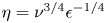 $\eta = \nu ^{3/4} \epsilon ^{-1/4}$, where
 $\nu = \mu /\rho$ is the kinematic viscosity,
 $\rho$ is the fluid mass density and
 $\epsilon$ is the turbulent dissipation rate. This natural mechanism may be imitated for LES theory by conjuring an artificial viscous process to further smooth a frozen snapshot of turbulence, removing small motions below a cutoff length scale,
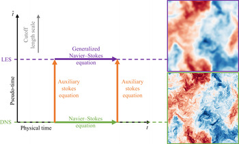
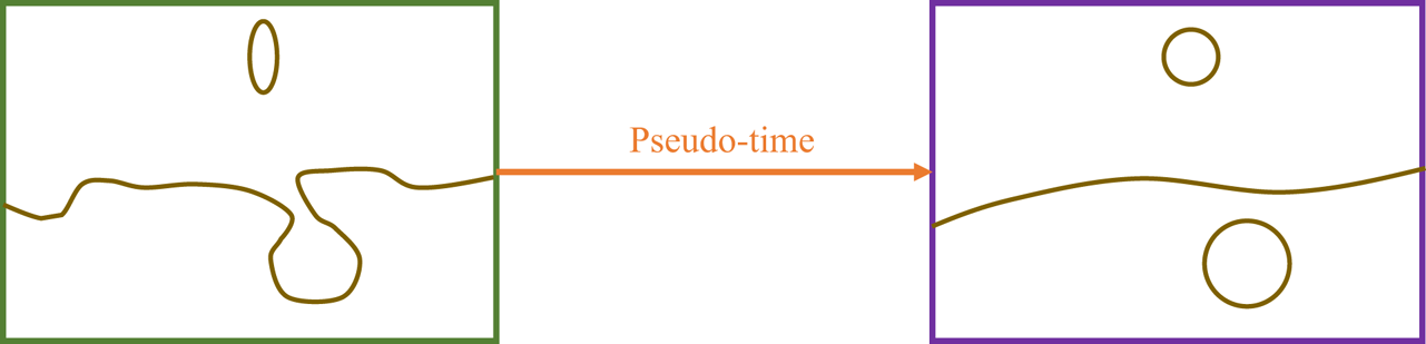
 $\ell > \eta$. The artificial physics-inspired process evolves in a pseudo-time that is independent of physical time. The overall idea of PIC is illustrated in figure 1 and described in detail in the remainder of this section. The final subsection then reviews the spatial filtering theory of LES for comparison and contrast.
PIC for LES defines a generalized velocity field as a function of physical time ( $t$) and pseudo-time (
 $\hat {t} \sim \text {grid-size}^{2}$). The generalized Navier–Stokes equation for the LES velocity in physical time requires a closure model.

2.1. Navier–Stokes equation
For the present purposes, an incompressible flow of a Newtonian fluid is considered. A velocity vector field,  $\boldsymbol {u} = \boldsymbol {u}(\boldsymbol {x},t)$, evolves as a function of space,
 $\boldsymbol {x}$, and time,
 $t$, according to the Navier–Stokes equation
 \begin{equation} \frac{\partial u_i}{\partial t} + \frac{\partial}{\partial x_j}\left[ u_i u_j + p \delta_{ij} - \nu \left( \frac{\partial u_i}{\partial x_j} + \frac{\partial u_j}{\partial x_i} \right) \right] = 0, \quad \frac{\partial u_j}{\partial x_j} = 0.\end{equation}
The pressure (divided by density),  $p(\boldsymbol {x},t)$, enforces the divergence-free condition. A Poisson equation for the pressure follows from the divergence of the Navier–Stokes equation
 \begin{equation} \nabla^{2} p ={-} \frac{\partial u_i}{\partial x_j} \frac{\partial u_j}{\partial x_i}. \end{equation}
Thus, a fully resolved simulation (DNS) evolves (2.1) together with (2.2) in physical time with pseudo-time fixed at zero,  $\hat {t} = 0$, indicated by the green arrow in figure 1.
2.2. Auxiliary Stokes equation
For the physics-inspired approach, a generalized velocity field, 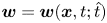 $\boldsymbol {w} = \boldsymbol {w}(\boldsymbol {x}, t; \hat {t})$, is defined as a function of both time,
 $t$, and a pseudo-time,
 $\hat {t}$. The generalized velocity field at
 $\hat {t} = 0$ corresponds to the physical velocity field
 \begin{equation} \boldsymbol{w}(\boldsymbol{x},t; 0) = \boldsymbol{u}(\boldsymbol{x},t).\end{equation}
As  $\hat {t}$ increases, small-scale motions are removed from the generalized velocity field. Thus, the pseudo-time is an indicator of the resolution length scale of the generalized velocity. To accomplish this, an auxiliary Stokes equation may be introduced to govern the pseudo-time evolution
 \begin{equation} \frac{\partial w_i}{\partial \hat{t}} + \frac{\partial}{\partial x_j}\left[ \hat{p}\delta_{ij} - \hat{\nu} \left( \frac{\partial w_i}{\partial x_j} + \frac{\partial w_j}{\partial x_i} \right) \right] = 0, \quad \frac{\partial w_j}{\partial x_j} = 0.\end{equation}
The nonlinear term of the Navier–Stokes equation ( $u_i u_j$) is removed for (2.4), so there is no energy cascade in pseudo-time and hence no resupply of energy to small scales dissipated by pseudo-viscosity,
 $\hat {\nu }(\boldsymbol {x})$. The length scale at which the flow is smoothed may be heuristically estimated as
 $\ell \sim \sqrt {\hat {\nu } \hat {t}}$. A pseudo-pressure,
 $\hat {p}(\boldsymbol {x},t;\hat {t})$, is also introduced to enforce a divergence-free condition for the generalized velocity at all pseudo-times. The divergence of the auxiliary Stokes equation is a Poisson equation for the pseudo-pressure
 \begin{equation} \nabla^{2} \hat{p} = \frac{\partial^{2}}{\partial x_i \partial x_j}\left[ \hat{\nu} \left( \frac{\partial w_i}{\partial x_j} + \frac{\partial w_j}{\partial x_i} \right) \right]. \end{equation}
Thus, a DNS may be artificially coarsened by, instead of applying a spatial filter, advancing (2.4) in pseudo-time together with (2.5) having initial conditions set by (2.3). This is represented in figure 1 by the orange arrows. In the case of a moving reference frame, the coordinate system only advances in physical time. It is frozen in pseudo-time by definition, so that Galilean invariance is satisfied. Note that the pseudo-viscosity is distinct from the idea of an eddy viscosity (or turbulent viscosity) often used to model turbulent flows. The pseudo-viscosity acts only in pseudo-time and simply enables the coarsening procedure that is an alternative to spatial filtering. An eddy viscosity acts in physical time and attempts to approximate the evolution of a coarsened velocity field in physical time, which is considered next.
2.3. Generalized Navier–Stokes equation
Explicit filtering is not typically used in practice for LES. Similarly, it is not envisioned at present that PIC-based LES practice will (necessarily) include the numerical solution of an auxiliary Stokes equation. The significance of (2.4), rather, is its implication for the evolution of the generalized velocity in physical time, keeping  $\hat {t} \sim \ell ^{2}$ fixed based on the grid resolution. This is illustrated by the purple arrow in figure 1 and corresponds to establishing the effective equations for solving a coarsened representation of the flow, which may in practice be done on a coarser grid.
The outcome of the auxiliary Stokes equation ensures that the Navier–Stokes equation must be altered to accurately describe the evolution of the coarsened flow field in physical time. Thus, an effective evolution equation for LES may be derived by finding the appropriate residual force,  $\boldsymbol {F}$, such that
 \begin{equation} \frac{\partial w_i}{\partial t} + \frac{\partial}{\partial x_j}\left[ w_i w_j + \phi\delta_{ij} - \nu \left( \frac{\partial w_i}{\partial x_j} + \frac{\partial w_j}{\partial x_i} \right) \right] = F_i, \quad \frac{\partial w_j}{\partial x_j} = 0. \end{equation}
When  $\hat {t} = 0$, the generalized velocity does satisfy (2.1) because of the initial condition, (2.3). This means that,
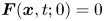 $\boldsymbol {F}(\boldsymbol {x}, t; 0) = 0$.
Because the auxiliary Stokes equation globally conserves momentum in the absence of fluxes through domain boundaries, the residual force must likewise conserve momentum, and it may be written as the divergence of a residual stress tensor
 \begin{equation} F_ i = \frac{\partial \sigma_{ij}}{\partial x_j}. \end{equation}
Thus, the evolution of the generalized velocity in physical time is given by the generalized Navier–Stokes equation
 \begin{equation} \frac{\partial w_i}{\partial t} + \frac{\partial}{\partial x_j}\left[ w_i w_j + \sigma_{ij} + \phi\delta_{ij} - \nu \left( \frac{\partial w_i}{\partial x_j} + \frac{\partial w_j}{\partial x_i} \right) \right] = 0, \quad \frac{\partial w_j}{\partial x_j} = 0.\end{equation}
Note that the divergence-free constraint on the auxiliary Stokes equation implies a divergence-free condition for the physical time evolution as well. This is enforced by a generalized pressure,  $\phi (\boldsymbol {x},t;\hat {t})$, that is distinct from the pseudo-pressure,
 $\hat {p}$, which acts only during pseudo-time evolution. The generalized pressure may be found by solution of the following Poisson equation:
 \begin{equation} \nabla^{2} \phi ={-} \frac{\partial w_i}{\partial x_j} \frac{\partial w_j}{\partial x_i} - \frac{\partial^{2} \sigma_{ij}}{\partial x_i \partial x_j}. \end{equation}
Equation (2.8), together with (2.9) is unclosed in general. The residual stress tensor field must be approximated in terms of the generalized velocity field in order to solve for its evolution. More specifically, only the deviatoric component of  $\boldsymbol {\sigma }$ is material to the closure problem, because any isotropic component may be lumped in with the generalized pressure and found via (2.9). For consistency, it is required that the generalized velocity,
 $\boldsymbol {w}$, evolves according to the Navier–Stokes equation for
 $\hat {t} = 0$. That is, (2.8) must be identical to (2.1) when
 $\hat {t} = 0$. Thus
 \begin{equation} \phi(\boldsymbol{x}, t; 0) = p(\boldsymbol{x},t), \quad \sigma_{ij}(\boldsymbol{x}, t; 0) = 0. \end{equation}
2.4. Residual stress tensor equation
The significance of the above theory is its implications for the mathematical definition of the residual stress tensor, which is found by requiring consistency between the pseudo-time and physical time evolution of the generalized velocity field sketched in figure 1. Specifically,  $\boldsymbol {\sigma }$ may be defined by asserting that advancing the generalized velocity field from
 $(t_0, \hat {t}_0)$ to
 $(t_f, \hat {t}_f)$ must be independent of the path in
 $t$–
 $\hat {t}$ space. Breaking the evolution in
 $t$–
 $\hat {t}$ space into infinitesimal increments, this requirement may be written as
 \begin{equation} \frac{\partial}{\partial \hat{t}}\left( \frac{\partial w_i}{\partial t} \right) =\frac{\partial}{\partial t}\left( \frac{\partial w_i}{\partial \hat{t}} \right),\end{equation}
which is simply the symmetry of mixed partial derivatives. More detailed treatment of the implications of this constraint for the form of the residual stress tensor will be given later.
2.5. Kinetic energy equations
The scale-wise dynamics of kinetic energy is crucial to the representation of turbulent flows. The generalized kinetic energy (per unit mass) in PIC is given by  $\tfrac {1}{2} w_i w_i$. First, consider how kinetic energy evolves in pseudo-time. Multiplying the auxiliary Stokes equation, (2.4), by
 $w_i$ and using a product rule on the viscous term
 \begin{equation} \frac{\partial (\tfrac{1}{2} w_i w_i)}{\partial \hat{t}} + \frac{\partial}{\partial x_j}[ \hat{p} w_j - 2 \hat{\nu} w_i S_{ij} ] ={-} 2 \hat{\nu} S_{ij} S_{ij}, \end{equation}
where  $S_{ij} = \tfrac {1}{2}( \partial w_i/ \partial x_j + \partial w_j/\partial x_i)$ is the generalized strain-rate tensor. As pseudo-time increases, kinetic energy is removed by the pseudo-viscosity at a rate
 $2 \hat {\nu } S_{ij} S_{ij} \geq 0$.
The dynamics of generalized kinetic energy in physical time (at fixed, finite pseudo-time) can be written by multiplying the generalized Navier–Stokes equation, (2.8) by  $w_i$
 \begin{equation} \frac{\partial (\tfrac{1}{2} w_i w_i)}{\partial t} + \frac{\partial}{\partial x_j}\left[ \frac{1}{2} w_i w_i w_j + w_i \sigma_{ij} + \phi w_j - 2 \nu w_i S_{ij} \right] = \sigma_{ij} S_{ij} - 2 \nu S_{ij} S_{ij}. \end{equation}
In addition to direct viscous dissipation,  $2 \nu S_{ij} S_{ij} \geq 0$, the generalized kinetic energy is removed at a rate
 $\varPi = -\sigma _{ij} S_{ij}$. Note that
 $\varPi$ may be positive or negative in general, but that the expectation for turbulence dynamics is a preference toward
 $\varPi > 0$ representing the kinetic energy cascade. That is,
 $\varPi$ represents the rate at which kinetic energy associated with motions larger than
 $\ell \sim \sqrt {\hat {\nu } \hat {t}}$ is passed to motions smaller than
 $\ell$. Thus, an important consideration for any closure model for
 $\sigma _{ij}$ is its ability to remove energy at the proper rate to mimic the energy cascade.
2.6. Juxtaposition with spatial filtering
The traditional approach to LES theory is based on developing equations for the filtered velocity field (Leonard Reference Leonard1975; Germano Reference Germano1992)
 \begin{equation} \bar{u}_i^{\ell}(\boldsymbol{x}, t) = \iiint G^{\ell}(\boldsymbol{r}) u_i(\boldsymbol{x} + \boldsymbol{r}, t) \, {{\rm d}} \boldsymbol{r}, \quad \mathcal{F}\{ \bar{u}_i^{\ell} \} = (2{\rm \pi} )^{3}\mathcal{F}\{ G^{\ell}\} \mathcal{F}\{ u_i \}.\end{equation}
The relative width of the filter is  $\ell$, with larger values of
 $\ell$ resulting in coarser fields. The notation
 $\mathcal {F}$ is used for a Fourier transform in three dimensions. The definition used here for an arbitrary field
 $a$ is
 \begin{equation} \mathcal{F}\{ a \}(\boldsymbol{k}) = \frac{1}{(2{\rm \pi})^{3}} \iiint a(\boldsymbol{x}) \exp( -{\rm i} \boldsymbol{k}\cdot\boldsymbol{x} ) \, {{\rm d}}\kern0.06em \boldsymbol{x}. \end{equation}
The three-dimensional inverse Fourier transform for an arbitrary function  $b$ is therefore
 \begin{equation} \mathcal{F}^{{-}1}\{ b \}(\boldsymbol{x}) = \iiint b(\boldsymbol{k}) \exp( {\rm i} \boldsymbol{k}\cdot\boldsymbol{x} ) \, {{\rm d}} \boldsymbol{k}. \end{equation}
This Fourier transform definition is commonly used for turbulence theory, e.g. (Tennekes & Lumley Reference Tennekes and Lumley1972; Monin & Yaglom Reference Monin and Yaglom1975; Pope Reference Pope2000).
LES practitioners rarely rely on a specific filter kernel shape. Common filter shapes used for theoretical appraisals include top-hat, spectral cutoff and Gaussian kernels (Borue & Orszag Reference Borue and Orszag1998). For example, the Gaussian filter kernel is given by
 \begin{equation} G^{\ell}(\boldsymbol{r}) = \frac{1}{(2{\rm \pi} \ell)^{3/2}} \exp\left( - \frac{|\boldsymbol{r}|^{2}}{2\ell^{2}}\right), \quad (2{\rm \pi})^{3}\mathcal{F}\{G^{\ell}\}(\boldsymbol{k}) = \exp\left( -\frac{1}{2} |\boldsymbol{k}|^{2} \ell^{2} \right). \end{equation}
The Gaussian filter provides a balanced trade-off between localization in physical space and wavenumber space, with exponential-of-square dropoff in both.
For a more general class of filter shapes, the Navier–Stokes equation, (2.1), may be filtered to yield an equation for the filtered velocity field
 \begin{equation} \frac{\partial \bar{u}_i^{\ell}}{\partial t} + \frac{\partial}{\partial x_j}\left[ \bar{u}_i^{\ell} \bar{u}_j^{\ell} + \tau_{ij}^{\ell} + \bar{p}^{\ell}\delta_{ij} - \nu \left( \frac{\partial \bar{u}_i^{\ell}}{\partial x_j} + \frac{\partial \bar{u}_j^{\ell}}{\partial x_i} \right) \right] = \mathcal{C}_i, \quad \frac{\partial \bar{u}_j^{\ell}}{\partial x_j} = \mathcal{D}.\end{equation}
Here, the subfilter stress tensor,  $\tau _{ij}^{\ell } = \overline {u_i u_j}^{\ell } - \bar {u}_i^{\ell } \bar {u}_j^{\ell }$, plays a role analogous to that of the residual stress tensor in PIC,
 $\sigma _{ij}$, although their mathematical definitions may differ. Also, the filtered pressure,
 $\bar {p}^{\ell }$, is analogous to the generalized pressure in PIC,
 $\phi$.
The vector  $\boldsymbol {{\mathcal {C}}}$ and scalar
 $\mathcal {D}$ in (2.18a,b) represent commutator terms that are zero if the filtering operation is spatially uniform, i.e.
 $\ell \neq \ell (\boldsymbol {x})$. In the case of spatially varying filter width, these commutator errors arise and (theoretically) require additional treatment for LES modelling (Ghosal & Moin Reference Ghosal and Moin1995; Langford & Moser Reference Langford and Moser2001; Moser et al. Reference Moser, Haering and Yalla2021; Yalla et al. Reference Yalla, Oliver, Haering, Engquist and Moser2021).
The kinetic energy of the filtered velocity field evolves as
 \begin{equation} \frac{\partial (\tfrac{1}{2} \bar{u}_i^{\ell} \bar{u}_i^{\ell})}{\partial t} + \frac{\partial}{\partial x_j}\left[ \frac{1}{2} \bar{u}_i^{\ell} \bar{u}_i^{\ell} \bar{u}_j^{\ell} + \bar{u}_i \tau_{ij}^{\ell} + \bar{p}^{\ell} \bar{u}_j^{\ell} - 2 \nu \bar{u}_i^{\ell} \bar{s}_{ij}^{\ell} \right] = \tau_{ij}^{\ell} \bar{s}_{ij}^{\ell} - 2 \nu \bar{s}_{ij}^{\ell} \bar{s}_{ij}^{\ell}. \end{equation}
The strain-rate tensor is  $s_{ij} = \tfrac {1}{2}( \partial u_i / \partial x_j + \partial u_j / \partial x_i )$ and the filtered strain-rate tensor is
 $\bar {s}_{ij}^{\ell } = \tfrac {1}{2} ( \partial \bar {u}_i^{\ell } / \partial x_j + \partial \bar {u}_j^{\ell } / \partial x_i )$. The two sinks of the filtered kinetic energy are analogous to those of the generalized kinetic energy in (2.13).
The above derivation presumed an unbounded domain in the filter definition. Section 3 explores the similarity between PIC and filtering in the context of unbounded flows with uniform resolution. Even in this case, PIC provides useful insight. Then, § 4 shows how PIC may be extended to more complex flows, including those which represent a challenge to the spatial filtering approach to LES theory.
3. Unbounded flows with uniform resolution
3.1. Equivalence of PIC with Gaussian filtering
For unbounded flows with uniform resolution (uniform  $\hat {\nu }$), the pseudo-pressure satisfies a Laplace equation in free space, so
 $\hat {p} = 0$. That is, the pseudo-pressure is not needed to enforce the divergence-free condition on the generalized velocity. In this case, the auxiliary Stokes equation simplifies to
 \begin{equation} \frac{\partial w_i}{\partial \hat{t}} = \hat{\nu} \nabla^{2} w_i, \quad w_i(\boldsymbol{x}, t; 0) =u_i(\boldsymbol{x}, t).\end{equation}
The formal solution to (3.1a,b) in an unbounded domain is readily obtained
 \begin{equation} w_i(\boldsymbol{x}, t; \hat{t}) = \iiint \frac{1}{( 4 {\rm \pi}\hat{\nu} \hat{t} )^{3/2}} \exp\left( - \frac{|\boldsymbol{r}|^{2}}{4 \hat{\nu} \hat{t}} \right) u_i(\boldsymbol{x}+\boldsymbol{r}, t) \, {{\rm d}} \boldsymbol{r} \equiv \bar{u}_i^{\ell}(\boldsymbol{x}, t), \end{equation}
which is precisely a Gaussian filter with width  $\ell = \sqrt {2\hat {\nu }\hat {t}}$. Therefore, the PIC approach is precisely equivalent to spatial filtering with a Gaussian kernel for unbounded flows with uniform resolution. All the strengths and theoretical insights of spatial filtering naturally carry over, but a new perspective on the residual stress tensor also emerges.
3.2. PIC expression for the residual stress tensor
With the equivalence to Gaussian filtering established for PIC of unbounded flows with uniform resolution, the mathematical definition of the residual stress tensor could be straightforwardly written as  $\sigma _{ij} = \tau _{ij} \equiv \overline {u_i u_j}^{\ell } - \bar {u}_i^{\ell } \bar {u}_j^{\ell }$. However, insights beyond those arrived at via spatial filtering may be obtained by following the PIC logic further in the form of (2.11).
In the following, flow subjected to an arbitrary (divergence-free) forcing function,  $\boldsymbol {f}(\boldsymbol {x},t)$ is considered, so (2.1) becomes
 \begin{equation} \frac{\partial u_i}{\partial t} + \frac{\partial}{\partial x_j}\left[ u_i u_j + p \delta_{ij} - \nu \left( \frac{\partial u_i}{\partial x_j} + \frac{\partial u_j}{\partial x_i} \right) \right] = f_i, \quad \frac{\partial u_j}{\partial x_j} = 0.\end{equation}
The generalized Navier–Stokes equations are likewise supplemented with a generalized force,  $\boldsymbol {g}(\boldsymbol {x},t)$, that represents the impact of the physical forcing on the coarsened flow representation
 \begin{equation} \frac{\partial w_i}{\partial t} + \frac{\partial}{\partial x_j}\left[ w_i w_j + \sigma_{ij} + \phi\delta_{ij} - \nu \left( \frac{\partial w_i}{\partial x_j} + \frac{\partial w_j}{\partial x_i} \right) \right] = g_i, \quad \frac{\partial w_j}{\partial x_j} = 0.\end{equation}
Substituting equations (3.1a) and (3.4) into (2.11)
 \begin{equation} \frac{\partial}{\partial \hat{t}}\left( \nu \nabla^{2} w_i - \frac{\partial \phi}{\partial x_i} - \frac{\partial w_i w_j}{\partial x_j} - \frac{\partial \sigma_{ij}}{\partial x_j} + g_i \right) - \frac{\partial}{\partial t}( \hat{\nu} \nabla^{2} w_i ) = 0, \end{equation}
and rearranging in terms of time and pseudo-time derivatives,
 \begin{equation} \nu \nabla^{2} \left(\frac{\partial w_i}{\partial \hat{t}}\right) - \frac{\partial}{\partial x_i}\left(\frac{\partial \phi}{\partial \hat{t}}\right) - \frac{\partial}{\partial x_j}\left(w_i \frac{\partial w_j}{\partial \hat{t}} + w_j \frac{\partial w_i}{\partial \hat{t}}\right) - \frac{\partial}{\partial x_j}\left( \frac{\partial \sigma_{ij}}{\partial \hat{t}} \right) + \frac{\partial g_i}{\partial \hat{t}} = \hat{\nu} \nabla^{2} \left(\frac{\partial w_i}{\partial t} \right), \end{equation}
and further substitution of (3.1a) and (3.4)
 \begin{align} &\nu \nabla^{2} (\hat{\nu} \nabla^{2} w_i ) - \frac{\partial}{\partial x_i}\left(\frac{\partial \phi}{\partial \hat{t}}\right) - \frac{\partial}{\partial x_j}(\hat{\nu} w_i \nabla^{2} w_j + \hat{\nu} w_j \nabla^{2} w_i ) - \frac{\partial}{\partial x_j}\left( \frac{\partial \sigma_{ij}}{\partial \hat{t}} \right) + \frac{\partial g_i}{\partial \hat{t}} \nonumber\\ &\quad = \hat{\nu} \nabla^{2} \left( \nu \nabla^{2} w_i - \frac{\partial \phi}{\partial x_i} - \frac{\partial w_i w_j}{\partial x_j} - \frac{\partial \sigma_{ij}}{\partial x_j} + g_i \right). \end{align}
Now, further simplification leads to
 \begin{equation} {-}\frac{\partial}{\partial x_j}\left( \frac{\partial \sigma_{ij}}{\partial \hat{t}} - \hat{\nu} \nabla^{2} \sigma_{ij} - 2 \hat{\nu} \frac{\partial w_i}{\partial x_k} \frac{\partial w_j}{\partial x_k} + \frac{\partial \phi}{\partial \hat{t}} \delta_{ij} - \hat{\nu}\nabla^{2} \phi \delta_{ij} \right) = \frac{\partial g_i}{\partial \hat{t}} - \hat{\nu} \nabla^{2} g_i.\end{equation}
Equation (3.8) simply expresses the condition necessary for (3.4) to correctly describe the large-scale dynamics embodied in the generalized velocity at finite pseudo-time. Because the residual stress should be disentangled from the (arbitrary) forcing function, both sides for (3.8) should be set to zero. Setting the right-hand side to zero, the generalized forcing function may be recognized as the Gaussian-filtered force, cf. (3.1a,b)
 \begin{equation} \frac{\partial g_i}{\partial \hat{t}} = \hat{\nu} \nabla^{2} g_i, \quad g_i(\boldsymbol{x}, t; 0) = f_i(\boldsymbol{x}, t). \end{equation}
The left-hand side of (3.8), once set to zero, may be simplified. Namely, the terms involving the generalized pressure,  $\phi$, may be removed on either of two considerations. First, the generalized pressure may be identified with the Gaussian-filtered pressure
 \begin{equation} \frac{\partial \phi}{\partial \hat{t}} = \hat{\nu} \nabla^{2} \phi, \quad\phi(\boldsymbol{x}, t; 0) = p(\boldsymbol{x}, t). \end{equation}
Alternatively, and more generally, the dynamics of the generalized velocity depends only on the deviatoric part of the residual stress tensor, so any isotropic contribution can be safely ignored.
A sufficient condition for satisfying (3.8) and thus (2.11) is
 \begin{equation} \frac{\partial \sigma_{ij}}{\partial \hat{t}} = \hat{\nu} \nabla^{2} \sigma_{ij} + 2 \hat{\nu} \frac{\partial w_i}{\partial x_k} \frac{\partial w_j}{\partial x_k}. \end{equation}
This is a forced diffusion equation in pseudo-time for  $\boldsymbol {\sigma }$, and its formal solution in unbounded space is also readily obtained
 \begin{align} \sigma_{ij}(\boldsymbol{x}, t; \hat{t}) = \int_{0}^{\hat{t}} \left[ \iiint \frac{1}{( 4 {\rm \pi}\hat{\nu} (\hat{t}-t^{\prime}) )^{3/2}} \exp\left( - \frac{|\boldsymbol{r}|^{2}}{4 \hat{\nu} (\hat{t} - t^{\prime})} \right) \frac{\partial w_i}{\partial x_k} \frac{\partial w_j}{\partial x_k}(\boldsymbol{x}+\boldsymbol{r}, t; t^{\prime}) \, {{\rm d}} \boldsymbol{r} \right] \, {{\rm d}}t^{\prime}. \end{align}
The residual stress at pseudo-time  $\hat {t}$ may thus be interpreted as an integral over all earlier pseudo-times,
 $0 \leq t^{\prime } \leq \hat {t}$, of the velocity gradient product at
 $t^{\prime }$ smoothed by a pseudo-viscosity from its earlier pseudo-time up until the pseudo-time at which the residual stress is evaluated, i.e. over the pseudo-time range
 $\hat {t} - t^{\prime }$.
3.3. Insights into the energy cascade
The equivalence of PIC with Gaussian spatial filtering may be invoked, in the case of unbounded flows with uniform resolution, to rephrase the subfilter stress tensor of filtering theory in terms of multiscale velocity gradients. Dividing equation (3.11) by  $2 \hat {\nu }$, with the established relation
 $\ell ^{2} = 2 \hat {\nu } \hat {t}$
 \begin{equation} \frac{\partial \tau_{ij}}{\partial (\ell^{2})} = \frac{1}{2} \nabla^{2} \tau_{ij} + \frac{\partial \bar{u}_i^{\ell}}{\partial x_k} \frac{\partial \bar{u}_j^{\ell}}{\partial x_k}, \end{equation}
therefore has a formal solution, (3.12), that can itself be written in terms of an integral of Gaussian-filtered velocity gradients at all scales  $0 \leq \sqrt {\alpha } \leq \ell$
 \begin{equation} \tau_{ij} = \int_{0}^{\ell^{2}} \overline{\frac{\partial \bar{u}_i^{\sqrt{\alpha}}}{\partial x_k} \frac{\partial \bar{u}_j^{\sqrt{\alpha}}}{\partial x_k}}^{\beta} \, {{\rm d}} \alpha, \end{equation}
where  $\beta = \sqrt {\ell ^{2} - \alpha }$ is the width of the complementary filter which smooths from scale
 $\sqrt {\alpha }$ to scale
 $\ell$.
Invoking the definition of the generalized second moment from Germano (Reference Germano1992)
 \begin{equation} \tau^{\ell}(a,b) = \overline{a b}^{\ell} - \bar{a}^{\ell} \bar{b}^{\ell}, \end{equation}
of which the subfilter stress tensor is one special case 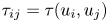 $\tau _{ij} = \tau (u_i, u_j)$, the PIC-based phrasing of the Gaussian filter's stress tensor can be split into resolved-scale and subfilter-scale contributions
 \begin{equation} \tau_{ij} = \ell^{2} \frac{\partial \bar{u}_i^{\ell}}{\partial x_k} \frac{\partial \bar{u}_j^{\ell}}{\partial x_k} + \int_{0}^{\ell^{2}} \tau^{\beta}\left( \frac{\partial \bar{u}_i^{\sqrt{\alpha}}}{\partial x_k}, \frac{\partial \bar{u}_j^{\sqrt{\alpha}}}{\partial x_k} \right)\, {{\rm d}} \alpha. \end{equation}
The first of the two terms on the right-hand side is the nonlinear gradient model, which by itself performs well in a priori testing compared with eddy viscosity models (Clark et al. Reference Clark, Ferziger and Reynolds1979; Borue & Orszag Reference Borue and Orszag1998). The second term shows how such a model leaves out smaller-scale (unresolved) content. Further decomposing the filtered velocity gradients in (3.16) into strain rate and vorticity, and forming the product 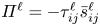 $\varPi ^{\ell } = -\tau _{ij}^{\ell } \bar {s}_{ij}^{\ell }$, the local energy cascade rate may be written in terms of vorticity stretching and strain self-amplification
 \begin{equation} \varPi^{\ell} = \varPi_{s1}^{\ell} + \varPi_{\omega 1}^{\ell} + \varPi_{s2}^{\ell} + \varPi_{\omega 2}^{\ell} + \varPi_{c}^{\ell}, \end{equation}
where
 $$\begin{gather} \varPi_{s1}^{\ell} ={-}\ell^{2} \bar{s}_{ij}^{\ell} \bar{s}_{jk}^{\ell} \bar{s}_{ki}^{\ell} = \text{strain-rate self-amplification at scale } \ell, \end{gather}$$
 $$\begin{gather}\varPi_{\omega 1}^{\ell} = \frac{1}{4} \ell^{2} \bar{s}_{ij}^{\ell} \bar{\omega}_{i}^{\ell} \bar{\omega}_j^{\ell} = \text{vorticity stretching at scale } \ell, \end{gather}$$
 $$\begin{gather}\varPi_{s2}^{\ell} ={-} \bar{s}_{ij}^{\ell} \int_{0}^{\ell^{2}} \tau_{\beta}( \bar{s}_{jk}^{\sqrt{\alpha}}, \bar{s}_{ki}^{\sqrt{\alpha}} ) \, {{\rm d}}\alpha = \text{multiscale strain amplification by strain at } \ell, \end{gather}$$
 $$\begin{gather}\varPi_{\omega 2}^{\ell} = \bar{s}_{ij}^{\ell} \int_{0}^{\ell^{2}} \tau_\beta(\bar{\omega}_i^{\sqrt{\alpha}}, \bar{\omega}_j^{\sqrt{\alpha}}) \, {{\rm d}} \alpha = \text{multiscale vorticity stretching by strain at } \ell, \end{gather}$$
 $$\begin{gather}\varPi_{c}^{\ell} = 2 \bar{s}_{ij}^{\ell} \int_{0}^{\ell^{2}} \tau_\beta( \bar{s}_{jk}^{\sqrt{\alpha}}, \bar{\varOmega}_{ki}^{\sqrt{\alpha}} ) \,{{\rm d}} \alpha= \text{multiscale vortex thinning by strain at } \ell. \end{gather}$$
In this way, the rephrasing of spatial filtering in terms of PIC for unbounded flows with uniform resolution leads to a unique theoretical insight: the exact relation of commonly invoked mechanisms to the energy cascade. For more details, the reader is referred to Johnson (Reference Johnson2020, Reference Johnson2021a). A treatment of the topic for a broader audience is given in Johnson (Reference Johnson2021b).
DNS of homogeneous isotropic turbulence demonstrates that the multiscale gradient terms in  $\boldsymbol {\tau }$ align closely with the filtered strain-rate tensor (Johnson Reference Johnson2021a). The eddy viscosity model is thus a good approximation for the second term on the right-hand side of (3.16). Overall, this suggests the applicability of a mixed model, with
 $\boldsymbol {\sigma } = \boldsymbol {\tau }$ being the sum of nonlinear gradient and eddy viscosity terms (Vreman et al. Reference Vreman, Geurts and Kuerten1994).
3.4. An alternative to the Germano identity
The dynamic procedure (Germano et al. Reference Germano, Piomelli, Moin and Cabot1991) based on the Germano identity (Germano Reference Germano1992) is one of the most common direct uses of spatial filtering theory in LES practice. The basic idea is that coefficients for a given model may be estimated from the resolved scales using a test filter larger than the grid size. A similar procedure may be developed with PIC via the dependence of  $\boldsymbol {\sigma }$ on the cutoff scale (i.e. pseudo-time).
This may be briefly demonstrated for a generic eddy viscosity model
 \begin{equation} \sigma_{ij}^{(d)} \approx{-} 2 \nu_T S_{ij}.\end{equation}
First, (3.23) is substituted into (3.11) and the spatial variability of  $\nu _T$ is neglected (for convenience, as commonly done for the Smagorinsky coefficient)
 \begin{equation} -2 S_{ij} \frac{\partial \nu_T}{\partial \hat{t}} = 2 \hat{\nu} \left( \frac{\partial w_i}{\partial x_k} \frac{\partial w_j}{\partial x_k} - \frac{1}{3} \frac{\partial w_m}{\partial x_n} \frac{\partial w_m}{\partial x_n} \delta_{ij} \right). \end{equation}
The above expression may be modified to the Smagorinsky form and the spatial variability of the filtered strain rate may also be factored in, if desired.
Second, Kolmogorov (Reference Kolmogorov1941) scaling is assumed,  $\nu _T \sim \ell ^{4/3} \sim \hat {t}^{2/3}$, so that the variation of the eddy viscosity in pseudo-time may be evaluated,
 ${\partial \nu _T}/{\partial \hat {t}} = \frac {2}{3} ({\nu _T}/{\hat {t}})$. Then (3.26) becomes
 \begin{equation} -\frac{4}{3} S_{ij} \nu_T = \ell^{2} \left( \frac{\partial w_i}{\partial x_k} \frac{\partial w_j}{\partial x_k} - \frac{1}{3} \frac{\partial w_m}{\partial x_n} \frac{\partial w_m}{\partial x_n} \delta_{ij} \right), \end{equation}
where  $\ell ^{2} = 2 \hat {\nu } \hat {t}$. This equation is over-determined because, in general, a scalar
 $\nu _T$ will not be found that can satisfy the full tensor equation. Therefore, as is typical for dynamic procedures, a least-squares procedure is employed (Lilly Reference Lilly1992). This step leads to a projection on
 $S_{ij}$ that carries the physical meaning of matching the energy cascade rate. The resulting expression for the eddy viscosity is
 \begin{equation} \nu_T = \frac{3 \ell^{2}}{4} \frac{A_{ik} A_{jk} A_{ij}}{S_{mn} S_{mn}} = \frac{3\ell^{2}}{4} \frac{\frac{1}{4} W_i S_{ij} W_j - S_{ij} S_{jk} S_{ki}}{S_{mn} S_{mn}},\end{equation}
where  $A_{ij} = \partial w_i / \partial x_j$ is the generalized velocity gradient tensor,
 $S_{ij} = \tfrac {1}{2} (A_{ij} + A_{ji})$ is the generalized strain-rate tensor and
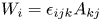 $W_{i} = \epsilon _{ijk} A_{kj}$ is the generalized vorticity. The denominator of this relation is positive–definite. The numerator represents the sum of vortex stretching and strain-rate self-amplification, which is positive on average for turbulent flows. Local negative values of the numerator may necessitate averaging or clipping strategies as done in the Germano-based dynamic procedure.
Johnson (Reference Johnson2021a) demonstrated that the eddy viscosity approximation is more physically accurate for the only part of the residual stress tensor
 \begin{equation} e_{ij} = \sigma_{ij} - 2 \hat{\nu} \hat{t} \frac{\partial w_i}{\partial x_k} \frac{\partial w_j}{\partial x_k}, \end{equation}
which represents multiscale vortex stretching and strain-rate amplification in (3.16). It may be shown from (3.1a,b) and (3.11) that
 \begin{equation} \frac{\partial e_{ij}}{\partial \hat{t}} = \hat{\nu} \nabla^{2} e_{ij} + 4 \hat{\nu}^{2} \hat{t} \frac{\partial^{2} w_i}{\partial x_m \partial x_n} \frac{\partial^{2} w_j}{\partial x_m \partial x_n}. \end{equation}
Substituting the eddy viscosity approximation, (3.23), for  $e_{ij}^{(d)}$ rather than the full residual stress tensor,
 $\sigma _{ij}^{(d)}$, and again assuming
 $\nu _T \sim \hat {t}^{2/3}$ with a least-squares approach leads to a ‘dynamic’ mixed model
 \begin{equation} \sigma_{ij}^{(d)} = \ell^{2} (A_{ik} A_{jk})^{(d)} - 2 \nu_T S_{ij}, \quad \nu_T ={-} \frac{3 \ell^{4}}{4} \frac{B_{ikl} S_{ij} B_{jkl}}{S_{mn} S_{mn}}, \end{equation}
where  $B_{ijk} = \partial ^{2} w_i / \partial x_j \partial x_k$ and
 $\ell ^{2} = 2 \hat {\nu }\hat {t}$. The appearance of the second derivative of the generalized velocity field in the mixed model is less practical when numerical errors are inherent in assessing spatial derivatives. Nonetheless, (3.29a,b) provides a useful initial test for assessing the relative strengths of PIC theory.
3.5. A priori testing
DNS of homogeneous isotropic turbulence is used for a priori tests reported in this subsection. The incompressible Navier–Stokes equation, (2.1), is solved using a pseudo-spectral method with  $1024$ collocation points in each direction. The fully resolved velocity field,
 $\boldsymbol {u}$, is advanced in time with a second-order Adams–Bashforth scheme, and the pressure
 $p$ simply enforces the divergence-free condition. The
 $2\sqrt {2}/3$ rule for wavenumber truncation is used with phase-shift dealiasing (Patterson & Orszag Reference Patterson and Orszag1971). The forcing,
 $\boldsymbol {f}$, is specifically designed to maintain constant kinetic energy in the first two wavenumber shells.
The simulation was initialized using a Gaussian random velocity field satisfying a model turbulent energy spectrum (Pope Reference Pope2000). The simulation was first run through a startup period to reach statistical stationarity. Then, statistics are computed over six large-eddy turnover times. The Taylor-scale Reynolds number is approximately  $Re_\lambda = 400$ with grid resolution
 $k_{max} \eta = 1.4$. The integral length scale is approximately
 $20\,\%$ of the periodic box size of
 $2{\rm \pi}$ and
 $L/\eta = 460$. The skewness of the longitudinal velocity gradient is
 $-0.58$, and the flatness of the longitudinal and transverse velocity gradients are
 $8.0$ and
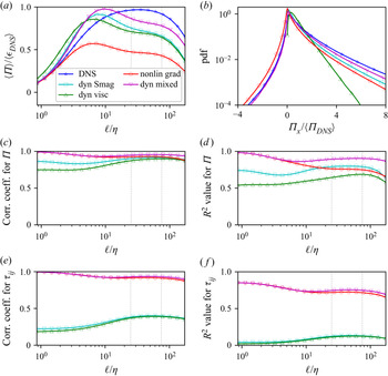
 $12.4$, respectively, in reasonable agreement with previous simulations (Ishihara et al. Reference Ishihara, Kaneda, Yokokawa, Itakura and Uno2007). The a priori assessment is carried out for the ‘dynamic’ viscosity model, (3.26), and ‘dynamic’ mixed model, (3.29a,b), along with existing popular models including the standard dynamic Smagorinsky model (Germano et al. Reference Germano, Piomelli, Moin and Cabot1991; Lilly Reference Lilly1992) and nonlinear gradient model (Clark et al. Reference Clark, Ferziger and Reynolds1979; Borue & Orszag Reference Borue and Orszag1998). For all three dynamic models, spatial averaging is used for the numerator and denominator of the Smagorinsky coefficient or eddy viscosity. The results are shown in figure 2. For this case, PIC and Gaussian filtering are equivalent so the language of each approach is used interchangeably.
A priori comparison of new dynamic eddy viscosity (‘dyn visc’) and dynamic mixed (‘dyn mixed’) models with DNS results and existing models: dynamic Smagorinsky (‘dyn Smag’) and nonlinear gradient model (‘nonlin grad’): (a) mean cascade rate, (b) probability density function of energy cascade rate at  $\ell = 46 \eta$, (c,d) correlation coefficient and R
 $^{2}$ coefficient (also known as the coefficient of determination) for the energy cascade rate, respectively, (e,f) correlation coefficient and R
 $^{2}$ coefficient for the full residual stress tensor, respectively. Two vertical dashed grey lines indicate rough bounds for the approximate inertial subrange of scales in the DNS,
 $25 \leq \ell /\eta \leq 75$.

Perhaps the most important practical consideration for LES models is providing the proper rate of energy removal to unresolved scales. Figure 2(a) shows the average cascade rate,  $\varPi$, as a function of filter width,
 $\ell = \sqrt {2 \hat {\nu } \hat {t}}$, normalized by the average dissipation rate in the unfiltered DNS. The blue curve with star symbols shows that the cascade rate is nearly equal to the dissipation rate for
 $25 \lesssim \ell / \eta \lesssim 75$, an approximate inertial range for the simulation. The cascade rate decays to zero as
 $\ell$ decreases because viscous dissipation becomes significant near the Kolmogorov scale. The other four curves indicate the extent to which the four models reproduce the correct cascade rate when applied directly to coarsened DNS data. As is well known, the nonlinear gradient model is under-dissipative, especially in the inertial range, and the dynamic Smagorinsky model provides a better approximation of the energy removal rate. The PIC-based dynamic eddy viscosity model performs very similarly to the filter-based dynamic Smagorinsky model. The PIC-based dynamic mixed model is confirmed to remove energy at a higher rate in the inertial range than the nonlinear gradient or eddy viscosity models on their own.
The probability density function (PDF) of the energy cascade rate,  $\varPi$, for each model at
 $\ell = 46 \eta$ is shown in figure 2(b) along with the coarsened DNS result. The DNS data indicate the existence of some backscatter, but the distribution is strongly skewed toward positive cascade rates. The two eddy viscosity models do not allow any backscatter by construction due to the spatial averaging used as part of the dynamic procedure. The nonlinear gradient and PIC-based dynamic mixed model provide relatively appropriate probabilities of backscatter, with the mixed model having the best overall agreement with DNS.
Figures 2(c) and 2(d) show the correlation coefficient and R-squared value based on each model's point-by-point prediction of the cascade rate,  $\varPi$. An R-squared value of one indicates a perfect model. All four models are highly correlated with DNS in the inertial range, but the absolute error measured by the R-squared value shows more variation in the models performances. Both metrics show that the PIC-based dynamic mixed model is in closest agreement with DNS. Figures 2(e) and 2(f) show the correlation coefficients and R-squared values based on the full residual (subfilter) stress tensor. The stress tensor is known to align poorly with the strain-rate tensor, so the eddy viscosity models perform poorly for both metrics. The nonlinear gradient model performs quite well and the dynamic mixed model shows only slight improvement. The major benefit of the mixed model over the nonlinear gradient model has already been demonstrated in figure 2(a).
3.6. A posteriori testing
LESs were performed using three stress models: Smagorinsky, PIC-based dynamic eddy viscosity (3.26), and PIC-based dynamic mixed (3.29a,b). The same pseudo-spectral code from the DNS is used. The Smagorinsky coefficient is not determined dynamically for the LES, but was manually chosen to produce accurate results. For the two PIC-based dynamic models, spatial averaging is used for the numerator and denominator of the eddy viscosity, so that the eddy viscosity does not vary in space for either. As such, the simulation with the PIC-based dynamic eddy viscosity model is essentially a DNS at a lower Reynolds number, with the PIC-based theory setting the viscosity so as to match Gaussian-filtered DNS (fDNS) with a given filter width.
The filter width (pseudo-time) is chosen to be  $\ell / \eta = 24$, which is at the small-scale end of the inertial range identified in the a priori tests. The following grid resolutions were tested:
 $64^{3}$,
 $128^{3}$ and
 $256^{3}$. These correspond to
 $k_{{max}} \ell = 1.5$,
 $3.0$ and
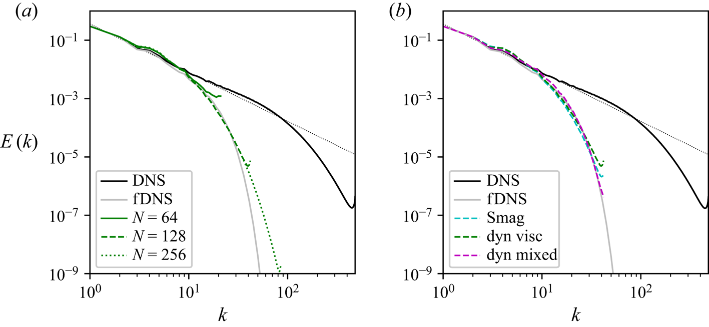
 $6.0$. The DNS results are filtered with a Gaussian kernel (equivalent to PIC) for direct comparison with the LES results from each model. Figure 3(a) shows the energy spectra from LES simulations at each of the three resolutions with the PIC-based dynamic eddy viscosity model. The spectra from each resolution overlap until wavenumbers close to
 $k_{{max}}$, where a slight pileup occurs. The results from
 $128^{3}$ and
 $256^{3}$ are very similar, indicating grid convergence, but
 $64^{3}$ is not grid converged. The spectra from the three models are compared at
 $128^{3}$ resolution in figure 3(b). The Smagorinsky model is known to produce a spectrum close to that of a Gaussian filter (Pope Reference Pope2000), as affirmed by the results here. The PIC-based dynamic mixed model produces a spectrum almost indistinguishable from the Gaussian-filtered DNS for the simulation shown here. All three models produce spectra in reasonable agreement. The PIC-based dynamic procedure for determining the eddy viscosity is thus shown to work well for both the pure eddy viscosity and mixed models.
Energy spectra for a posteriori testing: (a) using PIC-based dynamic eddy viscosity model with  $\ell / \eta = 24$ at three different resolutions, and (b) using three different models with
 $k_{{max}} \ell = 3$. A Kolmogorov spectrum,
 $E(k) =1.6 \epsilon ^{2/3} k^{-5/3}$ is shown for reference in both panels.

In addition to testing the energy spectra produced by various LES models, it is also useful to compare local flow topology statistics. Given the importance of strain self-amplification and vorticity stretching to turbulence dynamics, the LES models are compared with filtered DNS in terms of the following two quantities:
 \begin{equation} s^{*} = \frac{-\sqrt{6} S_{ij} S_{jk} S_{ki}}{(S_{mn} S_{mn})^{3/2}} \quad \omega^{*} = \frac{\sqrt{6} W_i S_{ij} W_j}{2 W_k W_k ( S_{mn} S_{mn} )^{1/2}}. \end{equation}
The first,  $s^{*}$, was introduced by Lund & Rogers (Reference Lund and Rogers1994) and quantifies the efficiency of the strain self-amplification contribution to the energy cascade,
 $-1 \leq s^{*} = \varPi _{s1} / \varPi _{s1,{max}} \leq 1$. The second term likewise indicates the efficiency of the vorticity stretching contribution to the cascade,
 $-1 \leq \omega ^{*} = \varPi _{\omega 1} / \varPi _{\omega 1,{max}} \leq 1$. The concept of cascade efficiency was introduced by Ballouz & Ouellette (Reference Ballouz and Ouellette2018) and extended to include the above definitions in Johnson (Reference Johnson2021a). These two quantities describe flow topology in a way most relevant to turbulent cascade physics.
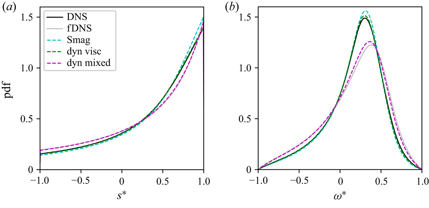
Figure 4 compares the PDFs of  $s^{*}$ and
 $\omega ^{*}$ from LES models and filtered DNS. Results from unfiltered DNS are also shown to highlight the similarity of the eddy viscosity models, particularly the PIC-based dynamic viscosity model, with (unfiltered) DNS. The reason for this is that the eddy viscosity models behave like DNS at lower Reynolds numbers, and thus produce topology statistics similar to the Kolmogorov scales in DNS. However, the results in figure 4 demonstrate that the PIC-based mixed model captures subtle physical differences between viscous-scale and inertial range flow topology statistics.
PDFs of  $s^{*}$ and
 $\omega ^{*}$, (3.30a,b), for LES with three different models compared with DNS and filtered DNS.

Many other metrics can be used to judge the a posteriori accuracy of LES models. It is not the goal at present to thoroughly explore all possibilities. However, a number of highly relevant statistics are summarized in table 1. It may be noted that the PIC-based dynamic mixed model slightly over-predicts the magnitude of velocity gradients, which may also be noticed in the spectra shown in figure 3(b), where a slight over-prediction is noticeable for a range of wavenumbers slightly smaller than the inverse of the filter scale. There appears to be a slight (unphysical) build up of energy not entirely unlike the bottleneck effect commonly observed in DNS and experimental data near the Kolmogorov scale (Falkovich Reference Falkovich1994; Donzis & Sreenivasan Reference Donzis and Sreenivasan2010).
Statistical results from LES and filtered DNS at  $\ell / \eta = 24$ with
 $128^{3}$ resolution (
 $k_{{max}} \ell = 3$). These values were converged when compared with
 $256^{3}$ resolution.

All three models over-predict the fraction of the cascade rate due to single-scale strain self-amplification and vorticity stretching. For the mixed model, this shows that too much energy removal is done through the nonlinear gradient term, and not enough through the eddy viscosity. The longitudinal and transverse velocity gradient skewness and flatness values from the mixed model LES are in fairly good agreement with the filtered DNS. Notice that the dynamic eddy viscosity model leads to too much intermittency (higher skewness and flatness), because it has a spatially uniform eddy viscosity, whereas the local adjustments due to Smagorinsky's eddy viscosity bring intermittency metrics more in line with filtered DNS.
Overall, all three models perform reasonably well in a posteriori tests. Furthermore, the relative advantages of the mixed model are clear, and the success of the PIC-based dynamic scheme is demonstrated. It should be appreciated that PIC theory for LES can facilitate model development well beyond the specific models tested here. The success of these models, however, does motivate future work to develop refined PIC-based models.
4. Toward PIC for more complex flows
In § 3, it was shown that PIC is mathematically equivalent to spatial filtering with a Gaussian kernel for unbounded flows with uniform, isotropic resolution. Even so, the PIC-based approach to LES provided theoretical and modelling insights, including a PIC-based alternative to the Germano-based dynamic procedure that does not require test filtering. Preliminary models showed promising a priori and a posteriori results, but there is more room for future work developing and testing models even for that simple case.
In this section, the extension of PIC to a number of more complex flow scenarios is outlined. The focus is on how the basic theory of PIC provides the flexibility and systematic approach to incorporate features needed for practical application of LES to complex flows.
4.1. Anisotropic resolution
The first step toward LES of more complex flows is a consistent treatment of grid anisotropy. Anisotropic grid resolutions are often unavoidable in simulations with complex geometries. Various treatments of grid anisotropy exist for spatial filtering theory (Bardina et al. Reference Bardina, Ferziger and Reynolds1980; Scotti, Meneveau & Lilly Reference Scotti, Meneveau and Lilly1993; Vreman Reference Vreman2004; Rozema et al. Reference Rozema, Bae, Moin and Verstappen2015; Haering, Lee & Moser Reference Haering, Lee and Moser2019). In practice, simple treatments of grid anisotropy are common, such as using a scalar measure for effective resolution based on a suitable average of resolution in three different directions on an orthogonal grid:  $\varDelta _1$,
 $\varDelta _2$ and
 $\varDelta _3$. Deardorff (Reference Deardorff1970) suggested the use of
 $\varDelta = \sqrt [3]{\varDelta _1 \varDelta _2 \varDelta _3}$ based on the cell volume and Bardina et al. (Reference Bardina, Ferziger and Reynolds1980) used
 $\varDelta = \sqrt {(\varDelta _1^{2} + \varDelta _2^{2} + \varDelta _3^{2})/3}$.
For viscosity-based smoothing, anisotropic resolution is easily introduced using a tensorial pseudo-viscosity aligned with the principal directions of the grid. Thus, (3.1a) for unbounded flows may be modified to incorporate anisotropic resolution effects
 \begin{equation} \frac{\partial w_i}{\partial \hat{t}} = \hat{\nu}_{jk} \frac{\partial^{2} w_i}{\partial x_j \partial x_k}, \quad \frac{\partial w_j}{\partial x_j} = 0.\end{equation}
For uniform resolution, the pseudo-pressure will satisfy the Laplace equation and hence be  $\hat {p} = 0$ in the absence of flow boundaries. In that case, the result will be anisotropic Gaussian filtering aligned with the grid
 \begin{equation} w_i(\boldsymbol{x}, t; \hat{t}) = \iiint \frac{1}{\sqrt{ (2 {\rm \pi})^{3} \det \boldsymbol{C} } } \exp\left( - \frac{1}{2} r_j C_{jk}^{{-}1} r_k \right) u_i(\boldsymbol{x}+\boldsymbol{r}, t) \, {{\rm d}} \boldsymbol{r}. \end{equation}
Here, the covariance tensor,  $C_{ij} = 2 \hat {\nu }_{ij} \hat {t}$, is equivalent to the moment of inertial tensor of Bardina et al. (Reference Bardina, Ferziger and Reynolds1980). The isotropic form, (3.1a,b), is recovered when
 $\hat {\nu }_{ij} = \hat {\nu } \delta _{ij}$. The eigenvalues of
 $\boldsymbol {C}$,
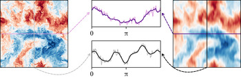
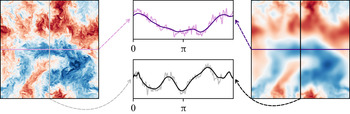
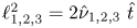 $\ell _{1,2,3}^{2} = 2 \hat {\nu }_{1,2,3} ~\hat {t}$, represent the (square of the) resolution in three directions given by their respective eigenvectors (e.g. the local coordinate frame of an orthogonal grid). The result of anisotropic PIC (i.e. anisotropic Gaussian filtering) is illustrated in figure 5. In this case, the coarsening procedure generates anisotropy in the generalized velocity field from an initially isotropic fully resolved velocity field (Haering et al. Reference Haering, Lee and Moser2019).
A coarsened velocity field using anisotropic pseudo-viscosity on DNS data of homogeneous isotropic turbulence. The resolution length scale ( $\sqrt {2\hat {\nu }\hat {t}}$) in the
 $x$ direction (purple/magenta lines) is one-fourth of that in the
 $y$ direction (black/grey lines).

Substituting equations (2.8) and (4.1a,b) in (2.11), one obtains
 \begin{equation} \frac{\partial \sigma_{ij}}{\partial \hat{t}} = \hat{\nu}_{mn} \frac{\partial^{2} \sigma_{ij}}{\partial x_m \partial x_n} + \hat{\nu}_{mn} \left( \frac{\partial w_i}{\partial x_m} \frac{\partial w_j}{\partial x_n} + \frac{\partial w_i}{\partial x_n} \frac{\partial w_j}{\partial x_m} \right). \end{equation}
The details of the derivation leading to (4.3) follow the same steps as those shown in § 3 leading to (3.11). Indeed, it is readily verified that (3.11) is recovered in the isotropic limit,  $\hat {\nu }_{ij} = \hat {\nu } \delta _{ij}$. The PIC-based dynamic procedure for anisotropic grids can be based on (4.3), which could lead to eddy viscosity models that share some similarities with the anisotropic minimum dissipation model (Rozema et al. Reference Rozema, Bae, Moin and Verstappen2015) and the M43 model (Haering et al. Reference Haering, Lee and Moser2019), while a PIC-based dynamic mixed model may share similarities with that of Vreman (Reference Vreman2004).
4.2. Non-uniform resolution
Uniform grid resolution is useful for some simple canonical turbulent flows, but it is not practical for many naturally occurring and engineered flows. As discussed in the introduction, a non-uniform filter does not commute with spatial differentiation, giving rise to additional terms in the governing equations for filtered fields (Ghosal & Moin Reference Ghosal and Moin1995; Yalla et al. Reference Yalla, Oliver, Haering, Engquist and Moser2021). Most notably, the filtered velocity field is no longer divergence free (Langford & Moser Reference Langford and Moser2001).
In contrast, the PIC approach to the LES equations explicitly enforces a divergence-free condition on the generalized velocity field,  $\boldsymbol {w}$, using a pseudo-pressure,
 $\hat {p}$, in the auxiliary evolution equation in pseudo-time,
 $\hat {t}$. The above theory for uniform resolution was able to ignore the proposed pseudo-pressure due to the form of its Poisson equation, (2.5), which may be alternatively written in terms of pseudo-viscosity gradients
 \begin{equation} \nabla^{2} \hat{p} = 2 \frac{\partial \hat{\nu}}{\partial x_i} \nabla^{2} w_i + \frac{\partial^{2} \hat{\nu}}{\partial x_i \partial x_j}\left( \frac{\partial w_i}{\partial x_j} + \frac{\partial w_j}{\partial x_i} \right), \end{equation}
which reduces to a Laplace equation for uniform pseudo-viscosity (i.e. uniform grid resolution). Non-uniform resolution is represented as spatial variation of the pseudo-viscosity,  $\hat {\nu } = \hat {\nu }(\boldsymbol {x})$, which activates a non-zero pseudo-pressure to enforce the divergence-free condition. Note that, with the non-zero pseudo-pressure, the PIC equations for pseudo-time evolution are no longer purely parabolic, but include an elliptic nature as well. However, the square-of-exponential falloff of the spectral content is still roughly preserved, so that the removal of small scales is still rather efficient compared with other elliptic partial differential equations (Germano Reference Germano1986a,Reference Germanob; Bull & Jameson Reference Bull and Jameson2016).
Figure 6 demonstrates the outcome of PIC with a spatially varying pseudo-viscosity for a velocity field snapshot from DNS of homogeneous isotropic turbulence with  $\hat {\nu }(y) = \hat {\nu }_{max} - (\hat {\nu }_{max} - \hat {\nu }_{min}) \cos (y)$, where
 $0 \leq y \leq 2{\rm \pi}$ is the vertical axis as printed on the page. The rightmost image is of a divergence-free velocity field with variable resolution. The effective resolution is isotropic, but varies in space, with high resolution near the top and bottom (
 $\hat {\nu } \approx \hat {\nu }_{min}$) and low resolution near the centre (
 $\hat {\nu } \approx \hat {\nu }_{max}$).
A (divergence-free) coarsened velocity field using sinusoidally varying pseudo-viscosity applied to DNS data of homogeneous isotropic turbulence. The resolution length scale,  $\sqrt {2\hat {\nu }\hat {t}}$ varies by a factor of
 $4$ between
 $y = 0$ and
 $y = {\rm \pi}$.

The case of non-uniform (isotropic) resolution is useful for reflecting on the PIC approach in general. The goal of PIC is to create LES equations with well-defined closure terms that facilitate effective modelling in ways that improve upon spatial filtering. It is not a central goal of PIC to remain particularly faithful to physical processes during its pseudo-time evolution. The physical processes inspiring the pseudo-time dynamics are useful insomuch as they create helpful representations for LES. This allows some freedom when designing the details of PIC, for example, one may choose to simplify the auxiliary Stokes equation, (2.4), to
 \begin{equation} \frac{\partial w_i}{\partial \hat{t}} ={-}\frac{\partial \hat{p}}{\partial x_i} + \frac{\partial}{\partial x_j}\left[ \hat{\nu} \frac{\partial w_i}{\partial x_j} \right], \quad \frac{\partial w_j}{\partial x_j} = 0, \quad \nabla^{2} \hat{p} = \frac{\partial}{\partial x_j}\left( \frac{\partial \hat{\nu}}{\partial x_i} \frac{\partial w_i}{\partial x_j} \right).\end{equation}
The difference between (2.4) and (4.5a,b) is only material for non-uniform pseudo-viscosity. Either may be used for PIC, and it is not immediately evident which will be most beneficial for LES. More research is needed to elucidate the relative strengths of either.
Substituting equations (4.5a,b) and (2.8) into (2.11) and performing simplifications like those in § 3, one may arrive at the auxiliary equation for the residual stress for general  $\hat {\nu } = \hat {\nu }(\boldsymbol {x})$
 \begin{align} \frac{\partial \sigma_{ij}}{\partial \hat{t}} &= \frac{\partial}{\partial x_k}\left( \hat{\nu} \frac{\partial \sigma_{ij}}{\partial x_k} \right) + 2 \hat{\nu} \frac{\partial w_i }{\partial x_k} \frac{\partial w_j}{\partial x_k} \nonumber\\ &\quad - \left( w_i \frac{\partial w_k}{\partial x_j} + w_j \frac{\partial w_k}{\partial x_i} + \frac{\partial w_i w_k}{\partial x_j} + \frac{\partial \sigma_{ik}}{\partial x_j} - \frac{\partial \hat{p}}{\partial x_j} \delta_{ik} \right) \frac{\partial \hat{\nu}}{\partial x_k} + ( w_i \delta_{jk} + w_j \delta_{ik} ) \frac{\partial \hat{p}}{\partial x_k}. \end{align}
Deviations from (3.11) are proportional to the pseudo-viscosity gradient, as well as the pseudo-pressure. One way to view the extra terms in (4.6) is to view them as consequences of the lack a commutativity between multiplication by  $\hat {\nu }$ and differentiation. The advantage of this PIC formulation is that these commutator terms are built into the residual stress, and so provide a path for extending the use of dynamic procedures and other approaches from uniform resolution to more general cases. Beyond traditional (theory-based) modelling approaches, data-driven techniques may stand to benefit even more from PIC and (4.6). While isotropic non-uniform resolution has been considered here, the same procedure may be used to combine anisotropic and non-uniform grid effects into a single formulation.
4.3. Heat and mass transfer
In addition to complexities introduced by numerical grid effects, PIC provides a holistic approach for reducing the computational DoFs needed to represent turbulence in regimes with additional physical effects beyond unbounded single-phase incompressible flows. The next few subsections touch briefly on a few examples, the simplest of which is passive scalar transport.
For flows with heat or mass transfer described by an advection diffusion equation
 \begin{equation} \frac{\partial T}{\partial t} + u_j \frac{\partial T}{\partial x_j} = \alpha \nabla^{2} T, \end{equation}
the relevant scalar field  $T$ (e.g. temperature or concentration) may be coarsened in a physics-inspired manner using an pseudo-conductivity or pseudo-diffusivity,
 $\hat {\alpha }$, to form a generalized temperature/concentration,
 $\theta$, with pseudo-time evolution given by an auxiliary heat equation
 \begin{equation} \frac{\partial \theta}{\partial \hat{t}} = \hat{\alpha} \nabla^{2} \theta, \quad \frac{\partial \theta}{\partial t} + w_j \frac{\partial\theta}{\partial x_j} = \alpha \nabla^{2} \theta - \frac{\partial q_j}{\partial x_j}, \end{equation}
so that the physical time evolution of the generalized temperature/concentration must include a residual heat/mass flux  $\boldsymbol {q}$. The equality of mixed partial derivatives for
 $\theta$
 \begin{equation} \frac{\partial}{\partial \hat{t}}\left( \frac{\partial \theta}{\partial t} \right) = \frac{\partial}{\partial t}\left( \frac{\partial \theta}{\partial \hat{t}} \right), \end{equation}
may be satisfied by a forced diffusion equation for the residual heat/mass flux
 \begin{equation} \frac{\partial q_i}{\partial \hat{t}} = \hat{\alpha} \nabla^{2} q_i + 2 \hat{\alpha} \frac{\partial w_i}{\partial x_j} \frac{\partial \theta}{\partial x_j}.\end{equation}
Here,  $\hat {\alpha } = \hat {\nu }$ is chosen (unity pseudo-Prandtl number) for convenience. Other choices of pseudo-Prandtl number are possible, but unlikely to be advantageous.
Similar extensions to non-uniform or anisotropic resolution may be found for heat/mass transfer as shown for the momentum equation above. Equation (4.10) can also provide insight into the scale-wise scalar fluctuation dynamics. A turbulent cascade of scalar variance may be linked to the multiscale squeezing of scalar filaments using the formal solution in wall-free flows following the procedure outline for the kinetic energy cascade in § 3. Furthermore, (4.10) can serve as the basis for a PIC-based dynamic procedure for an eddy diffusivity or mixed model for  $\boldsymbol {q}$.
4.4. Wall-bounded turbulent flows
Turbulence near solid boundaries is very common in flows of interest for LES. This is the source of some inconvenience for spatial filtering theory. A uniform filter integral will require flow information outside the fluid domain (Drivas & Nguyen Reference Drivas and Nguyen2018; Kumar et al. Reference Kumar, Quan and Eyink2021). This may be avoided through the use of a filter width which vanishes at the boundary is approached (Bose & Moin Reference Bose and Moin2014), giving rise to commutation errors discussed in § 4.2.
In contrast to spatial filtering, the physics-inspired approach naturally extends to wall-bounded flows. To accomplish this, the auxiliary Stokes equation, (2.4) must be given boundary conditions for  $\boldsymbol {w}$. For example, the use of user-defined boundary conditions for coarsening procedures has been preliminarily investigated (Bae & Lozano-Duran Reference Bae and Lozano-Duran2017, Reference Bae and Lozano-Duran2018). A number of choices are possible depending on the level of near-wall resolution. If the wall-normal grid spacing resolves the viscous sublayer,
 $\ell _y^{+} \sim 1$, then the best choice of boundary conditions is likely Dirichlet,
 $\boldsymbol {w}|_{{wall}} = 0$. Depending on the wall parallel resolution, this approach could facilitate wall-resolved LES (
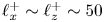 $\ell _x^{+} \sim \ell _z^{+} \sim 50$) or near-wall RANS for hybrid RANS–LES (coarser
 $x$–
 $z$ resolution).
Alternatively, a coarser wall-normal resolution,  $\ell _y \gg 1$, would facilitate development of approximate closures for wall-modelled LES. In this case, Dirichlet boundary conditions could still be used (Bae & Lozano-Duran Reference Bae and Lozano-Duran2021), but other choices such as Robin (Bose & Moin Reference Bose and Moin2014) or Neumann boundary conditions could be used. The choice of boundary conditions for the pseudo-time dynamics would directly set the boundary conditions to be used in LES on the generalized velocity field. Furthermore, complementary boundary conditions on the residual stress tensor,
 $\boldsymbol {\sigma }$, would also need to be specified in such a way as to preserve the integral of momentum transport across the boundary during the pseudo-time evolution so as to facilitate accurate calculations of forces in the LES. For example, in a wall-resolved LES regime, Dirichlet boundary conditions would likely be the best choice for the residual stress in conjunction with Dirichlet velocity boundary conditions. Further research is needed to determine the best approach for wall-modelled LES.
Data-driven techniques may be useful for testing the potential fruitfulness of various choices for the boundary conditions. For example, the art of constructing data-driven wall models may benefit substantially from the PIC-based approach to the LES equations. Sufficiently far from the wall,  $y \gg \ell$, the PIC naturally recovers Gaussian filtering, but near the wall, the PIC theory outlined in this paper provides a method for determining how the choice of boundary conditions influences the residual stress tensor.
4.5. Particle-laden flows
Turbulent flows with small particles also represent a challenge to spatial filtering theory. Lagrangian particle tracking methods, in combination with an Eulerian representation of the carrier fluid, are increasingly common to computing particle-laden flows. In the PIC approach, the flow disturbance in the vicinity of the particle would be smoothed out, while boundary conditions may be freely chosen on the surface of the particle, as in the case of wall-bounded flows above. For example, choosing Neumann boundary conditions would, for particles smaller than the resolution length scale,  $\ell \sim \sqrt {2 \hat {\nu } \hat {t}}$, cause the carrier flow velocity on the surface of the particle to relax to that of the far-field coarsened velocity. This would be similar to the idea of recovering the ‘undisturbed’ fluid velocity upon which drag law formulations are based (Horwitz & Mani Reference Horwitz and Mani2016, Reference Horwitz and Mani2018; Balachandar, Liu & Lakhote Reference Balachandar, Liu and Lakhote2019) generalized to the case in which the Kolmogorov scale is not captured by the grid. The considerations for particle-resolved calculations would be the same as for wall-bounded turbulence the previous subsection.
4.6. Multiphase flows with resolved interfaces
Multiphase turbulent flows include the additional complexity of moving discontinuities at phase interfaces with the accompanying surface tension force. Indeed, the interface is ‘a critical feature of such flows and it is likely that coarsening of the flow must retain the interface, although probably with a simplified structure’ (Tryggvason & Lu Reference Tryggvason and Lu2020). Difficulties arise in spatial filtering across discontinuities (Sagaut & Germano Reference Sagaut and Germano2005; Toutant et al. Reference Toutant, Chandesris, Jamet and Lebaigue2009), and spatially filtering across fluid–fluid interfaces is not consistent with the typical (and desirable) sharp treatment of solid boundaries (walls) in LES. Indeed, spatial filtering across interfaces unnecessarily blurs essential physics at the interface, given the sophisticated numerical tools that have developed for treating sharp interfaces.
Various alternatives to spatial filtering for LES of multiphase flows have been proposed (see Lakehal (Reference Lakehal2018) and Chen, Lu & Tryggvason (Reference Chen, Lu and Tryggvason2021) for a more thorough, up-to-date reviews). Herrmann (Reference Herrmann2013) proposed a dual-scale resolution procedure that requires fine resolution of the interface embedded within coarser flow resolution. McCaslin & Desjardins (Reference McCaslin and Desjardins2014) suggested, but did not pursue, the idea of a surface filtering operation. Most recently, Chen et al. (Reference Chen, Lu and Tryggvason2021) has advocated for a procedure very similar to the physics-inspired approach outlined here. Indeed, their approach, which specifically targets the use of data-driven modelling, could be thought of as one possibility within the PIC framework.
One possibility suggested by the physics-inspired philosophy is the use of an artificial surface tension along with the auxiliary Stokes equation to remove small-scale features. Physically speaking, surface tension limits the impact of turbulent motions on multiphase features (drops, bubbles, etc) smaller than the Hinze scale (Hinze Reference Hinze1955). Thus, just as the pseudo-viscosity artificially enhances the Kolmogorov scale, a pseudo surface tension acting during the pseudo-time evolution would likewise smooth small-scale interface curvature while transforming more abrupt small-scale features into spherical particles for Lagrangian particle tracking, see figure 7. Note that this PIC process would maintain a sharp interface treatment for features that can be captured on the coarse LES grid while creating low DoF representations for unresolved features. Such an approach provides a general framework to justify other existing heuristic approaches, e.g. for physics-based conversion of subgrid ligaments to point-particle representations (Kim & Moin Reference Kim and Moin2020). The use of an artificial diffusion equation for Gaussian filtering has some precedence for simulating particle-laden flows (Capecelatro & Desjardins Reference Capecelatro and Desjardins2013). An artificial surface tension may also be a useful approach for treating multiscale (partially resolved) wall roughness.
Sketch of how a pseudo-surface tension could create low DoF representations of a complex two-phase interface.

5. Conclusions
In turbulence, viscosity provides a natural mechanism preventing motions smaller than the Kolmogorov scale. In this paper, it is proposed to view an LES velocity field as the result of (artificial) viscous smoothing rather than a spatial filtering operating. This approach is called PIC. In PIC, a pseudo-viscosity (and pseudo-pressure) acts in pseudo-time on an initially fully resolved snapshot of turbulence according to an auxiliary Stokes equation. The generalized velocity field is a function of both physical time and pseudo-time. The effective equations for the generalized velocity field in physical time (at a fixed pseudo-time corresponding to numerical resolution  $\ell \sim \sqrt {2 \hat {\nu } \hat {t}}$) provide the governing equations for LES. The equality of mixed partial derivatives in physical time and pseudo-time provides a consistency condition that defines the residual stress tensor based on the chosen pseudo-time evolution equation.
In the simple case of unbounded flow with uniform numerical resolution, PIC is shown to be equivalent to Gaussian filtering. Thus, the advantages of spatial filtering are retained while providing a basis for defining a more generally applicable coarsening procedure for complex flows. Even in the simple case of unbounded flows with uniform resolution, the PIC approach yields fresh insight. First, PIC leads to a previously hidden exact representation of the energy cascade in terms of multiscale velocity gradient interactions. This provides a more precise framework for representing residual stresses based on vortex stretching and other similar processes. Furthermore, the resulting parabolic PDE in pseudo-time may be used to construct a Germano-like dynamic procedure that does not require a test filter. This is demonstrated in the creation of a dynamic eddy viscosity and dynamic mixed model based on PIC equations. The performance of both models in a priori and a posteriori testing is demonstrated in homogeneous isotropic turbulence. The dynamic eddy viscosity model performs similarly to the commonly used Smagorinsky model and the relative advantages of the dynamic mixed model are illustrated.
For realistic flows where non-uniform grid resolution is desirable, the PIC framework for LES provides a nature-inspired mechanism for maintaining a divergence-free condition for incompressible flows while avoiding commutation errors (extra terms in the LES equations). In the case of wall-bounded flows, boundary conditions may be chosen, PIC provides a convenient definition of what it means to coarsen a flow in the vicinity of a domain boundary, and can theoretically facilitate various modes of near-wall resolution or modelling treatment. PIC theory is also easily extended for a consistent treatment of resolution anisotropy by using an anisotropic pseudo-viscosity.
Finally, it is suggested that the physics-inspired framework provides a promising direction for addressing with more complex physics. A simple example of such an extension is heat/mass transfer, for which the PIC approach to momentum can be straightforwardly copied. More significant extensions are also possible with PIC, such as particle-laden or (interface-resolved) multiphase flows. These possible extensions, for which the preliminary theory is discussed briefly here, require further research for detailed modelling and testing. While PIC provides theoretical developments that can aid model development for complex LES, it also provides an important foundation for enabling robust data-driven modelling approaches. Indeed, data-driven closure techniques may benefit significantly from the advantages of the PIC approach to LES theory, for example, the recovery of divergence-free coarsened velocity field for incompressible flows.
Declaration of interests
The author reports no conflict of interest.