


1. Introduction
Motion of a non-Newtonian fluid over accelerating geometries is regularly observed in many industrial and biological processes. Shear-thinning fluids deserve special attention owing to their presence in human body fluids, industrial chemicals, crude oils, food items and so forth. Researchers have reported that the flow features, as well as mean parameters, in these applications are substantially different from those of Newtonian fluids (Shimizu et al. Reference Shimizu, Minekawa, Hirose and Kawase1999; Yu & Kawaguchi Reference Yu and Kawaguchi2005; Sood, Roy & Pathak Reference Sood, Roy and Pathak2018; Story et al. Reference Story, Jaworski, Simmons and Nowak2018). Non-Newtonian fluids exhibit modified values of lift, drag and Strouhal frequencies over the immersed geometries (Cressman, Bailey & Goldburg Reference Cressman, Bailey and Goldburg2001; Chhabra, Soares & Ferreira Reference Chhabra, Soares and Ferreira2004; Xiong et al. Reference Xiong, Peng, Zhang and Yang2019) compared with those of Newtonian fluids. Hopkins & de Bruyn (Reference Hopkins and de Bruyn2019) investigated resonance arising from the forced oscillation of a wire inside a Carreau fluid and reported that the resonance behaviour correlates with the average viscosity. Dey, Modarres-Sadeghi & Rothstein (Reference Dey, Modarres-Sadeghi and Rothstein2017) observed newer modes of instabilities in vortex-induced vibration of a flexible sheet in a viscoelastic medium. Xiong et al. Reference Xiong, Peng, Zhang and Yang2019 showed that the free oscillation of a cylinder can be controlled by adding the viscoelastic shear-thinning nature in the fluid. Therefore, it is important to understand the detailed flow behaviour in the motion of non-Newtonian shear-thinning Carreau fluids over boundaries undergoing acceleration. Flow past a transversely oscillating cylinder is chosen as an important case to study the frequency locking behaviour and the associated vortex patterns in shear-thinning fluids. We have also made attempts to compare these features with the motion of a Newtonian fluid under similar conditions and to understand the differences in the vorticity dynamics. It is noted that reports on non-Newtonian flow over oscillating cylinders are scarcely available in the literature. However, we will attempt to present a brief review on the Newtonian fluid dynamics over oscillating cylinders and shear-thinning flow over stationary cylinders in this section.
1.1. Flow of Newtonian fluids over oscillating cylinders
Flow past oscillating cylinders has demanded the attention of researchers for a long time. Bishop & Hassan (Reference Bishop and Hassan1964), Jones (Reference Jones1968) and Tanida, Okajima & Watanabe (Reference Tanida, Okajima and Watanabe1973) investigated the synchronization of forces on a cylinder during an oscillation cycle. Bishop & Hassan (Reference Bishop and Hassan1964) observed that if the frequency of oscillation is close to the Strouhal frequency, these forces synchronize with the cylinder motion resulting in a lock-in behaviour. Griffin & Ramberg (Reference Griffin and Ramberg1976) described the vortex patterns past oscillating cylinders in the locked-in regime and also explained the mechanism of vortex formation. Stansby (Reference Stansby1976) reported that vortex-shedding cycles also synchronize with the oscillation of the cylinder in the locked-in regime. Williamson & Roshko (Reference Williamson and Roshko1988) observed the pairing of vortices in the wake of an oscillating cylinder and presented an amplitude versus time-period map for different vortex modes. Advanced visualization techniques and computational tools assisted in exploring further details of the flow behaviour over oscillating cylinders. Blackburn & Henderson (Reference Blackburn and Henderson1999) used a spectral solver to observe the phase switching of the vortex formation. They identified two different mechanisms of vorticity production: pressure gradient dependent and motion induced. They also emphasized the role of base vorticity in the vortex formation process. The contribution of the base vorticity in the vortex formation is discussed in detail by Krishnan et al. (Reference Krishnan, Agrawal, Sharma and Sheridan2016), in the context of flow past oscillating square cylinders. Anagnostopoulos (Reference Anagnostopoulos2000) noticed that the phase angle between the variation in lift force and the oscillation of the cylinder is dependent on the parameters of oscillation, viz. frequency and amplitude. Morse & Williamson (Reference Morse and Williamson2009) and Bearman (Reference Bearman2009) reported that the flow features are similar for the forced and free vibration of a cylinder under matched oscillation parameters. They introduced the energy portrait methods to identify the stable and unstable amplitude response modes in the vortex-induced vibration of the cylinder. Different criteria have been suggested by different groups of researchers to identify the lock-in phenomena (Koopmann Reference Koopmann1967; Karnidakis & Triantafyllou Reference Karnidakis and Triantafyllou1989; Meneghini & Bearman Reference Meneghini and Bearman1995). The differences in their approaches mainly arise from the fact that they focused on fluctuations of different parameters (viz. force, velocity, vortex structures) to identify the lock-in behaviour. Kumar, Navrose & Mittal (Reference Kumar, Navrose and Mittal2016b) explained that the lock-in of the forces on the cylinder may not extend to its far-wake zone. They introduced a new set of criterion based on the power spectrum of the lift force to clearly demarcate the locked-in, transition and non-locked-in states.
Williamson & Roshko (Reference Williamson and Roshko1988) and Williamson & Govardhan (Reference Williamson and Govardhan2004) identified three distinct vortex-shedding modes, namely, 2S (a single vortex is shed during each half oscillation cycle, as shown in figure 1a), 2P (two vortex pairs are shed per cycle, as shown in figure 1b), and P+S (a vortex pair and a single vortex are shed in a vibration cycle, as shown in figure 1c). Leontini et al. (Reference Leontini, Stewart, Thompson and Hourigan2006) mapped the modes of vortex shedding to the amplitude and frequency of the cylinder oscillation. Further, it is observed that the P+S mode occurs only when the energy transfer is in the negative direction (from cylinder to fluid). Tang et al. (Reference Tang, Lu, Zhao, Liu and Zong2017) also reported the modes of energy transfer during the oscillation of a cylinder. They used a Lissajous plot with the motion of cylinder and coefficient of lift as the axes to identify the states of lock-in. Jiang & Zheng (Reference Jiang and Zheng2017) observed that a pair of alternately rotating vortices (P) are shed in the non-locked-in mode in their lattice Boltzmann method (LBM)-based study. Therefore, the modes of vortex shedding are correlated with the lock-in phenomena of forces on the cylinder. Figure 2 presents a combined map of modes of shedding and locked-in regime at  $Re = 100$ (Leontini et al. Reference Leontini, Stewart, Thompson and Hourigan2006; Kumar et al. Reference Kumar, Navrose and Mittal2016b).
Vortex-shedding modes of forced vibration cylinder. S: single vortex; P: pair vortex. Left: Williamson & Roshko (Reference Williamson and Roshko1988) (a,b), Williamson & Govardhan (Reference Williamson and Govardhan2004) (c); right: our computation (a,b,c).

Combination of vortex modes in the flow regimes and the lock-in region boundaries defined as lines in the  $f$–
 $A$ plane for the transversely oscillating cylinders at
 $Re = 100$, as obtained from Leontini et al. (Reference Leontini, Stewart, Thompson and Hourigan2006); Kumar et al. (Reference Kumar, Navrose and Mittal2016b) (dark green, locked-in regime; light green, transition; blue, non-locked-in regime). S: single vortex; P: pair vortex.

1.2. Shear-thinning fluids over fixed cylinders
Investigations on shear-thinning fluid flow over fixed cylinders (with or without confinement) reported a lower value of drag coefficient, a higher separation length, a larger angle of separation and a higher base region vorticity compared with those of a Newtonian fluid (Dhahir & Walters Reference Dhahir and Walters1989; Chhabra et al. Reference Chhabra, Soares and Ferreira2004; Bharti, Chhabra & Eswaran Reference Bharti, Chhabra and Eswaran2007; Lashgari et al. Reference Lashgari, Pralits, Giannetti and Brandt2012). Bharti et al. (Reference Bharti, Chhabra and Eswaran2007) showed that the frictional drag is substantially reduced in shear-thinning fluids, whereas pressure drag maintains a value closer to the results of a Newtonian fluid. Bharti, Sivakumar & Chhabra (Reference Bharti, Sivakumar and Chhabra2008) and Bharti, Chhabra & Eswaran (Reference Bharti, Chhabra and Eswaran2006) reported a higher rate of heat transfer over the cylinder for shear-thinning fluids. Patnana, Bharti & Chhabra (Reference Patnana, Bharti and Chhabra2009) reported a higher r.m.s. value of lift coefficient for an unsteady flow over a cylinder with a shear-thinning fluid. Lashgari et al. (Reference Lashgari, Pralits, Giannetti and Brandt2012) and Bailoor, Seo & Mittal (Reference Bailoor, Seo and Mittal2019) described the behaviour of viscosity in the wake of a cylinder. Bailoor et al. (Reference Bailoor, Seo and Mittal2019) reported shorter vortex formation lengths and the consequent rise in the Strouhal frequency in the Carreau fluids, which was attributed to the reduced levels of fluid viscosity in the wake region. Lashgari et al. (Reference Lashgari, Pralits, Giannetti and Brandt2012) observed substantial reduction in the critical Reynolds number in shear-thinning fluids, which indicated the destabilizing effects of the velocity fluctuations in viscosity levels. Pantokratoras (Reference Pantokratoras2016) reported reduced values of the critical Reynolds number for higher Carreau numbers in Carreau fluids. At lower Reynolds number, drag coefficients show a stronger dependence on Carreau number in shear-thinning fluids. Olsthoorn, Stastna & Steinmoeller (Reference Olsthoorn, Stastna and Steinmoeller2014) observed that the interaction of the shear layer with the boundary wall yielded higher levels of kinetic energy in a shear-thinning fluid compared with a Newtonian fluid. They also obtained slower decay of enstrophy owing to smaller dissipation in the shear-thinning fluids. Sahin & Atalık (Reference Sahin and Atalık2019) observed shorter vortex formation length and higher Strouhal number in shear-thinning fluids compared with Newtonian fluids. However, they observed that the viscoelastic fluids behaved differently. Coelho & Pinho (Reference Coelho and Pinho2003a,Reference Coelho and Pinhob) studied the dynamics of shear-thinning fluids with different levels of elasticity over a fixed cylinder. They showed that the parameters like vortex formation length and transition Reynolds number vary with fluid elasticity. Coelho & Pinho (Reference Coelho and Pinho2004) compared the pressure variation over the cylinder surface for Newtonian and shear-thinning fluids. They observed that the average pressure rise coefficient is higher for a shear-thinning fluid.
Xiong et al. (Reference Xiong, Peng, Zhang and Yang2019) reported that viscoelasticity reduces the oscillation amplitude of the cylinder during vortex-induced vibration and also increases the critical Reynolds number. Yun, Jee & Lee (Reference Yun, Jee and Lee2020) reported the differences in vortex patterns in Newtonian, shear-thinning and shear-thickening Carreau fluids for flow over an impulsively started cylinder. Ashouri et al. (Reference Ashouri, Izadpanah, Hekmat and Amini2021) presented vortex-shedding modes for different power-law fluids during vortex-induced vibration.
1.3. Objective of the present research
In the present paper, we have compared the flow features over an oscillating circular cylinder for Newtonian and shear-thinning Carreau fluids at  $Re=100$. Lock-in behaviour and vortex modes are investigated over a range of amplitudes and frequencies. Earlier studies over oscillating cylinders have used methods like the arbitrary Eulerian–Lagrangian method (Nobari & Naderan Reference Nobari and Naderan2006), mesh moving scheme (Kumar et al. Reference Kumar, Navrose and Mittal2016b) or immersed boundary method (IBM) (Kumar & Roy Reference Kumar and Roy2016; Seshadri & De Reference Seshadri and De2019). Bailoor et al. (Reference Bailoor, Seo and Mittal2019) used sharp-interface IBM for the prediction of the motion of Carreau fluids over a stationary cylinder. The present study also uses a sharp-interface IBM, where the need for deforming or moving the mesh is eliminated and a fixed Cartesian mesh is used to discretize the fluid domain. The IBM also eases the issues of calculating viscous stresses near the moving boundary for shear-thinning fluids. This study provides qualitative and quantitative descriptions of the lock-in conditions in terms of the cylinder forces and wake structures. We have attempted to understand the mechanism of formation of the vortices and their transport through the wake-zone Carreau fluid and compared the results with those of a Newtonian fluid. Further, our study also presents a comparison between flow structures obtained for different Carreau fluid properties.
2. Mathematical modelling and solution methodology
2.1. Governing equations and viscosity parameters
Governing equations for conservation of mass and momentum in an incompressible flow of a non-Newtonian fluid are given for the continuity equation as (2.1) and for the momentum equation as (2.2):
 \begin{gather} \boldsymbol{\nabla} \boldsymbol{\cdot} \boldsymbol{V} = 0, \end{gather}
 \begin{gather} \rho \left ( \frac{\partial \boldsymbol{V}}{\partial t} + \boldsymbol{V}\boldsymbol{\cdot}\boldsymbol{\nabla} \boldsymbol{V} \right ) ={-}\boldsymbol{\nabla} p + \boldsymbol{\nabla} \boldsymbol{\cdot} \boldsymbol{\tau}, \end{gather}
where  $\boldsymbol {\tau }$ is deviatoric stress tensor obtained as
 \begin{equation} \tau = 2\mu (|\boldsymbol{{\dot{\gamma}}}|)\boldsymbol{\dot{\gamma}}. \end{equation}
Here, strain rate tensor,  $\boldsymbol {\dot {\gamma }}$, is obtained as
 \begin{equation} \boldsymbol{\dot{\gamma}} = \tfrac{1}{2}(\boldsymbol{\nabla} \boldsymbol{V}+\boldsymbol{\nabla} \boldsymbol{V}^{\textrm{T}}) \end{equation}
and the strain rate modulus,  $|\boldsymbol {\dot {\gamma }}|$, is defined as
 \begin{equation} |\boldsymbol{\dot{\gamma}}| = \tfrac{1}{2} \left ( \sum_i \sum_j \boldsymbol{\dot{\gamma}}_{ij}\boldsymbol{\dot{\gamma}}_{ji} \right )^{{1}/{2}}. \end{equation}
Carreau (Reference Carreau1972) proposed a four-parameter constitutive correlation for shear-thinning non-Newtonian fluids as
 \begin{equation} \mu(|\boldsymbol{\dot{\gamma}}|) = \mu_{\infty} + (\mu_{0} - \mu_{\infty}) \left [ 1 - (\lambda|\boldsymbol{\dot{\gamma}}|)^2 \right ]^{({n-1})/{2}} \end{equation}
where  $\mu (|\boldsymbol {\dot {\gamma }}|)$ is the viscosity at shear rate
 $|\boldsymbol {\dot {\gamma }}|$, and is obtained through interpolation between the limiting values at zero shear viscosity (
 $\mu _{0}$) and infinite shear viscosity (
 $\mu _{\infty }$). Table 1 presents the set of values for the Newtonian and Carreau fluids considered in this paper. It should be mentioned that a similar set of parameters for the Carreau model were used by Bailoor et al. (Reference Bailoor, Seo and Mittal2019) in their IBM-based simulation.
Viscosity parameters considered for Newtonian and Carreau fluids.

For the non-Newtonian fluid, the Reynolds number is defined based on cylinder diameter, free stream velocity and zero shear viscosity as  $Re = {\rho U_{\infty } D}/{\mu _{0}}$. In the present paper, we have considered different Carreau fluid properties with Carreau number (
 $Cu ={\lambda U_{\infty }}/{D}$) 1.0 and 10.0 and power law index (
 $n$) 0.25 and 0.5. However, we have presented a comparison between a
 $Cu=1.0$,
 $n=0.25$ Carreau fluid and a Newtonian fluid, and later discuss the changes in flow behaviour for different Carreau fluid properties.
2.2. Numerical methodology – immersed boundary implementation
We have used the marker and cell (MAC) method (Harlow & Welch Reference Harlow and Welch1965) in a staggered Cartesian mesh framework to obtain a solution of (2.1) and (2.2). Here, the projected velocity for the next time step is computed explicitly by using (2.7) ( $x$-momentum).
 \begin{equation} \tilde{u}_{i,j}^{n+1} = u_{i,j}^{n} - \delta t \frac{(p^{n}_{i+1,j}-p^{n}_{i,j})}{\delta x} - 0.5\delta t\begin{Bmatrix} 3(convective - diffusive)^n_{i,j} -\\ (convective - diffusive)^{n-1}_{i,j} \end{Bmatrix} \end{equation}
The projected velocity field is not divergence-free and, hence, it is corrected using the gradient of pressure correction as
 \begin{equation} u_{i,j}^{n+1} - \tilde{u}_{i,j}^{n+1} = \delta t \frac{(p^{'}_{i+1,j} - p^{'}_{i,j})}{\delta x}, \end{equation}
where  $p^{'}_{i,j}$ is obtained from the solution of Poisson's equation:
 \begin{equation} \nabla^2 p^{'}_{i,j} =\frac{\boldsymbol{\nabla}\boldsymbol{\cdot}\boldsymbol{\tilde{V}}_{i,j}^{n+1}}{\delta t} \end{equation}
Pressure at the  $(n+1)$-th time step is obtained using
 \begin{equation} p^{n+1}_{i,j} = p^{n}_{i,j} + p^{'}_{i,j}. \end{equation}
The governing equations are discretized on a staggered grid similar to the discretization schemes used by Kumar & Roy (Reference Kumar and Roy2016). Viscosity,  $\mu (|\boldsymbol {\dot {\gamma }}|)$, is also assumed to be located at the cell-centre (pressure point), whereas velocities are defined at the corresponding cell faces. The diffusive terms are discretized using a second-order central difference scheme and second-order upwind discretization is used for the convective terms. Diffusive terms include viscosity derivatives, which are also obtained using a second-order central difference scheme. A general non-uniform grid discretization is used throughout. The Adams–Bashforth time integration scheme is used for temporal terms.
The solutions of the full Navier–Stokes equations are obtained on the fluid nodes away from the cylinder. The fluid nodes next to the cylinder have some of their neighbours residing within the solid domain and, hence, the full discretization stencils cannot be obtained for these points. Therefore, velocity and pressure at those grid points are reconstructed by interpolating field variables using their values at the solved grid points and the boundary conditions on the cylinder surface. This variant of the IBM is known as the sharp-interface IBM. Details of its implementation with validation and verification studies were presented by Kumar, Roy & Ali (Reference Kumar, Roy and Ali2016a) and Kumar & Roy (Reference Kumar and Roy2016).
Two important steps in IBM are (i) identification of the near boundary points and (ii) reconstruction of flow variables in those points. In the present implementation, the cylinder surface is defined as an unstructured surface mesh file with triangular elements. The location (inside or outside) of a vertex of a fluid cell with respect to the surface mesh is identified by taking a dot product of its position vector from the centroid of the nearest element with the outward normal on that element (figure 3). Fluid cells with corner points both inside and outside of the cylinder are identified as intercepted cells and velocity/pressure is interpolated on those points using a second order polynomial of surface normal distance. Figure 3 shows the classification of cells on a staggered grid. Kumar et al. (Reference Kumar, Roy and Ali2016a) presented an efficient search algorithm for moving geometries. The present implementation for non-Newtonian fluids computes viscosity at the intercepted cells by using the reconstructed velocity field and its gradients.
IBM – classification of nodes on a staggered grid.

Kumar & Roy (Reference Kumar and Roy2016) discussed that the mass loss/gain in the intercepted cell is responsible for spurious pressure fluctuation near the moving boundaries in a similar IBM implementation for a Newtonian fluid. They showed that the pressure fluctuations near the immersed surface reduce with smaller mesh size and larger time steps. However, the local mass conservation is second-order accurate and pressure fluctuations are controlled in the Newtonian-fluid-based predictions. Here, we present the pressure variations over the cylinder surface for Carreau fluids. An in-line oscillating cylinder in a Carreau fluid is considered with boundary conditions similar to the tests conducted in a Newtonian fluid by Kumar & Roy (Reference Kumar and Roy2016) and Seo & Mittal (Reference Seo and Mittal2011) for a smooth pressure variation. We can observe that the spurious oscillations in the pressure drag reduce as the grid size decreases, as shown in figure 4(a). Also, larger time steps help to obtain smooth pressure variations over the oscillating cylinder, as shown in figure 4(b). In the present work, we have used  $D/50$ near the cylinder surface and a time step size of
 $2\times 10^{-3}$, which ensure a smooth pressure near the surface with an overall reduced computational expense.
Pressure drag profiles at varying (a) grid spacing with  $\textrm {d}t = 2\times 10^{-3}$ and (b) time steps with
 $\textrm {d}x = D/40$.

2.3. Flow configuration and boundary conditions
The cylinder is fixed in the streamwise direction and undergoes a forced harmonic oscillation in the cross-flow direction (transverse oscillation) defined as
 \begin{equation} y(t) = A^{*} sin (2{\rm \pi} f_y t), \end{equation}
where  $y(t)$ is the displacement of the cylinder normalized by the cylinder diameter (
 $D$),
 $A^{*}$ is the normalized amplitude of oscillation (
 $A/D$) and
 $f_y$ is the cylinder oscillation frequency. The corresponding normalized frequency,
 $f^*$ is given as
 \begin{equation} f^* = \frac{f_y}{f_{St}}, \end{equation}
where  $f_{St}$ is the vortex-shedding frequency (also known as Strouhal frequency) over a stationary cylinder. A schematic of the computational domain is shown in figure 5. The upstream and downstream boundaries are located respectively at distances of
 $L_{e} = 8D$ and
 $L_{o} = 32D$ from the centre of the cylinder. The lateral width of the domain is
 $H = 16D$. Free stream inlet and Orlanski (Orlanski Reference Orlanski1976) outlet boundary conditions are considered with free-slip upper and lower boundaries. We have used a non-uniform Cartesian mesh, where a refined uniform mesh is used in a
 $3D \times 4D$ domain near the cylinder and the mesh is stretched at the outer part.
Schematic of the computational domain.

Pressure is reconstructed using a second-order interpolation scheme (Kumar et al. Reference Kumar, Roy and Ali2016a) at the intercepted cell with the interface boundary condition given as (well-suited for moderate and high Reynolds number, as described by Gresho (Reference Gresho1990))
 \begin{equation} \frac{\partial p}{\partial n} ={-}\boldsymbol{n}\frac{\textrm{D}\boldsymbol{V}}{\textrm{D}t} \end{equation}
The pressure correction equation ((2.9)) uses Neumann conditions at the slip boundaries and Dirichlet at the inlet and intercepted cells. Periodic vortex shedding is first obtained over the fixed cylinder and used as the initial condition for the oscillating cases.
3. Results and discussions
First, we validate the proposed methodology by comparing our predictions with the available numerical data on the flow of Carreau fluids over a stationary cylinder at  $Re = 100$ (§ 3.1). Afterwards, domain independence tests are conducted (§ 3.2). In § 3.3, we present the investigations on the lock-in and non-lock-in behaviours of flow past oscillating cylinders at the same Reynolds number for both Newtonian and Carreau fluids over a range of frequencies and amplitudes of oscillation. Further, we try to connect this flow behaviour with the vortex dynamics for these different cases (§ 3.3–3.7). We present observations on the key features of vortex motion, i.e. generation of vorticity, and formation and advection of the vortices for both Newtonian and Carreau fluids. In these subsections, we compare the flow behaviour of the Carreau fluid with
 $Cu = 1.0$ and
 $n = 0.25$ with that of the Newtonian fluid. Afterwards, in § 3.8, we present the effects of considering different Carreau fluid properties.
3.1. Validation and grid independence
The validation and verification of the present methodology was presented in detail by Kumar et al. (Reference Kumar, Roy and Ali2016a) and Kumar & Roy (Reference Kumar and Roy2016) for a number of flow problems including flow past oscillating cylinders for Newtonian fluids. Here, we present the validation cases for flow of Newtonian and Carreau fluids ( $Cu = 1.0$,
 $n = 0.25$) over a stationary cylinder at Reynolds number
 $100$. This Reynolds number falls in the regime of two-dimensional (2-D) laminar vortex-shedding for both the fluids (Coelho & Pinho Reference Coelho and Pinho2003a). All subsequent calculations on an oscillating cylinder are performed at this Reynolds number.
3.1.1. Vortex-shedding frequency
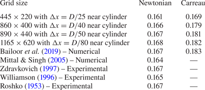
Table 2 reports the respective Strouhal numbers for Newtonian and shear-thinning fluids obtained using four different grid sizes, and compares them with the available literature data. Based on this observation, a grid size of  $D/50$ (near the cylinder) has been considered for all subsequent studies reported in this paper.
Strouhal numbers for flow past a stationary circular cylinder at  $Re = 100$.

3.1.2. Viscosity and vorticity contours
The time-averaged viscosity contour (in Pa s) in a Carreau fluid is shown in figure 6 for the flow over the stationary cylinder. The distribution of the viscosity is similar to the behaviour reported by Bailoor et al. (Reference Bailoor, Seo and Mittal2019). It is observed that the low-viscosity region is concentrated around the upstream stagnation point and in the wake region. On the other hand, the low-shear far-wake and free stream locations have nearly constant viscosity ( $\mu _{0}$). Low values of viscosity in the wake zone also result in a shorter formation length compared with that for the Newtonian fluid. Figure 7 shows an instantaneous distribution of vorticity. These observations are also similar to the results of Bailoor et al. (Reference Bailoor, Seo and Mittal2019).
Time-averaged viscosity contour for a Carreau fluid over a fixed cylinder.

Instantaneous vorticity contour for a Carreau fluid over a fixed cylinder.

3.2. Domain independence test
Three different domain sizes are considered with respective widths,  $H = 12D$,
 $16D$ and
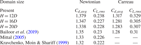
 $20D$. The flow features are apparently the same for all the domains for Newtonian and Carreau fluids. Average drag coefficient and r.m.s. of the lift coefficient are calculated for flow over the fixed cylinder and compared with the reported data in table 3. It can be noticed that for both Newtonian and Carreau fluids, mean and r.m.s. of the lift and drag coefficients for
 $H = 16D$ and
 $20D$ agree well with the available data. We consider the domain configuration with
 $H = 16D$ for performing all subsequent calculations. It should also be mentioned that force variations over the oscillating cylinder and the vortex patterns are also observed to be domain independent.
Lift and drag coefficients (average and r.m.s. values) for flow past a stationary circular cylinder at  $Re = 100$ with different domain sizes.

3.3. Investigations on the lock-in phenomena
Lock-in phenomena for the forced vibration of a cylinder in the uniform flow of a Newtonian fluid have been investigated in detail by a number of researchers (Bishop & Hassan Reference Bishop and Hassan1964; Koopmann Reference Koopmann1967; Karnidakis & Triantafyllou Reference Karnidakis and Triantafyllou1989). There have been certain discrepancies in the lock-in criterion proposed by different authors. To address this issue, Kumar et al. (Reference Kumar, Navrose and Mittal2016b) proposed an inclusive criterion based on the peak frequencies of the power spectrum of lift force. Accordingly, two conditions are checked:  $(a)$ the dominant frequency in the power spectrum of the lift coefficient is the same as the cylinder oscillation frequency and
 $(b)$ if any other peak frequencies are present in the power spectrum, they are integer multiples of the cylinder oscillation frequency. If both conditions are satisfied, the flow is categorized to be in the lock-in mode. If condition
 $(a)$ is satisfied but not
 $(b)$, the flow is said to be in the transition state. For all other cases, the system is considered to be in the non-lock-in state. We have attempted to identify the lock-in states for both Newtonian and Carreau fluids over a range of amplitudes and frequencies of the oscillation using this criterion. We also present the Lissajous phase to identify the lock-in phenomena with better clarity.
3.3.1. Lock-in behaviour with frequency variation
Earlier studies suggest that the lock-in phenomenon is observed when the oscillation frequency is close to the Strouhal frequency. So, to compare the lock-in behaviour in Newtonian and Carreau fluids, we have varied the frequency ratio as  $f^{*} = 0.6$,
 $0.8$,
 $1.0$ and
 $1.2$ while keeping the oscillation amplitude fixed to a moderate value (
 $A^{*}=0.4$). The power spectrum of the lift coefficient for these different cases is shown in figure 8. In all of these cases, we can observe a peak frequency at
 ${f}/{f_y}= 1.0$, which is the oscillation frequency of the cylinder. However, at a low-frequency ratio (
 $f^{*} = 0.6$), other peaks are observed at higher frequency which are not integer multiples of the oscillation frequency. At this low frequency and low-oscillation amplitude, the cylinder inertia effects are small and, therefore, the stationary vortex-shedding mode is dominant. The peak frequency is observed at
 ${f}/{f_y} = 0.167$, which is the same as
 ${f}/{f_{St}} = 1$ (as
 $f^{*}={f_y}/{f_{St}} = 0.6$ here). Consequently, this case corresponds to a non-locked-in case in both fluids. The moderate frequencies,
 $f^{*} = 0.8$ and
 $1.0$, correspond to locked-in cases with the only spectrum peak present at the oscillation frequency of the cylinder. At a further higher frequency,
 $f^*= 1.2$, smaller low-frequency peaks are observed near the main peak frequency (
 ${f}/{f_y} = 1.0$), which result in a departure from the lock-in behaviour. These fluctuations are more dominant in the Carreau fluids compared with the Newtonian case. We further look into the Lissajous pattern (figure 9) to discuss this departure.
Power spectrum of lift coefficient (PSD): (a,b)  $A^{*} = 0.4$ and
 $f^{*} = 0.6$; (c,d)
 $A^{*} = 0.4$ and
 $f^{*} = 0.8$; (e,f)
 $A^{*} = 0.4$ and
 $f^{*} = 1.0$; (g,h)
 $A^{*} = 0.4$ and
 $f^{*} = 1.2$, for (a,c,e,g) Newtonian (black line) and (b,d,f,h) Carreau fluids (red line).

Lissajous patterns – lift coefficient with the oscillation displacement of cylinder: (a)  $A^{*} = 0.4$ and
 $f^{*} = 0.6$; (b)
 $A^{*} = 0.4$ and
 $f^{*} = 0.8$; (c)
 $A^{*} = 0.4$ and
 $f^{*} = 1.0$; (d)
 $A^{*} = 0.4$ and
 $f^{*} = 1.2$, for Newtonian (black line) and Carreau fluids (red line).

In the cases with  $f^* = 0.8$ and
 $f^* = 1.0$, where a single dominant peak is observed at
 ${f}/{f_{St}} = 1.0$ and no peak is observed at a frequency lower than the oscillation frequency (figure 8c–f), the Lissajous patterns show a single curve indicating a constant phase difference between the cylinder displacement and lift force. The observations are similar for both Newtonian and Carreau fluids. These are the locked-in cases. At
 $f^* = 0.6$, both the fluids show higher frequency peaks in the lift spectrum and the Lissajous patterns show a non-repeating aperiodic behaviour and this is identified as a non-locked-in case for both the fluids. At higher oscillation frequency (
 $f^* = 1.2$), we observe small-amplitude noise near the main dominant peak at
 ${f}/{f_y} = 1.0$. The Lissajous plot for this case also reflects this departure from lock-in behaviour showing multiple lines instead of a single repeating curve. This non-lock-in behaviour is more pronounced in the Carreau fluid.
3.3.2. Lock-in behaviour with amplitude variation
At moderate-oscillation amplitude ( $A^{*} = 0.4$), both the fluids exhibit lock-in behaviour when the oscillation frequency matches (or is close to) the Strouhal frequency. Now, to investigate the lock-in behaviour for different amplitude ratios, we keep the oscillation frequency fixed at
 $f^{*} = 1.0$ and increase the amplitude. In figure 10, the power spectrum of the lift coefficient is presented for the amplitude ratios of 0.6, 1.0 and 1.2 with
 $f^*= {f_y}/{f_{St}} = 1.0$. The low-amplitude ratio case (
 $A^* = 0.6$) presents a single dominant peak at
 ${f}/{f_y} = 1.0$ indicating locked-in flow. At a higher amplitude ratio,
 $A^* = 1.0$, the Carreau fluid shows another peak at
 ${f}/{f_y} = 3.0$, which is an integer multiple of the peak dominant frequency, so this case is still locked-in. However, at an even higher amplitude ratio (
 $A^* = 1.2$), the dominant peak in the Carreau fluid is still at
 ${f}/{f_y} = 3.0$. This clearly shows a deviation from the locked-in mode as per criterion (a) discussed above. For Newtonian fluids, although peaks are visible at higher frequencies, the dominant frequency is still at
 ${f}/{f_y} = 1.0$ satisfying the lock-in criteria. The Lissajous patterns in figure 11 also confirm these observations.
Power spectrum of lift coefficient (PSD): (a,b)  $A^{*} = 0.6$ and
 $f^{*} = 1.0$; (c,d)
 $A^{*} = 1.0$ and
 $f^{*} = 1.0$; and (e,f)
 $A^{*} = 1.2$ and
 $f^{*} = 1.0$, for (a,c,e) Newtonian (black line) and (b,d,f) Carreau fluids (red line).

Lissajous patterns – lift coefficient with the oscillation displacement of cylinder: (a)  $A^{*} = 0.6$ and
 $f^{*} = 1.0$; (b)
 $A^{*} = 1.0$ and
 $f^{*} = 1.0$; and (c)
 $A^{*} = 1.2$ and
 $f^{*} = 1.0$, for Newtonian (black line) and Carreau fluids (red line).

We can infer that at  $f^{*}=1.0$, the lock-in behaviour is similar for both Newtonian and Carreau fluids up to
 $A^*=1.0$, except for minor deviations. However, as the amplitude ratio increases to
 $A^* = 1.2$, Newtonian fluid shows lock-in behaviour but the Carreau fluid behaves differently.
3.3.3. Variation in drag coefficient
figure 12 shows variation in the drag forces during different oscillation cycles. We can observe that the locked-in cases in figure 12(b,c) show synchronized behaviour of the drag variation with a frequency twice that of the oscillation frequency for both Carreau and Newtonian fluids. However, the non-locked-in case (figure 12a) shows aperiodic variation of the drag coefficient. Figure 12(d) shows a variation in drag coefficient for  $A^{*} = 1.2$ and
 $f^{*} = 1.0$ for both fluids. The Newtonian fluid shows periodic variation with a constant peak amplitude over different cycles. However, for the Carreau fluid, different peak values of
 $C_d$ are observed during the oscillation cycle as this is a non-locked-in case. It should be mentioned that the cycle-averaged drag coefficients are slightly smaller in the Carreau fluid compared with the Newtonian fluid (table 4).
Variation in drag coefficient during cylinder oscillation: (a)  $A^* = 0.4\ {\rm and}\ \,f^* = 0.6$; (b)
 $A^* = 0.4\ {\rm and}\ \,f^* = 1.0$; (c)
 $A^* = 1.0\ {\rm and}\ \,f^* = 1.0$; and (d)
 $A^* = 1.2\ {\rm and}\ \,f^* = 1.0$.

Average drag coefficient ( $C_{d,avg}$).

It is well known that the lock-in behaviour results from the synchronization of the vortex shedding with the cylinder oscillation cycle (Barbi et al. Reference Barbi, Favier, Maresca and Telionis1986; Yokoi & Kamemoto Reference Yokoi and Kamemoto1994). In the following sections, we investigate the vortex dynamics for different oscillation cases and try to observe the differences in the behaviour of Newtonian and Carreau fluids, especially at the higher oscillation amplitudes.
3.4. Vortex dynamics for different oscillation cases
Figure 13 presents the lock-in and non-lock-in modes in a  $f^*-A^*$ map for both Newtonian and Carreau (
 $Cu=1.0$,
 $n=0.25$) fluids along with their respective vortex advection patterns. We can observe that the low- or moderate-amplitude locked-in cases result in synchronized 2S vortices. In these cases, the vortex pattern is similar for both the fluids with some differences in peak vorticity and vortex wavelengths (discussed in later subsections). Furthermore, in the non-lock-in cases at extreme frequencies (
 $\,f^*=0.6$ and 1.2) at
 $A^*=0.4$, we can observe the formation of pair vortices (P) in both the fluids. However, for the high-amplitude oscillation case (
 $A^*=1.2, f^*=1.0$) both fluids show a P+S mode, though the flow structures are substantially different. Vortices generated in the Carreau-fluid case show stronger asymmetry compared with the Newtonian-fluid case. This case also shows different lock-in behaviour in different fluids. We seek to understand these differences in more detail in a later subsection.
Lock-in behaviour and vortex modes for Carreau ( $Cu=1.0$,
 $n=0.25$) and Newtonian fluids over different amplitude and frequency ratios (cylinder is in the mean position).

3.4.1. Vortex dynamics of 2S mode during lock-in oscillation
The 2S-mode vortex dynamics is qualitatively similar in the Newtonian and Carreau fluids. Here, the shedding of two single (2S) vortices is synchronized with the oscillation cycle. In figure 14, we show vortex contours at different phases of an oscillation cycle for a Newtonian fluid at  $f^* = 1.2$,
 $A^* = 0.4$. It should be mentioned that similar patterns of vortex motion are observed for all locked-in 2S-mode cases for both Newtonian and Carreau fluids. In figure 14, two predominant vortical regions, the positive shear layer (PS layer) and the negative shear layer (NS layer) can be observed along with a minor arc base region vorticity (ABRV) on the cylinder surface. The vorticity dynamics after the separation point is largely governed by the interaction of the ABRV with the shear layers present at the upper and lower surfaces of the cylinder (Krishnan et al. Reference Krishnan, Agrawal, Sharma and Sheridan2016, Reference Krishnan, Agrawal, Sharma, Thompson and Sheridan2019). Figure 14 depicts the growth and decay of the positive and negative ABRVs for a complete oscillation cycle.
Vorticity dynamics of the 2S mode – snapshots of vortex contours over a complete oscillation cycle ( $f^*=0.8, A^*=0.4$, Newtonian fluid). PABRV, positive signed arc base region vorticity; NABRV, negative signed arc base region vorticity; PS layer, positive shear layer; and NS layer, negative shear layer. The growth and decay of PABRV are shown in circles in panels (a–d,i), while the growth and decay of NABRV are shown in circles in panels (e–h). Vorticity scale is the same as that in figure 13.

At the beginning of the present cycle, PABRV is observed over the cylinder surface (wake side), which grows further in the subsequent phases and reaches a peak (figure 14a–c) and then decays (figure 14d). Through these steps, it feeds vorticity to the lower PS layer and the PS layer undergoes a stretching. Note that the growth and the decay of PABRV and stretching of the PS layer are also associated with the movement of the NS layer. The NS layer weakens by the growth of PABRV and it breaks down to form an S vortex during this phase. The mechanism of vortex shedding arising from activities of the base region vorticity is discussed in detail by Krishnan et al. (Reference Krishnan, Agrawal, Sharma, Thompson and Sheridan2019) for flow past a square cylinder. In the next half of the cycle, a NABRV is observed which results in the formation of the other S vortex. The mode of vortex shedding is similar in Carreau fluids.
The locations of the vortex cores are identified using the  $Q$-criterion. Hunt, Wray & Moin (Reference Hunt, Wray and Moin1988) formulated the criterion for identification of vortices in an incompressible flow. Here,
 $Q = (\|\varOmega \|^2 - \|S\|^2)/2$ is a measure of the local rotation rate in excess of the strain rate. When
 $Q > 0$, the vortex is identified as a region where there is more rotation than straining. Figure 15 shows the location of the vortices as observed using the
 $Q$-criterion and maximum vorticity magnitude for all 2S-mode cases. The distance between two consecutive vortex cores is measured as half of the vortex wavelength, as marked in figure 15. This wavelength is nearly constant for a particular flow case over the passage of vortices. The Carreau fluid shows a 4–10 % shorter wavelength than the Newtonian fluid. This can be attributed to the fact that the shear-thinning nature of Carreau fluids reduce the viscosity near the vortices and therefore restricts their diffusion.
Vorticity and  $Q$-criterion contour for Newtonian and Carreau fluids at different amplitudes and frequencies. Vortex cores are shown with a maximum peak of the
 $Q$-criteria contour. Inner vortex separation lengths are also shown. (a)
 $A^{*} = 0.4, f^{*} = 0.8$; (b)
 $A^{*} = 0.4, f^{*} = 1.0$; (c)
 $A^{*} = 0.6, f^{*} = 1.0$; and (d)
 $A^{*} = 1.0, f^{*} = 1.0$.

3.4.2. Vortex dynamics for non-locked-in-mode formation of a pair of vortices
Figure 16 shows the formation and advection of vortices in the strongly non-locked-in case ( $A^{*}=0.4, f^{*}=0.6$). The flow structures show consecutive shedding of the single (S) and pair (P) vortices but the vortex-shedding cycle does not synchronize with the cylinder oscillation cycle. The pattern of P and S vortices are similar for both the Newtonian and Carreau fluids. However, the inner vortex separation lengths are shorter for the Carreau fluid. It is important to observe that the ABRV does not show periodicity over a complete oscillation cycle. A combined ABRV (CABRV) is observed, where both positive and negative vorticities exist simultaneously at the cylinder arc base. Owing to the non-synchronization of the growth and decay of ABRV with cylinder oscillation, the variation of lift force does not synchronize with the cylinder oscillation cycle. Hence, this oscillation shows a non-lock-in mode. Formation of CABRV is also observed in the non-locked-in case with
 $A^*=0.4, f^*=1.2$, where 2P vortices are observed in both fluids. However, the smaller values of wake-region viscosity in Carreau fluids result in a shorter vortex formation length and introduces higher levels of fluctuations.
Vorticity contours during  $A^{*} = 0.4, f^{*} = 0.6$ oscillation cycle for Newtonian and Carreau fluids.

3.4.3. Vortex dynamics of (P+S) mode –  $f^* = 1.0$, $A^* = 1.2$


Oscillations with  $A^* = 1.2$,
 $f^* = 1.0$ show a P+S vortex mode in both fluids. Interestingly, this high-amplitude oscillation is the only case in our investigation in which the Newtonian fluid shows lock-in behaviour but the Carreau fluid behaves differently (figure 11c). Figure 17 shows that in the first half of the cycle, P vortices are advected and the later half sheds an S vortex. The vortex patterns in Newtonian and Carreau fluids are visibly different in this oscillation cycle. The Newtonian fluid shows a connected region of negative vorticity joining the S vortex with the negative vortex of the P pair (figure 17b). The S vortices in the Newtonian fluid are weaker and strained. A
 $Q$-criteria-based visualization also helps us to identify these vortices distinctively (figure 18). In the Carreau fluid, the vortices are discrete and follow a strong asymmetric pattern. The Carreau fluid vortices are stronger and they orient themselves quickly along the flow direction as they move downstream. The fast Fourier transformation (FFT) of the downstream location streamwise velocity is also presented (figure 19). In the Newtonian fluid, we can see that the peak frequency is twice that of the oscillation frequency, which indicates the advection of P and S vortices during one complete oscillation cycle. In the Carreau fluid, FFT shows multiple harmonics with a higher level of unsteadiness. The formation of S and P vortices as well as the breaking down of the negatively connected region of vorticity (one S and one of the P pair) are reflected by this signal. This activity further contributes to the fluctuations in the lift force (figure 11c) and sets in the no-lock-in behaviour.
Vorticity contours during an  $A^{*} = 1.2, f^{*} = 1.0$ oscillation cycle for Newtonian and Carreau fluids.

 $Q$-criterion map to locate the vortex cores in the
 $A^{*}=1.2, f^{*}=1.0$ case.

FFT of streamwise velocity in the wake region for  $A^{*}=1.2, f^{*}=1.0$ Newtonian (a) and Carreau (b) fluids.

The ABRV shows an interesting behaviour for this case (figure 17). We can see that both the positive and negative ABRV are aligned with the cylinder surface near the bottom (or top) half of the cylinder during its upward (or downward) motion. The formation of ABRV in this location on the cylinder surface arises from the higher acceleration of the cylinder in this oscillation cycle. Pressure contour and streamline maps show a low-pressure region at this location and a saddle point in its vicinity (figure 20). The low-pressure zone is wider in the Newtonian fluid while disconnected and stronger negative pressure regions are visible during the motion of the Carreau fluid. The pressure distribution reflects the differences in the vortex patterns in these two fluids. We will try to explain this behaviour through the vorticity transport equation in a later subsection.
Pressure contour and streamlines for  $A^{*}=1.2, f^{*}=1.0$ Newtonian (a) and Carreau (b) fluids.

3.5. Relation of arc base region vorticity and the vortex modes
Following the discussions in the previous section, we can attribute the features of the vortex motion in flow past an oscillating cylinder to two key factors: (i) the behaviour of ABRV, which is responsible for the formation of the S or P vortices; and (ii) the viscous diffusion, which governs the spreading of the vortices in the downstream region. The formation of the vortices is largely governed by the interaction of the ABRV with the streamwise shear layers. For the locked-in cases, the PABRV interacts with the negative shear layer and forms a negative S vortex during the first half of the cycle. In the next half, a positive S vortex is formed similarly. The non-locked-in cases show formation of P vortices. These vortices arise from the formation of CABRV. When these combined vortices show an overlapping pattern, i.e. the PABRV forms an envelop for the NABRV (which is attached to the cylinder surface), both the vortices simultaneously cut the PS and NS layers and form a P vortex. In the other case, where both the positive and negative ABRV are side by side aligned over the cylinder surface, a P vortex is formed during the first half of the cycle and an S vortex is formed in the next half. This behaviour, listed in table 5, is similar in both the Newtonian and Carreau fluids.
Effects of arc base region vorticity on vortex shedding.

3.6. Generation of vorticity during oscillation cycles and enstrophy
Vortex patterns near the cylinder surface are independent of the rheology of the fluid (Newtonian or Carreau). However, these patterns, as well as the formation of ABRVs, are strongly related with the cylinder motion. Therefore, it will be useful to find a relation between the cylinder motion and the generation of vorticity on the cylinder surface. In a 2-D flow, the vorticity flux from a curved surface (where  $n$ is the surface normal coordinate) can be defined as
 \begin{equation} \sigma_z = \frac{\partial \omega_z}{\partial n}. \end{equation}
Here,  $\sigma _{z}$ is the measure of the amount of vorticity that is entering the flow from the solid walls. Now, using the momentum equations, the vorticity gradient can be related to the pressure gradient on the surface of a stationary object (where
 $\boldsymbol {V} = 0$) and the vorticity flux can be obtained as
 \begin{equation} \frac{\partial p}{\partial s} = \mu \frac{\partial \omega_z}{\partial n} = \mu \sigma_z, \end{equation}
where  $s$ is the coordinate along the surface tangent. Further, for an accelerating surface, the local inertia force augments the vorticity flux as
 \begin{equation} \mu \sigma_z = \frac{\partial p}{\partial s} + \rho a_s, \end{equation}
where  $a_s$ is the tangential acceleration of the surface.
Proof of the above relation may be found in the paper by Panton (Reference Panton2013). Therefore, the influx of vorticity from the cylinder wall is a function of the surface pressure gradient and the tangential component of the cylinder acceleration. Coelho & Pinho (Reference Coelho and Pinho2004) showed that for flow over fixed cylinders, the pressure gradient in a shear-thinning flow is moderately higher than that in a Newtonian flow. Also, the non-zero values of the pressure gradient are mostly restricted within the minimum pressure point and base pressure region on the wake side of the cylinder. However, as the viscosity of the Carreau fluid reduces near the solid wall, owing to higher strain rates, the vorticity flux increases as per (3.2) and (3.3) respectively for the fixed and oscillating cylinder. Consequently, non-Newtonian shear-thinning fluids show higher vorticity values in the vicinity of the cylinder (observed by Chhabra et al. (Reference Chhabra, Soares and Ferreira2004) and Bharti et al. (Reference Bharti, Chhabra and Eswaran2007) for fixed cylinders) compared with Newtonian fluids. For moving cylinders, this difference is further enhanced when the cylinder acceleration is high ((3.3)). So, the vorticity formation patterns remain similar for both the fluids but the magnitude of vorticity is higher in a Carreau fluid.
Enstrophy for this 2-D flow is obtained as
 \begin{equation} E = \int_{A} \omega_{z}^{2} \,\textrm{d}A. \end{equation}
Enstrophy is proportional to the total rotational energy of the vortices in the flow. The higher influx of vorticity ( $\sigma _z$), in the case of Carreau fluids, results in higher levels of enstrophy of the flow. Figure 21 presents the enstrophy variation during the oscillation cycles for both Newtonian and Carreau fluids. Apart from the strongly non-locked-in case in figure 21(a) (
 $f^* = 0.6$,
 $A^* = 0.4$), enstrophy shows a periodic behaviour for both Newtonian and Carreau fluids. However, its magnitude is higher for Carreau fluids owing to the lower value of viscosity. It is also important to mention here that we have obtained a 20–30% reduction of the average viscosity in the Carreau fluid compared with the Newtonian fluid over all the oscillation cases. At higher oscillation frequency and amplitude, the enstrophy increases for both Newtonian and Carreau fluids as the vorticity flux increases owing to the cylinder acceleration ((3.3)). During a sinusoidal cylinder oscillation cycle, the magnitude of the acceleration attains a maximum value twice and results in the two peaks in the enstrophy plots. A full cycle of growth and decay of both the positive and negative ABRVs are observed during a complete oscillation cycle for all these cases except for the low-frequency low-amplitude non-locked-in case. In this case, the vorticity flux is mostly governed by the pressure gradient (owing to lower levels of cylinder acceleration) and thus is not forced to follow the oscillation cycle.
Enstrophy fluctuation during cylinder oscillation cycles for Newtonian (black line) and Carreau fluids (red line): (a)  $A^{*} = 0.4, f^{*} = 0.6$; (b)
 $A^{*} = 0.4, f^{*} = 1.0$; (c)
 $A^{*} = 1.0, f^{*} = 1.0$; and (d)
 $A^{*} = 1.2, f^{*} = 1.0$.

3.7. Vorticity transport rate analysis
Figure 22 shows the snapshots of viscosity contours of the Carreau fluid at the mean location of the cylinder during its course of upward motion for the different oscillation cases. It can be seen that the viscosity levels are lower in the vicinity of the cylinder, especially at the wake zone. The primary shear layers and the arc base region vortices show almost a 50 % reduced viscosity. Lower levels of viscosity are also found near the vortex cores.
Viscosity contours for different oscillation cases in a Carreau fluid: (a)  $A^{*} = 0.4, f^{*} = 0.6$; (b)
 $A^{*} = 0.4, f^{*} = 1.0$; (c)
 $A^{*} = 1.0, f^{*} = 1.0$; and (d)
 $A^{*} = 1.2, f^{*} = 1.0$.

While the smaller levels of viscosity in a Carreau fluid are responsible for higher vorticity generation near the cylinder wall and smaller inner separation length at the wake zone (figure 15), it should be noted that the patterns of vortex formation and advection of vortices do not show much difference from the Newtonian flow behaviour in most of the cases considered. (The supplementary movies 1–4 and 6–9 available at https://doi.org/10.1017/jfm.2021.485 are related to figures 22 and 23, showing the variations in viscosity and vorticity during the cylinder oscillation cycles.)
Contours of  ${\textrm {D}\omega _z}/{\textrm {D}t}$ for different oscillation cases – (a,c,e,g) Newtonian, (b,d,f,h) Carreau fluids: (a,b)
 $A^{*} = 0.4, f^{*} = 0.6$; (c,d)
 $A^{*} = 0.4, f^{*} = 1.0$; (e,f)
 $A^{*} = 1.0, f^{*} = 1.0$; and (g,h)
 $A^{*} = 1.2, f^{*} = 1.0$.

To understand the advection pattern and breaking of the vortices, we look into the vorticity transport equation ((3.5)):
 \begin{equation} \frac{\textrm{D}\omega_z}{\textrm{D}t} = \boldsymbol{\nabla} \boldsymbol{\cdot} (\eta (|\boldsymbol{\dot{\gamma}}|)\boldsymbol{\nabla} \omega_z) + \boldsymbol{\nabla} \boldsymbol{\cdot} f,\end{equation}
where  $\eta (|\boldsymbol {\dot {\gamma }}|$ is the non-Newtonian kinematic viscosity and
 $f$ represents the non-Newtonian viscosity gradient term and is given as
 \begin{equation} f = \begin{bmatrix}
\dfrac{\partial \eta|\boldsymbol{\dot{\gamma}}|}{\partial
x} \left(\dfrac{\partial u}{\partial y} +\dfrac{\partial
v}{\partial x}\right) -2\dfrac{\partial
\eta|\boldsymbol{\dot{\gamma}}|}{\partial y}\dfrac{\partial
u}{\partial x}\\ \dfrac{\partial
\eta|\boldsymbol{\dot{\gamma}}|}{\partial y}
\left(\dfrac{\partial u}{\partial y} +\dfrac{\partial
v}{\partial x}\right) -2\dfrac{\partial
\eta|\boldsymbol{\dot{\gamma}}|}{\partial x}\dfrac{\partial
v}{\partial y} \end{bmatrix} .
\end{equation}
As the flow is 2-D, only the  $z$-component of vorticity and the
 $x$,
 $y$ components of velocity and co-ordinate are considered. This is to note that for the Newtonian fluid, kinematic viscosity is constant,
 $\eta$, and the vorticity transport equation is simply written as
 \begin{equation} \frac{\textrm{D}\omega_z}{\textrm{D}t} = \eta \nabla^2 \omega_z \end{equation}
In (3.5) and (3.7), the vorticity transport rate (VTR),  ${\textrm {D}\omega _z}/{\textrm {D}t}$, is balanced by the net viscous diffusion of vorticity and it represents the rate of net growth and advection of the vorticity. For the Carreau fluids, we can express the right-hand side of (3.5) as a combination of viscosity multiplied by the Laplacian of vorticity (as in (3.7)) and another extra term owing to the gradients of non-Newtonian viscosity denoted as NN terms:
 \begin{equation}
\frac{\textrm{D}\omega_z}{\textrm{D}z} =
\underset{{term\ I}}{\underbrace{\eta (
|\boldsymbol{\dot{\gamma}}|) \varDelta^2\omega_z}} +
\underset{{term\ II}}{\underbrace{{NN\ terms}}}.
\end{equation}
In figure 23, we present the contours of VTR ( ${\textrm {D}\omega _z}/{\textrm {D}t}$) for Newtonian and Carreau fluids, respectively as obtained as the right-hand side of (3.7) and (3.8). It can be seen that the primary shear layers and ABRV show peaks of VTR for both the fluids owing to the high-vorticity gradients at these regions. However, the magnitudes of these VTR peaks (both positive and negative values) are higher in a Carreau fluid. In these cases, the high values of VTRs sharply reduce to smaller levels. Also, for high-frequency and high-amplitude cases (figure 23(b,d,f,h)) in a Carreau fluid, high-VTR zones are less spread in the streamwise direction. The case of
 $A^* = 1.2$,
 $f^* = 1.0$ is of particular interest here. At this oscillation cycle, both the fluids show P+S modes though the Newtonian fluid shows a connection between one of the P vortices and the S vortex but the Carreau fluid shows distinct strong vortices (figure 17). In figure 23(g,h), a higher rate of positive viscous diffusion of vorticity (or VTR) is observed between the P and S vortices in the Carreau fluid case. Owing to this high diffusion rate, the negative vorticity region between the P and S vortex (as shown in figure 19) diffuses quickly and distinct vortices are advected downstream.
For the Carreau fluid, the viscosity is a strong function of strain rate, and hence, the second term in (3.8) is related to the local strain rates. Therefore, the viscous diffusion for a Carreau fluid is augmented owing to the higher levels of local straining although viscosity can be of reduced magnitude at these regions. To quantify the relative contribution of both the components of viscous diffusion (term I and term II from (3.8)), we propose a correlation function:
 \begin{equation} \varOmega_c
=
\frac{4\times {term\ I} \times {term\
II}}{({term\ I}+ {term\ II})^2}.
\end{equation}
If both the terms are equal, then this correlation,  $\varOmega _c$, reaches a maximum value of unity. If both the terms are of opposite sign, then it shows a negative value. A high-negative value of
 $\varOmega _c$ implies that even when the individual terms are high, they are of opposite sign and hence they cancel each other, and the net viscous diffusion (or VTR) is small. Now, we compute
 $\varOmega _c$ for different oscillation cases of the Carreau fluid and present the instantaneous contours in figure 24. It should be mentioned that when both the terms are very small (
 ${<}0.05$), the correlation value is clipped to zero for smoothness. Figure 24 identifies the zones with higher (
 ${>}0.5$) and lower (
 $<= -1$) values of
 $\varOmega _c$. The side-by-side appearance of these two zones explains the high value of VTR (owing to same-signed values of both the terms) and its sharp drop (owing to opposite-signed comparable values of the terms). The negative values of
 $\varOmega _c$ obtained near the vortex cores (figure 24b,d) results in reduction of the viscous diffusion and the vortices retain their strength during advection downstream. In contrast, the decay of Newtonian vortices is much faster owing to a higher viscous diffusion. Also, the negative
 $\varOmega _c$ region is restricted mainly in the close vicinity of the vortex cores in the
 $A^* = 1.2$,
 $f^* = 1.0$ case. Therefore, the diffusion between the vortices is higher (as observed in figure 24d) and results in the formation asymmetric P+S vortices in Carreau fluids.
Contours of  $\varOmega _{c}$ for different oscillation cases in a Carreau fluid: (a)
 $A^{*} = 0.4, f^{*} = 0.6$; (b)
 $A^{*} = 0.4, f^{*} = 1.0$; (c)
 $A^{*} = 1.0, f^{*} = 1.0$; and (d)
 $A^{*} = 1.2, f^{*} = 1.0$.

3.8. Effect of Carreau fluid properties
Here, we present investigations on the effect of Carreau number ( $Cu$) and power index (
 $n$) on the flow behaviour. The lock-in behaviour and vortex patterns are found to be similar over a range of Carreau fluid properties:
 $Cu = 1, 10$ and
 $n = 0.25, 0.5$. However, we can notice quantitative differences in terms of inner vortex separation lengths as shown in figure 25 for
 $A^* = 0.4$,
 $f^* = 1.0$. We can observe that the distance between the vortices reduce with smaller
 $n$ and higher
 $Cu$ values. However, the effect of
 $n$ is smaller at higher
 $Cu$. It should be mentioned that Pantokratoras (Reference Pantokratoras2016) observed that flow properties do not show much variation with respect to power index at higher
 $Cu$ for
 $Re > 40$. Nevertheless, the viscosity contours show strong sensitivity to
 $Cu$ and the wake region shows smaller viscosity levels at
 $Cu = 10$ (figure 26a). It can be inferred that the smaller viscosity in the wake region results in higher levels of vorticity near the vortex cores for
 $Cu = 10$ (figure 25). However, we can further observe that the vorticity transport rate is of same order for both Carreau numbers (figure 26b) and as a result of this, the vortex patterns are also similar in these two cases. We further inform that this similarity is observed in all oscillation cases for these different sets of
 $Cu$ and
 $n$ values (the supplementary movies 2, 5, 7 and 10 in the supplementary material are related to figure 26).
Vorticity contours for different  $Cu$ and
 $n$ values with
 $A^{*} = 0.4, f^{*} = 1.0$.

(a,b) Viscosity contours and (c,d) VTR for different  $Cu$ with
 $n = 0.25$ and
 $A^{*} = 0.4, f^{*} = 1.0$.

4. Conclusion
Numerical simulations are performed to compare the lock-in phenomena and vortex patterns in flow over transversely oscillating cylinders in shear-thinning Carreau and Newtonian fluids. The sharp-interface immersed boundary method is used to model the oscillating cylinder in the background of a rectilinear mesh. A range of oscillation amplitudes and frequencies is studied. It is observed that the lock-in behaviour is mostly similar for both the fluids except for the high-amplitude case ( $A^{*} = 1.2, f^{*} = 1.0$), where the vortex patterns are visibly different in these two fluids. Although both fluids show the P+S vortex-shedding mode, the Carreau fluid vortices show a stronger asymmetric pattern with higher levels of unsteadiness and thus depart from the lock-in mode. In all other cases, the vortex patterns are similar. The lock-in modes show symmetric S vortex shedding for both the fluids. However, the vortex separation length is shorter in the Carreau fluid owing to a smaller viscous diffusion in the wake zone. The mechanism of vortex formation is explained via the behaviour of the base region vorticity. It is also observed that the vorticity generation mechanism is similar in both the fluids and it is largely governed by the cylinder acceleration except for the low-frequency low-amplitude case (
 $A^*=0.4$,
 $f^*=0.6$). However, the magnitude of vorticity is higher in Carreau fluids as the viscosity is of reduced order (nearly 50
 $\%$ smaller than
 $\mu _0$ for
 $Cu=1.0$,
 $n=0.25$) near the cylinder surface. We observed that the vortex-shedding modes are governed by the dynamics of the base region vorticity for both fluids. The patterns of advection of the wake vortices are further explained through the vorticity transport equation. In Carreau fluids, an extra term arises in the vorticity transport equation owing to the gradients of viscosity. Correlation of this term with the vorticity Laplacian is computed. We observed that a negative correlation between these two terms results in smaller viscous diffusion and advection of stronger vortices in Carreau fluids. However, for
 $A^{*} = 1.2, f = 1.0$, these two terms show a positive correlation in the near-cylinder wake region and the enhanced diffusion results in the formation of stronger distinct vortices in the Carreau fluid yielding a vortex pattern different from that in a Newtonian fluid. We observed differences in the wake region viscosity for different Carreau fluids. However, the vortex patterns and the lock-in behaviour are similar for these fluids as they exhibit similar variation in vorticity transport rates.
This study has been one of the first attempts to understand non-Newtonian fluid mechanics for flow past oscillating cylinders. Further investigation over a range of Reynolds numbers, geometric parameters, oscillating behaviours and so forth can unveil the distinct flow features in the dynamics of shear-thinning fluid dynamics over accelerating objects.
Supplementary movies
Supplementary movies are available at https://doi.org/10.1017/jfm.2021.485.
Acknowledgements
Paramshakti, a super-computing facility at IIT Kharagpur established through National Super Computing Mission, Government of India, has been used for this research.
Funding
The authors acknowledge financial support through IIT Kharagpur ISIRD grant (project code: ODC).
Declaration of interests
The authors report no conflict of interest.