





1. Introduction
The oscillating water column (OWC) concept (see Heath Reference Heath2012; Falcão & Henriques Reference Falcão and Henriques2016, for example) is, to date, arguably the most commercially successful device for converting ocean wave energy into electricity. Originally devised by Yoshio Masuda in the 1940s as a means of powering floating navigation buoys (see Masuda Reference Masuda1985), a number of modestly sized plants have been installed in a variety of settings and operated with some success, supplying energy to national electrical grids. For a recent review, see Gayathri et al. (Reference Gayathri, Chang, Tsai and Hsu2024).
Oscillating water columns operate by isolating an internal air chamber from the open ocean via a surface-piercing lip with an opening below the water line. The rise and fall of incoming waves forces the enclosed air above the internal free surface back and forth through an air turbine whose role is to generate electrical energy. A self-rectifying turbine, such as a Wells turbine (described in Falcão & Henriques Reference Falcão and Henriques2016), is typically used; it is designed to spin in the same direction regardless of the direction of the air flow. The success of the OWC lies in its simplicity: the only moving part is the air turbine, located above the water line. Being typically mounted at the shoreline mitigates the expense and difficulty of mooring, power transmission and maintenance operations associated with offshore wave energy devices. On the other hand, shore-mounted OWCs such as Kvaerner in Norway (see Falnes Reference Falnes1993), the pilot plants of PICO in the Azores (see Falcão et al. Reference Falcão, Sarmento, Gato and Brito-Melo2020) and LIMPET on the Scottish Island of Islay (see Boake et al. Reference Boake, Whittaker, Folley and Hamish2002) are considered difficult to build with site-specific constraints and a significant environmental impact. Additionally, the nearshore wave energy resource is not as high as far offshore whilst being more vulnerable to violent wave breaking events. Projects in Japan, India, China, Italy and Spain have involved installing OWC units into sea walls to serve a dual purpose of coastal/harbour protection and energy generation. To date, the largest and most successful of these is the Mutriku Wave Power Plant on the northern coast of Spain. It comprises 16 OWCs set side-by-side in a harbour wall, rated at 296 kW, and has been in operation since 2011. It has since supplied over 3 GWh to the grid (see Lopez-Mendia et al. Reference Lopez-Mendia, Aristondo, Ricci, Lekube, Ceballos and Robles2025).
It was the during the initial surge in interest in wave energy in the response to the oil crisis of 1973 that the theoretical basis for the operation of wave energy converters, including OWCs, was established (for an overview see Evans Reference Evans1981). Early, but instructive, work on the OWC concept by Evans (Reference Evans1978) applied rigid-body theory to a simple OWC model. By modelling the internal free surface as a weightless piston, it was demonstrated that the resonant motion of the fluid within the internal chamber can be excited at certain incident wave frequencies dependent on the depth of submergence of the duct. Shortly afterwards, Falcão & Sarmento (Reference Falcão and Sarmento1980) correctly accounted for the internal free surface using a theory based on oscillating pressure variations within the air chamber of the OWC device. This led to the general theoretical framework for multiple interacting OWCs described by Evans (Reference Evans1982) and Falnes & McIver (Reference Falnes and McIver1985). Some years later Evans & Porter (Reference Evans and Porter1995), revisiting a problem initially considered by Smith (Reference Smith1983), showed how a simple two-dimensional model of a shore-mounted OWC could extract 100 % of the incoming wave energy at an isolated resonant frequency dependent on the size and shape of the submerged rectangular chamber. In Evans & Porter (Reference Evans and Porter1995) only curves showing the maximum theoretical efficiency were shown whilst the effect of air compressibility was overlooked, although it is not difficult to extend their analysis and results to include these effects.
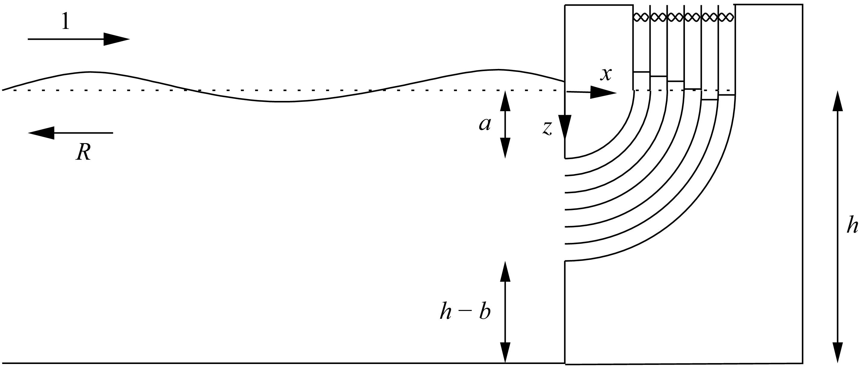
The modelling of OWCs has advanced over the last 30 years and many theoretical studies have been made of more complex OWC geometries in more realistic three-dimensional settings including arrays of devices. See, for example, Martin-Rivas & Mei (Reference Martin-Rivas and Mei2009), Zheng et al. (Reference Zheng, Antonini, Zhang, Greaves, Miles and Iglesias2019) and references therein. In this paper we return to the simpler two-dimensional setting in order to assess how a shift in fundamental OWC design affects its performance. A submerged opening is connected to an internal free surface via an annular duct which is divided into
 $N$
(we suppose many) separate narrow annular channels with thin, rigid, curved baffles. The air enclosed above each narrow channel is connected to the atmosphere via its own Wells turbine. The idea of the design is to broaden the device response. Since there are
 $N$
channels of different lengths, the proposed device possesses resonances at
 $N$
closely spaced frequencies, the largest/smallest of which are associated with the shortest/longest channels within the array.
The idea of engineering multiple resonant frequencies within a single device is not new. For example, the Belfast OWC concept of the 1970s (see Whittaker et al. Reference Whittaker, Leitch, Long and Murray1985) had two chambers tuned to two different frequencies housed within a circular device. The Kvaerner device described by Falnes (Reference Falnes1993) was unique in that it was built into a natural harbour to couple harbour resonance with device resonance. Closely related to the current proposal, Wilks et al. (Reference Wilks, Montiel and Wakes2022) considered a theoretical two-dimensional concept comprising multiple vertical channels of gradually increasing submerged depth separated by thin vertical baffles. The oscillations of the fluid powered rigid pistons placed on the surface of each channel and it was shown that efficiency close to 100 % across a broad range of frequencies could be achieved. The design of Wilks et al. (Reference Wilks, Montiel and Wakes2022) was guided as much by the principle of graded arrays and so-called rainbow reflection (the slowing of effective wave speed) as it was by multiple resonance. Very recently, Hu et al. (Reference Hu, Cheng, Dai, Yuan and Inececik2025) have considered the modification of the Wilks et al. (Reference Wilks, Montiel and Wakes2022) proposal, where rigid pistons are replaced by OWC chambers. In their work, 5 vertical channels of increasing immersed depth are considered using computational fluid dynamics simulations which include turbulent effects and air compressibility, whilst the incoming waves propagate from a model energy density spectrum. Despite turbulent losses caused by flow separation around the sharp edges of the thin vertical barriers, the authors report a broadband efficiency of more than 50 % over the range of resonant frequencies.
The OWC device described in this paper is really a closely packed system of
 $N$
coupled OWC devices, and so formally the general theory of Evans (Reference Evans1982) applies. However, a different approach is taken here, one which has proved successful in other application areas (see, for example, Zheng et al. Reference Zheng, Porter and Greaves2020; Huang & Porter Reference Huang and Porter2023). The geometric complexity of the baffle-partitioned duct is replaced with an effective medium using asymptotic homogenisation. This process is described in § 2 of the paper in the midst of the formulation of the problem and its solution. It formally applies for
 $N \gg 1$
, but in other problems has been shown to provide a good approximation to the geometrically exact solution, provided the length to width ratio of the channels is sufficiently large (roughly a factor of 10). See, for example, Liang et al. (Reference Liang, Porter and Zheng2024), who considered plane wave scattering parallel arrays of thin closely spaced plates. In § 2 it is shown how this simplification allows the problem to be reduced to a single scalar integral equation solution. This is approximated numerically, in § 4 of the paper, using Galerkin’s method. Two expressions for the efficiency of power capture are derived in § 3, one based on power capture at the device and one based on a far-field energy flux calculation. These lead to independent numerical methods for computing the device efficiency which is useful for validating the implementation of the numerical method. In § 5 we describe the simple changes needed to incorporate the damping effect of viscous boundary layers due the oscillating fluid flow in the multiple narrow channels of the duct. The results are presented in § 6 where we consider the effects of air compressibility and viscous damping. A summary of the paper with an outlook on the prospects for the design is given in § 7.
2. Problem specification and solution
Two-dimensional Cartesian coordinates,
 $(x,z)$
, are used,
 $z=0$
corresponding to the rest position of the fluid surface and
 $z$
directed vertically downwards. In
 $x \lt 0$
the fluid depth is taken to be a constant,
 $h$
. At
 $x=0$
a vertical wall extends upwards from
 $z=h$
to
 $z=b$
and from
 $z=a$
through the surface. The gap in the wall
 $a \lt z \lt b$
connects the fluid in
 $x \lt 0$
to an internal fluid surface in
 $a \lt x \lt b$
via a curved annular duct in
 $x \gt 0$
. Its inner and outer walls are described in polars coordinates,
 $(r,\theta )$
with
 $x = r \sin \theta$
,
 $z = r \cos \theta$
, by
 $r=a$
and
 $r=b$
for
 $0 \leq \theta \leq \pi /2$
. The duct is divided into
 $N$
curved channels of uniform width by
 $N-1$
thin internal curved baffles along
 $r = r_{\kern-1pt j}$
,
 $1 \leq j \leq N-1$
 $0 \leq \theta \leq \pi /2$
where
 $r_{\kern-1pt j} = a + j \Delta$
for
 $0 \leq j \leq N$
. Thus
 $\varDelta = (b-a)/N$
is the uniform width of each fluid channel and we suppose that
 $N$
is large enough that
 $\Delta /a$
is suitably small. This quantity defines the largest aspect ratio of width to length within the array of
 $N$
fluid channels and its smallness is needed for the method of solution we propose.
Definition sketch of the OWC device with
 $N$
curved fluid filled channels with internal free surfaces above which air is pumped from an enclosed chamber through air turbines, indicated by bow ties.

It is supposed that above the internal free surface of each of the
 $N$
partitioned channels lies an air chamber, which is isolated from the other
 $N$
channels and connected to the external atmosphere by a duct containing its own self-rectifying Wells air turbine. Thus, when the fluid is set into motion, the rise and fall of the internal fluid surface within each channel drives the air back and forth through the turbine.
The water is assumed to be incompressible, inviscid (although viscous effects are considered later in the paper) and has density
 $\rho$
; its motion is assumed to be of small amplitude and irrotational. This allows us to describe the fluid velocity as the gradient of a velocity potential
 $\varPhi (x,z,t)$
which we express as
 \begin{align} \varPhi (x,z,t) = {\rm Re} \big\{{-}({\mathrm{i}} g A/ \omega ) \phi (x,z) \mathrm{e}^{-{{i}} \omega t} \big\} , \end{align}
where
 $A \in \mathbb{C}$
is the incident wave amplitude (encoding a modulus and phase) and
 $g$
is acceleration due to gravity. We have anticipated the linearity of the governing equations that follow implying that a monochromatic incident wave of angular frequency
 $\omega$
drives a response of the same frequency thereby allowing us to remove a time-harmonic factor from the motion;
 $\phi (x,z)$
is consequently a complex-valued velocity potential satisfying
 \begin{align} {\nabla} ^2 \phi = 0 \end{align}
everywhere in the fluid. The surface elevation (measured upwards from
 $z=0$
) is represented by
 $\zeta (x,t) = {\rm Re} \{ A \eta (x) \mathrm{e}^{-{{i}} \omega t} \}$
,
 $\eta (x)$
is the complex spatial amplitude of the free-surface elevation, following the standard decomposition of the motion into a time-harmonic factor and a spatial part, such that the linearised kinematic condition can be written as
 \begin{align} K \eta (x) = -\phi _z(x,0), \qquad \big(K = \omega ^2/g \big) , \end{align}
on all free surfaces: both in
 $x \lt 0$
, and in each of the channels across
 $a \lt x \lt b$
. The pressure is defined as
 $P(x,z,t) = P_a + {\rm Re} \{ A \rho g p(x,z) \mathrm{e}^{-{{i}} \omega t} \}$
where
 $P_a$
is the atmospheric pressure. Use of the linearised Bernoulli equation
 \begin{align} P(x,z,t) = P_a - \rho \varPhi _t + \rho g z \end{align}
on the free surface
 $z = -\zeta (x,t)$
, gives
 \begin{align} \phi (x,0) - \eta (x) = 0, \qquad x \lt 0 \end{align}
and on each internal free surface
 $r_{\kern-1pt j-1} \lt x \lt r_{\kern-1pt j}$
(
 $j=1,\ldots ,N$
) we have
 \begin{align} p_{\kern-1pt j} = \phi (x,0) - \eta (x) , \end{align}
where
 $p = p_{\kern-1pt j}$
represents the oscillating air pressure in the chamber above the
 $j$
th channel. Combining (2.3) with (2.4) and (2.5) results in
 \begin{align} \phi _z(x,0) + K \phi (x,0) = \left \{ \begin{array}{l} 0, \qquad x \lt 0 ,\\[5pt] K p_{\kern-1pt j}, \qquad r_{\kern-1pt j-1} \lt x \lt r_{\kern-1pt j}. \end{array} \right . \end{align}
The oscillating pressure drives a flow through the air turbine connected to the
 $j$
th channel which is assumed to obey a standard semi-empirical law (see Sarmento & Falcão Reference Sarmento and Falcão1985; Raghunathan Reference Raghunathan1995; Martin-Rivas & Mei Reference Martin-Rivas and Mei2009) relating pressure to the volume flux (per unit length) of fluid,
 $Q(t)$
, across the mean free surface via
 \begin{align} Q(t) = \lambda _1 (P- P_a) + \lambda _2 \frac {{\mathrm{d}} P}{{\mathrm{d}} t}. \end{align}
When applied in channel
 $j$
(2.8) reduces to
 \begin{align} q_j = {\mathrm{i}} \varLambda _j p_{\kern-1pt j} , \end{align}
where
 $\varLambda _j$
is a complex turbine coefficient, defined in (2.11), that relates the oscillating chamber pressure to the volume flux through the turbine in channel
 $j$
.
 \begin{align} q_j = -\int _{r_{\kern-1pt j-1}}^{r_{\kern-1pt j}} \phi _z(x,0) \, {\mathrm{d}} x \end{align}
represents the volume flux (per unit length) of fluid crossing
 $z=0$
. In (2.9)
 \begin{align} \varLambda _j = \rho \omega \lambda _{1,j} - {\mathrm{i}} \rho \omega ^2 \lambda _{2,j}. \end{align}
The law (2.8), applied to channel
 $j$
, accounts for the compressibility of air (Sarmento & Falcão Reference Sarmento and Falcão1985; Martin-Rivas & Mei Reference Martin-Rivas and Mei2009) with
 \begin{align} \lambda _{2,j} = \frac {V_{\kern-1pt j}}{\rho _a c_a^2} , \end{align}
where
 $\rho _a$
is air density,
 $V_{\kern-1pt j}$
is the volume of air (per unit length) in the
 $j$
th chamber (with respect to the rest position of the fluid) and
 $c_a$
is the speed of sound in air. The parameter
 $\lambda _{1,j}$
can be written in terms of the control and design parameters of a Wells turbine, but we imagine this is a free power control parameter.
No flow conditions apply on all fixed submerged boundaries in the flow and this is expressed as
 \begin{align} \partial \phi /\partial n = 0, \end{align}
representing the vanishing of the normal derivative of
 $\phi$
.
Finally, we need to impose a condition in the far field and write
 \begin{align} \phi (x,z) = \big(\mathrm{e}^{{{i}} k x} + R \mathrm{e}^{-{{i}} k x} \big) \psi _0(z), \qquad \mbox{as $x \to - \infty $}. \end{align}
where
 $R \in \mathbb{C}$
is the reflection coefficient and
 \begin{align} \psi _0(z) = \cosh k(h-z)/\cosh kh \end{align}
is the depth dependence associated with propagating waves of wavenumber
 $k$
, found from separating variables:
 $k$
is defined to be the positive real root of
 \begin{align} K = k \tanh kh. \end{align}
The standard method of solution for solving the problem of
 $N$
independent oscillating pressure distributions is to decompose the problem into
 $N+1$
potentials: the scattering of incident waves in the absence of pressure distributions plus
 $N$
radiation potentials defined by a prescribed isolated forcing in each of the
 $N$
channels in the absence of incoming waves. The individual solutions are then coupled via the turbine law connecting volume fluxes and pressures in each of the
 $N$
channels. The general theory can be found in Evans (Reference Evans1982). However, each problem is complicated and the complete solution is expressed in terms of
 $N \times N$
matrices. The advantage of this approach it that it does furnish an explicit condition maximising efficiency, but only by supposing that there is complex-valued control coupling each turbine to every other one, which is not practical.
We take a different approach, the first step of which combines the turbine law (2.9), (2.10) with the surface condition (2.7) to eliminate
 $p_{\kern-1pt j}$
resulting in
 \begin{align} \phi _z(x,0) + K \phi (x,0) = {\mathrm{i}} \frac {K}{\varLambda _j} \int _{r_{\kern-1pt j-1}}^{r_{\kern-1pt j}} \phi _z(x,0) \, {\mathrm{d}} x, \qquad r_{\kern-1pt j-1} \lt x \lt r_{\kern-1pt j} \end{align}
(
 $j=1,\ldots ,N$
).
2.1. Homogenisation in
 $x \gt 0$

Next, we aim to simplify the complexity of the duct containing the baffles by approximating the problem using homogenisation methods (see, for example, Mei & Vernescu Reference Mei and Vernescu2010). The basis of this approximation is
 $\epsilon = \Delta /r_0 \ll 1$
(where
 $r_0 = a$
) implying that the width of the channels is small compared with their length. First, we non-dimensionalise the governing Laplace equation (2.2) in the duct by writing
 $r = r_0 \hat {r}$
,
 $\phi (r,\theta ) = \hat {\phi }(\hat {r},\theta )$
so that we have
 \begin{align} \left ( \frac {\partial ^2}{\partial \hat {r}^2} + \frac {1}{\hat {r}} \frac {\partial }{\partial \hat {r}} + \frac {1}{\hat {r}^2} \frac {\partial }{\partial \theta ^2} \right ) \hat {\phi }(\hat {r},\theta ) = 0, \qquad \hat {r}_{j-1} \lt \hat {r} \lt \hat {r}_j,\,0 \lt \theta \lt {\textstyle \frac 12} \pi \end{align}
for
 $j=1,\ldots ,N$
, where
 $\hat {r}_j = r_{\kern-1pt j}/r_0$
, noting that the condition (2.13) applied to the channel walls is expressed as
 \begin{align} \frac {\partial \hat {\phi }}{\partial \hat {r}} = 0, \qquad \hat {r} = \hat {r}_j, \, 0 \lt \theta \lt {\textstyle \frac 12} \pi . \end{align}
Next, we make a multiple-scale approximation in which
 $\hat {R} = \hat {r}/\epsilon$
where
 $\epsilon = \hat {r}_{j}-\hat {r}_{j-1} \ll 1$
is the dimensionless distance between adjacent baffles (
 $0 \lt \hat {R} \lt 1$
) is defined as the fast (channel) scale and we write
 \begin{align} \hat {\phi }(\hat {r},\theta ) = \hat {\phi }_0(\hat {r}, \hat {R}, \theta ) + \epsilon \hat {\phi }_1(\hat {r}, \hat {R}, \theta ) + \epsilon ^2 \hat {\phi }_2(\hat {r}, \hat {R}, \theta ) + \ldots . \end{align}
Consequently, (2.18) is to be written as
 \begin{align} & \left ( \!\left (\! \frac {\partial }{\partial \hat {r}} + \frac {1}{\epsilon } \frac {\partial }{\partial \hat {R}}\! \right )^2 + \frac {1}{\hat {r}} \left (\! \frac {\partial }{\partial \hat {r}} + \frac {1}{\epsilon } \frac {\partial }{\partial \hat {R}} \! \right ) + \frac {1}{\hat {r}^2} \frac {\partial ^2}{\partial \theta ^2}\! \right ) \left (\! \hat {\phi }_0(\hat {r},\hat {R},\theta ) + \epsilon \hat {\phi }_1(\hat {r},\hat {R},\theta ) + \ldots \! \right ) = 0, \nonumber \\ & \qquad 0 \lt \hat {R} \lt 1,\,0 \lt \theta \lt {\textstyle \frac 12} \pi ,\end{align}
whilst (2.19) becomes
 \begin{align} \left ( \frac {\partial }{\partial \hat {r}} + \frac {1}{\epsilon } \frac {\partial }{\partial \hat {R}} \right ) \left (\hat {\phi }_0(\hat {r},\hat {R},\theta ) + \epsilon \hat {\phi }_1(\hat {r},\hat {R},\theta ) + \ldots \right ) = 0, \qquad \hat {R} = 0,1,\, 0 \lt \theta \lt {\textstyle \frac 12} \pi . \end{align}
From (2.21), (2.22) the
 $O(1/\epsilon ^2)$
problem for
 $\hat {\phi }_0$
is defined by
 \begin{align} \frac {\partial ^2 \hat {\phi }_0}{\partial \hat {R}^2} = 0, \qquad 0 \lt \hat {R} \lt 1 \end{align}
with
 $\partial _{\hat {R}} \hat {\phi }_0=0$
on
 $\hat {R}=0,1$
. The clearly integrates to give
 $\hat {\phi }_0 \equiv \hat {\phi }_0(\hat {r},\theta )$
(i.e. independent of
 $\hat {R}$
, the channel scale).
For the problem at
 $O(1/\epsilon )$
(2.21), (2.22) gives
 \begin{align} \frac {\partial ^2 \hat {\phi }_1}{\partial \hat {R}^2} = 0, \quad 0 \lt \hat {R} \lt 1, \qquad \mbox{with} \qquad \frac {\partial \hat {\phi }_1}{\partial \hat {R}} = - \frac {\partial \hat {\phi }_0}{\partial \hat {r}}, \quad \mbox{on $\hat {R}=0,1$} \end{align}
and so
 \begin{align} \hat {\phi }_1(\hat {r},\hat {R},\theta ) = - \hat {R} \frac {\partial \hat {\phi }_0}{\partial \hat {r}} + \chi _1(\hat {r},\theta ) , \end{align}
where
 $\chi _1$
is an arbitrary function. From (2.21) the governing equation at
 $O(1)$
turns out to be, after simplifying using (2.25),
 \begin{align} \frac {\partial ^2 \hat {\phi }_2}{\partial \hat {R}^2} - \frac {\partial ^2 \hat {\phi }_0}{\partial \hat {r}^2} + \frac {1}{\hat {r}^2} \frac {\partial ^2 \hat {\phi }_0}{\partial \theta ^2} = 0, \qquad 0 \lt \hat {R} \lt 1 \end{align}
and the associated boundary conditions are
 \begin{align} \frac {\partial \hat {\phi }_2}{\partial \hat {R}} = \hat {R} \frac {\partial ^2 \hat {\phi }_0}{\partial \hat {r}^2} - \frac {\partial \chi _1}{\partial \hat {r}}, \qquad \hat {R}=0,1. \end{align}
Integrating (2.26) over
 $0 \lt \hat {R} \lt 1$
and using (2.27) results in the leading-order governing equation for
 $\hat {\phi }_0$
, namely
 \begin{align} \frac {\partial ^2 \hat {\phi }_0}{\partial \theta ^2} = 0. \end{align}
This is what we might have expected as it implies that the leading-order flow is parallel to the channel walls (plug flow); (2.28) integrates to
 \begin{align} \hat {\phi }_0(\hat {r},\theta ) = B(r_0 \hat {r}) \theta + C(r_0 \hat {r}) , \end{align}
where
 $B$
,
 $C$
are arbitrary functions of the macroscale variable,
 $r$
. Meanwhile on the boundary
 $z=0$
, equivalent to
 $\theta = ( 1/2) \pi$
, the transformation applied to (2.17) gives
 \begin{align} \left ( K r_0 -\frac {1}{\hat {r}} \frac {\partial }{\partial \theta } \right ) \left ( \hat {\phi }_0 \left(\hat {r},{\textstyle \frac 12} \pi \right) + \ldots \right ) = - {\mathrm{i}} \frac {K \Delta }{\varLambda _j} \int _{0}^{1} \frac {1}{\hat {r}} \frac {\partial }{\partial \theta } \left ( \hat {\phi }_0 \left(\hat {r},{\textstyle \frac 12} \pi \right) + \ldots \right ) \, {\mathrm{d}} R \end{align}
and we write
 $\varLambda _j = K \Delta \tilde {\varLambda }(r_0 \hat {r})$
since it does not depend on
 $\hat {R}$
. Consequently,
 \begin{align} \tilde {\varLambda }(r) = \frac {\tilde {\lambda }_1(r)}{\sqrt {K (b-a)}} - {\mathrm{i}} \tilde {\lambda }_2(r) \end{align}
is a dimensionless parameter implying, from (2.11), (2.12), that
 \begin{align} \tilde {\lambda }_2(r) = \rho g H(r)/\rho _a c_a^2 , \end{align}
where
 $H(r)$
measures the height the air chamber as a function of position. Additionally,
 \begin{align} \tilde {\lambda }_1(r) = \frac {\rho \sqrt {g (b-a)}}{\Delta } \lambda _1(r), \end{align}
like
 $\tilde {\lambda }_2(r)$
, is frequency-independent and related to the geometry and mechanics of the turbine: we regard this as a free parameter, dependent on position
 $r$
, which controls the damping.
At leading order (2.30) is therefore
 \begin{align} \left ( 1 - \frac {{\mathrm{i}}}{\tilde {\varLambda }(r_0 \hat {r})} \right ) \frac {\partial \hat {\phi }_0}{\partial \theta } \left(\hat {r}, {\textstyle \frac 12} \pi \right) = K r_0 \hat {r} \hat {\phi }_0 \left(\hat {r}, {\textstyle \frac 12} \pi \right)\!. \end{align}
Now
 $\phi (r,\theta ) = \hat {\phi }(\hat {r},\theta ) \approx \hat {\phi }_0(\hat {r}, \theta )$
to leading order. So from (2.29) we have
 \begin{align} \phi (r,\theta ) = B(r) \theta + C(r), \qquad \mbox{for $0 \lt \theta \lt {\textstyle \frac 12} \pi $, $a \lt r \lt b$} , \end{align}
where
 \begin{align} \left (1 - \frac {{\mathrm{i}}}{\tilde {\varLambda }(r)} \right ) \frac {\partial \phi }{\partial \theta } = Kr \phi , \qquad \mbox{on $\theta = {\textstyle \frac 12} \pi $, $a \lt r \lt b$.} \end{align}
It is useful to define a function
 $U(r)$
which represents the horizontal fluid velocity along
 $x=0$
, the vertical opening of the duct, so that
 \begin{align} \left . \frac {1}{r} \frac {\partial \phi }{\partial \theta } \right |_{\theta = 0} = U(r), \qquad a \lt r \lt b. \end{align}
It follows that
 $B(r) = r U(r)$
and then using (2.36) we have
 \begin{align} \left ( 1 - \frac {{\mathrm{i}}}{\tilde {\varLambda }(r)} \right ) U(r) = K \left ( {\textstyle \frac 12} \pi r U(r) + C(r)\right )\! , \end{align}
which defines
 $C(r)$
and so, finally,
 \begin{align} \phi (r,\theta ) = r U(r) \left(\theta - {\textstyle \frac 12} \pi \right) + K^{-1} (1 - {\mathrm{i}}/\tilde {\varLambda }(r)) U(r) \end{align}
represents the general solution in
 $x \gt 0$
in terms of a single unknown function,
 $U(r)$
.
2.2. Solution in
$x \lt 0$
and matching

In
 $x \lt 0$
we can write the general solution, satisfying (2.2), (2.7) and (2.13) on
 $z=h$
, using separation of variables (see Linton & McIver Reference Linton and McIver2001), as
 \begin{align} \phi (x,z) = \big( \mathrm{e}^{{{i}} k x} + R \mathrm{e}^{-{{i}} k x} \big) \psi _0(z) + \sum _{n=1}^\infty \frac {\psi _n(z) \mathrm{e}^{k_n x}}{N_n k_n h} \int _a^b U(z') \psi _n (z') \, {\mathrm{d}} z' , \end{align}
where, for
 $n \geq 1$
,
 \begin{align} \psi _n(z) = \cos k_n (h-z)/\cos k_n h \end{align}
and
 $k_n$
are the positive real roots of
 $K = -k_n \tan k_n h$
, ordered in increasing size. The functions
 $\psi _n(z)$
are orthogonal, satisfying
 \begin{align} \frac {1}{h} \int _0^h \psi _m(z) \psi _n(z) \, {\mathrm{d}} z = N_n \delta _{mn}, \qquad m,n \geq 0 , \end{align}
which extends the definition of
 $k_n$
to include
 $n=0$
where
 $k_0 = -{\mathrm{i}} k$
and
 \begin{align} N_n = \frac 12 \left ( 1 + \frac {\sin 2 k_n h}{2 k_n h} \right ) \mbox{sec}^2 k_n h. \end{align}
Note that in the case
 $n=0$
this becomes
 \begin{align} N_0 = \frac 12 \left ( 1 + \frac {\sinh 2 k h}{2 k h} \right ) \mbox{sech}^2 k h. \end{align}
In writing (2.40) we have also satisfied the condition
 \begin{align} \left . \frac {\partial \phi }{\partial x} \right |_{x=0} = \left \{ \begin{array}{l} U(z), \qquad a \lt z \lt b, \\[6pt] 0, \qquad \{ 0 \lt z \lt a\} \cup \{ b \lt z \lt h \} ,\end{array} \right . \end{align}
provided
 \begin{align} {\mathrm{i}} k h N_0 (1-R) = \int _a^b U(z) \psi _0(z) \, {\mathrm{d}} z. \end{align}
All that remains is to match the pressure across
 $x=0$
,
 $a \lt z \lt b$
(noting that
 $r=z$
on
 $\theta = 0$
) which, by (2.4), is proportional to
 $\phi$
and so from (2.39) and (2.40) we have
 \begin{align} \frac {\pi }{2} z U(z) - K^{-1} \big( 1- {\mathrm{i}} /\tilde {\varLambda }(z)\big) U(z) + (\mathcal{K} U)(z) = -(1+R) \psi _0(z), \qquad a \lt z \lt b , \end{align}
where
 \begin{align} (\mathcal{K}U)(z) \equiv \int _a^b U\big(z'\big) \kappa \big(z,z'\big) \, {\mathrm{d}} z' \end{align}
is a real, positive, symmetric integral operator with a kernel defined by
 \begin{align} \kappa (z,z') = \sum _{n=1}^\infty \frac { \psi _n(z) \psi _n(z')}{N_n k_n h}. \end{align}
Letting
 $u(z)$
satisfy
 \begin{align} \left [ \frac {\pi }{2} z - K^{-1}\big( 1- {\mathrm{i}} /\tilde {\varLambda }(z)\big) \right ] u(z) + (\mathcal{K} u)(z) = \psi _0(z), \qquad a \lt z \lt b , \end{align}
implies that
 $U(z) = -(1+R) u(z)$
satisfies (2.47). Substituting this relation into (2.46) gives
 \begin{align} {\mathrm{i}} khN_0 (1-R) = - (1+R) \mathcal{A}, \qquad \mbox{where} \quad \mathcal{A} = \int _a^b u(z) \psi _0(z) \, {\mathrm{d}} z. \end{align}
In other words, the reflection coefficient may be determined by
 \begin{align} R = -\frac {\mathcal{A} + {\mathrm{i}} k h N_0}{\mathcal{A} - {\mathrm{i}} kh N_0}. \end{align}
We remark that, when
 $\tilde {\varLambda }(z) \to \infty$
, equivalent to switching off the power take-off, the integral equation (2.50) becomes real and so the solution
 $u(z)$
and, hence
 $\mathcal{A}$
, is real. Then,
 $|R| = 1$
, implying no energy is absorbed by the device, as must be the case. The limit
 $\tilde {\varLambda }(z) \to 0$
is equivalent to replacing the power take-off with a rigid lid with no compression, the integral equation furnishes
 $U(z) = 0$
and
 $|R|=1$
. If just
 $\tilde {\lambda }_1 = 0$
but
 $\tilde {\lambda }_2 \neq 0$
then the air turbine is shut off but the air compressibility allows a non-zero flow in the duct. In this case the integral equation is real once again and so
 $|R|=1$
.
3. Efficiency
Under the inviscid assumption, the mean power,
 $W$
, absorbed at the OWC is calculated in two different ways. In the first method we equate
 $W$
to the flux of energy crossing a vertical boundary far from the device. That is
 \begin{align} W = \lim _{X \to -\infty } \frac {\omega }{2\pi } \int _{0}^{2\pi /\omega } \int _0^h \varPhi _x(X,z,t) (P(X,z,t)-P_a) \, {\mathrm{d}} z \, {\mathrm{d}} t. \end{align}
In frequency-domain variables
 \begin{align} W = \lim _{X \to -\infty } \frac 12 {\rm Re} \left \{ -\frac {{\mathrm{i}} \rho g^2 |A|^2}{\omega } \int _0^h \phi _x(X,z) \overline {\phi (X,z)} \, {\mathrm{d}} z \right \} = W_{\textit{inc}} (1 - |R|^2) \end{align}
after use of (2.14), where the overbar denotes complex conjugate and
 \begin{align} W_{\textit{inc}} = \frac 12 \rho g |A|^2 c_g \end{align}
is the incident wave energy in terms of the group velocity defined by
 \begin{align} c_g = \frac {{\rm d} \omega }{{\rm d} k} = \frac {g}{\omega } kh N_0 , \end{align}
where
 $N_0$
is defined by (2.44). We are interested in the efficiency of power capture
 $E \in [0,1]$
defined by
 $E = E_{\textit{ff}}$
where
 \begin{align} E_{\textit{ff}} = \frac {W}{W_{\textit{inc}}} = 1 - |R|^2 \end{align}
(the subscript
 $ \textit{ff} $
is used to indicate this is a calculation made in the far field). A second method of calculating mean power comes from measuring the mean rate of working of the flux against the pressure across the turbines. According to this definition in terms of the
 $N$
discrete channels
 \begin{align} W = \frac {\omega }{2 \pi } \int _0^{2 \pi /\omega } \sum _{j=1}^N \int _{r_{\kern-1pt j-1}}^{r_{\kern-1pt j}} \zeta _t(x,t) (P(x,0,t)-P_a) \, {\mathrm{d}} x \, {\mathrm{d}} t. \end{align}
Invoking homogenisation replaces discrete variables by continuous variables so that
 \begin{align} W = \frac 12 \frac {\rho g^2 |A|^2}{\omega } \textrm{Im} \left \{ - \int _a^b \phi _z(x,0) \overline {\phi (x,0)} \, {\mathrm{d}} x \right \}\!. \end{align}
Using (3.4), (3.5) gives the efficiency as
 $E= E_{\textit{nf}}$
(
 $nf$
indicates this is a near-field calculation) where
 \begin{align} E_{\textit{nf}} = \frac {1}{kh N_0} \textrm{Im} \left \{ \int _a^b \frac {1}{r} \frac {\partial \phi }{\partial \theta } (r, \pi /2) \overline {\phi (r,\pi /2)} \, {\mathrm{d}} r \right \}\!. \end{align}
Inserting the definition (2.39) gives
 \begin{align} E_{\textit{nf}} = \frac {1}{ kh N_0} \textrm{Im} \left \{ \int _a^b \frac {{\mathrm{i}}}{K \tilde {\varLambda }(r)} |U(r)|^2 \, {\mathrm{d}} r \right \} = \frac {|1+R|^2}{K kh N_0} {\rm Re} \left \{ \int _a^b \frac {|u(z)|^2}{\tilde {\varLambda }(z)} \, {\mathrm{d}} z \right \} \end{align}
after using the relation
 $U(r) = -(1+R) u(z)$
. This simplifies in the case that
 $\tilde {\varLambda }$
is constant. We see that
 $\tilde {\lambda }_1$
controls the power take-off and the efficiency tends to zero when
 $\tilde {\lambda }_1 \to \infty$
. Note that if
 $\tilde {\lambda }_2 = 0$
then
 $E_{\textit{nf}} \to 0$
as
 $\tilde {\lambda }_1 \to 0$
since
 $u(z) \to 0$
also in this case. See Evans (Reference Evans1981) for more details on the efficiency of power capture from water waves.
4. Numerical approximation
In order to solve the integral equation (2.50) we use a Galerkin method in which the solution is approximated by the
 $(2M+1)$
-term expansion
 \begin{align} u(z) \approx \sum _{m=-M}^M c_m u_m(z) , \end{align}
where
 $c_m$
are coefficients to be determined and
 \begin{align} u_m(z) = \mathrm{e}^{{{i}} m \pi (2 z - b - a)/(b-a)} \end{align}
are the complex Fourier series basis for the interval
 $z \in (a,b)$
satisfying
 \begin{align} \int _{a}^b u_m(z) \overline {u_q(z)} \, {\mathrm{d}} z = (b-a) \delta _{qm}. \end{align}
This approximation method is applied to a similar geometry in Jan & Porter (Reference Jan and Porter2018). It is justified by the fact that homogenisation of the plate array in the duct means that the governing equation near the corner is no longer Laplace’s equation. Galerkin’s method applied to solutions of integral equations involves substituting (4.3) into (2.50) before multiplying by
 $\overline {u_q(z)}$
for
 $q=-M,\ldots ,M$
and integrating over
 $a \lt z \lt b$
. This results in the linear system of equations
 \begin{align} \sum _{m=-M}^M c_m \mathcal{K}_{qm} = \overline {F_{q0}}, \qquad q = -M,\ldots ,M \end{align}
defining
 $c_m$
where
 \begin{align} \mathcal{K}_{qm} = \frac {\pi }{2} T_{qm} - K^{-1}(b-a)\delta _{qm} + {\mathrm{i}} K^{-1} S_{qm} + \sum _{r=1}^\infty \frac {F_{mr} \overline {F_{qr}}}{N_r k_r h} \end{align}
and we have written
 \begin{align} F_{mr} = \int _a^b u_m(z) \psi _r(z) \, {\mathrm{d}} z \end{align}
with
 \begin{align} S_{qm} = \int _{a}^b \frac {u_m(z) \overline {u_q(z)}}{\tilde {\varLambda }(z)} \, {\mathrm{d}} z \qquad \mbox{and} \qquad T_{qm} = \int _{a}^b z u_m(z) \overline {u_q(z)} \, {\mathrm{d}} z. \end{align}
Explicit expressions for
 $F_{mr}$
and
 $T_{qm}$
are given in Appendix A. In the simplest case that
 $\tilde {\varLambda }$
is constant,
 $S_{qm} = (b-a)\delta _{qm}/\tilde {\varLambda }$
.
We now use (4.1) in (2.51) to get
 \begin{align} \mathcal{A} \approx \sum _{m=-M}^M c_m F_{m0} , \end{align}
allowing us to approximate
 $E_{\textit{ff}}$
from (3.5) once
 $R$
is calculated using (2.52).
The alternative calculation of efficiency uses (4.1) in (3.9) to get
 \begin{align} E_{\textit{nf}} \approx \frac {4 khN_0}{K|\mathcal{A} - {\mathrm{i}} kh N_0|^2} {\rm Re} \left \{ \sum _{n=-M}^M \sum _{m=-M}^M c_n \overline {c_m} S_{mn} \right \}\!. \end{align}
In the case that
 $\tilde {\lambda }_{1}$
and
 $\tilde {\lambda }_{2}$
are both constant we have, on account of (4.3),
 \begin{align} E_{\textit{nf}} \approx \frac {4 khN_0 (b-a)^{3/2}}{ K^{1/2}|\mathcal{A} - {\mathrm{i}} kh N_0|^2} \boldsymbol{\cdot }\frac { \tilde {\lambda }_1} {\tilde {\lambda }_1^2 + K (b-a) \tilde {\lambda }_2^2} \sum _{n=-M}^M |c_n|^2. \end{align}
In the work of Parry-Barnard (Reference Parry-Barnard2025) (not repeated here as it is too much of a diversion from our main goal) it is shown that approximations, made by implementing Galerkin’s method, to the solution of the integral equations imply the equivalence of
 $E_{\textit{nf}}$
and
 $E_{\textit{ff}}$
described previously. Numerical computations bear this out with only small differences due to rounding errors between computed values of
 $E_{\textit{nf}}$
and
 $E_{\textit{ff}}$
. This is true for any parameters used including the truncation parameter,
 $M$
. Thus, the two methods are useful for validating the numerical method, but cannot be used as a means of assessing the accuracy of the numerical results.
5. Viscous losses in the duct
Since the OWC design supposes a cascade of annular baffles separate the curved duct into narrow channels within which the fluid is subjected to resonant excitation, one might therefore be concerned about the role natural dissipative effects have on the device efficiency. Thus, we consider here a simple extension to the previous formulation of the problem which includes damping due to viscous wall effects.
In a full-scale design we reasonably envisage channels within the duct to be large enough that the plug-flow assumption holds across the bulk of each channel (
 $\Delta \gg \sqrt {\nu /2 \omega }$
, where
 $\nu$
is the kinematic viscosity). That is, we assume that
 $N$
is not so large that the width of the channel is close to the width of the boundary layer; plausible values of
 $N$
are discussed in § 6.4. We remark that this idealisation of laminar flow with boundary-layer effects will not capture all of the complicated turbulent walls effects relating to oscillating flows in channels, although Batchelor (Reference Batchelor1967, p.353) notes that it is reasonable to assume that vorticity is confined to the walls in oscillating flows. Then the wall stress, per unit length, due to boundary-layer shear associated with the no-slip condition on the walls of the channel is easily calculated (from the solution to the well-known Stokes problem (see, for example, Batchelor Reference Batchelor1967) since wall curvature is negligible under the boundary-layer scaling) to be
 \begin{align} \left . \sigma _{R\theta } \right |_{R=0,1} = -{\mathrm{i}} \sqrt {\frac {\nu }{\omega }} \mathrm{e}^{-{{i}} \pi /4} U(r) \end{align}
(noting that we have applied the appropriate variable scalings stated in § 2 to the stress and to
 $U$
). Therefore, its integrated effect along the length of each channel, from both walls, can be written
 \begin{align} -{\mathrm{i}} \pi r \sqrt {\frac {\nu }{\omega }} \mathrm{e}^{-{{i}} \pi /4} U(r) = \Delta p_{vis}(r) , \end{align}
which defines the jump in pressure needed to overcome viscous damping (
 $\Delta$
is the channel width). This pressure drop needs to be added to the solution in the duct and means that continuity of pressure across
 $x=0$
is no longer equivalent to matching
 $\phi$
from both sides resulting in (2.47), but requires matching
 $\phi$
from
 $x \lt 0$
with
 $\phi - p_{vis}$
from
 $x \gt 0$
. Thus, instead of (2.47) we have
 \begin{align} \left [ \frac {\pi }{2} z + \frac {\pi z \tilde {\varGamma }\mathrm{e}^{{{i}} \pi /4} }{(K(b-a))^{1/4}} - \frac {\big( 1- {\mathrm{i}} /\tilde {\varLambda }(z)\big)}{K} \right ] U(z) + (\mathcal{K} U)(z) = -(1+R) \psi _0(z), \end{align}
for
 $a \lt z \lt b$
, where we have written
 \begin{align} \tilde {\varGamma } = \frac {\nu ^{1/2} N}{(b-a)^{3/4}g^{1/4}}, \end{align}
a dimensionless constant, independent of frequency, which determines the effect of the viscosity on the OWC design. As expected,
 $\tilde {\varGamma }$
increases linearly with the number of channels,
 $N$
.
The impact of the modification (5.3) to (2.47) is easy to follow and eventually the first term
 $(\pi /2) T_{qm}$
in (4.5) needs to be replaced by
 \begin{align} \frac {\pi }{2} \left ( 1 + \frac {2 \tilde {\varGamma } \mathrm{e}^{{{i}} \pi /4}} {(K (b-a))^{1/4}} \right ) T_{qm} \end{align}
in the numerical method.
The two calculations of efficiency made under inviscid assumptions are now no longer equal and
 $E_{\textit{nf}}$
is used to calculate the efficiency of power conversion by the device. The larger value of
 $E_{\textit{ff}}$
includes losses due to viscous damping. The work of Parry-Barnard (Reference Parry-Barnard2025) shows how the two formally equate via the integral equation (5.3) by calculating the rate of viscous dissipation due to the boundary layers in the channels but the lengthy details are omitted from this paper. The two different calculations of
 $E$
are useful since
 $E_{\textit{ff}}- E_{\textit{nf}}$
indicates the percentage of incident wave power lost to viscous wall effects.
6. Results
6.1. Resonance
The condition for resonance in a narrow curved channel of length
 $l$
, intersecting the free surface at right angles, is easily shown to be approximated by
 \begin{align} \omega ^2 l/g = 1. \end{align}
This is because the mass (per unit length) of fluid in the channel of width
 $\Delta$
is
 $\rho \Delta l$
and the hydrostatic restoring force due to an internal free surface elevation
 $\zeta$
is
 $-\rho g \Delta \zeta$
. See, for example, Newman (Reference Newman1974) for the case of straight channels. Balancing these two terms under time-harmonic motion of angular frequency
 $\omega$
results in (6.1). This argument ignores wave radiation and local flow conditions at the submerged opening and a more refined calculation for narrow vertical ducts in two and three dimensions is presented in Evans (Reference Evans1978).
The lengths of the channels in the configuration shown in figure 1 range from
 $a\pi /2$
to
 $b \pi /2$
and so the spectrum of resonance of the array of channels in the duct is given by
 \begin{align} \frac {2 h}{\pi b} \lt \textit{Kh} \lt \frac {2 h}{\pi a}. \end{align}
In many of the examples below we set
 $a/h = 0.1$
and
 $b/h=0.4$
and then (6.2) gives
 $1.6 \lt \textit{Kh} \lt 6.36$
. This device is designed to be resonant for incident wavelengths between roughly one and four times the water depth.
In figure 2(a) we show the computed efficiency
 $E$
(either
 $E_{\textit{ff}}$
or
 $E_{\textit{nf}}$
) for this device design over the extended range
 $0 \lt \textit{Kh} \lt 8$
for a particular choice of
 $\tilde {\lambda }_1 = 5$
and setting
 $\tilde {\lambda }_2 = 0$
. Alongside in figure 2(b), we show computed efficiency for different design parameters,
 $a/h = 0.2$
and
 $b/h=0.8$
, where the predicated range of resonance is
 $0.8 \lt \textit{Kh} \lt 3.18$
. Since
 $b/a$
are the same in both cases, figures 2(a) and 2(b) highlight the effect of fluid depth. The plots indicate that high efficiency is sustained across most of the range of resonance, only tailing off towards the ends.
Variation of efficiency with
 $\textit{Kh}$
for two designs: (a) with
 $a/h=0.1$
,
 $b/h = 0.4$
; and (b)
 $a/h = 0.2$
,
 $b/h =0.8$
. In both cases
 $\tilde {\lambda }_2 = 0$
and
 $\tilde {\lambda }_1$
is varied.

6.2. Convergence of the numerical method
There are two parameters which control the accuracy of the numerical solutions. The first is the number of terms included in the infinite series defining
 $\mathcal{K}_{qm}$
in (4.5). For this, it has been found that
 $100$
terms is sufficient for the numerical accuracy required to compute the efficiency to three decimal places. The second is the value of
 $M$
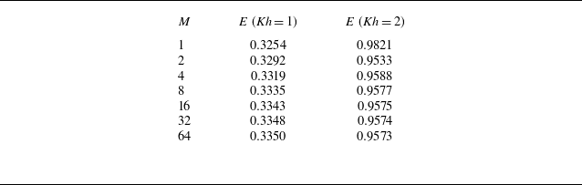
which controls the number of terms taken in the expansion of the approximate solution in (4.1). In table 1 we present a convergence example for a typical set of results in the middle of the resonant range of frequencies. We are reminded that the two values of
 $E=E_{\textit{ff}}$
and
 $E=E_{\textit{nf}}$
are numerically identical (apart from small rounding errors) and cannot be used to indicate accuracy of the method.
Computed values of efficiency,
 $E = E_{\textit{ff}} = E_{\textit{nf}}$
, for increasing truncation parameter,
 $M$
, for
 $\textit{Kh} = 1$
and
 $\textit{Kh}=2$
with
 $a/h = 0.1$
,
 $b/h = 0.4$
,
 $\tilde {\lambda }_1 = 5$
and
 $\tilde {\lambda }_2 = 0$
.

Table 1 Long description
A table comparing efficiency values for different truncation parameters. The table has 8 rows and 3 columns. The columns are labeled M, E (Kh = 1), and E (Kh = 2). The row labels are numerical values for M. The values in the columns are as follows: Row 1: M, 1, E (Kh = 1), 0.3254, E (Kh = 2), 0.9821. Row 2: M, 2, E (Kh = 1), 0.3292, E (Kh = 2), 0.9533. Row 3: M, 4, E (Kh = 1), 0.3319, E (Kh = 2), 0.9588. Row 4: M, 8, E (Kh = 1), 0.3335, E (Kh = 2), 0.9577. Row 5: M, 16, E (Kh = 1), 0.3343, E (Kh = 2), 0.9575. Row 6: M, 32, E (Kh = 1), 0.3348, E (Kh = 2), 0.9574. Row 7: M, 64, E (Kh = 1), 0.3350, E (Kh = 2), 0.9573.
Plots of the modulus of
 $\eta (x)$
against
 $x/h \in (0.1,0.4)$
for
 $a/h = 0.1$
,
 $b/h=0.4$
,
 $\tilde {\lambda }_1 = 5$
,
 $\tilde {\lambda }_2 = 0$
for four different values of
 $\textit{Kh}$
. Plots (a) and (b) are for
 $M=16$
and
 $M=32$
.

In figure 3(a,b) we show the computed value of
 $|\eta |$
, the modulus of the internal free surface amplitude non-dimensionalised by the incident wave height, as a function of
 $z \in (a,b)$
. For this, we use the relation
 $|\eta | = |1+R||u(z)|/K$
. Results are shown for truncation sizes of
 $M=16$
and
 $M=32$
for a fixed geometry and constant power control. The oscillations in the curves are explained by Gibbs phenomenon, but nevertheless demonstrate the convergence of approximations with increasing
 $M$
. In each figure curves represent different values of
 $\textit{Kh}$
to show how resonance is excited at positions (marked by the vertical dotted lines) along the duct dependent on frequency. For the device parameters chosen,
 $\textit{Kh} = 1$
is outside the resonant spectrum. We note that peak amplitudes are shifted slightly to the left of the position predicted using (6.1); figure 3(a,b) shows that, for the parameters chosen, device resonance corresponds to less than a doubling of the standing wave amplitudes that would occur if waves were reflected by a wall without the device in place. In figure 4 we have plotted real and imaginary parts of
 $\phi (x,z)$
across the fluid domain for some typical parameters which highlight the smooth matching of the potential across the duct opening. The colour scale is cropped to values between −3 and + 3, although
 $\textrm{Im} \{\phi (x,z)\}$
exceeds a value of 5 at the top of the duct. The two figures provide information about the significant variation in the phase of oscillations across the width of the duct resulting from resonance towards the centre.
The real and imaginary parts of
 $\phi$
for
 $a/h=0.25$
,
 $b/h=0.75$
,
 $\textit{Kh} = 1$
,
 $\tilde {\lambda }_1 = 5$
,
 $\tilde {\lambda }_2 = 0$
computed using
 $M=32$
.

6.3. The role of compressibility of air
The effect of compressibility in (4.9) is controlled by the size of the ratio of the imaginary and real parts of
 $\tilde {\varLambda }$
, or
 \begin{align} (\textit{Kh} (b/h - a/h))^{1/2} (\rho g H/\rho _a c_a^2)/\tilde {\lambda }_1 \approx 0.07 H \sqrt {\textit{Kh} (b/h-a/h)}/\tilde {\lambda }_1 \end{align}
(in SI units). For a full-scale installation we imagine
 $H$
to be roughly
 $4-5$
m and
 $(b/h - a/h)$
to be roughly
 $0.3-0.5$
whilst it seems reasonable to assume that
 $\textit{Kh} \lesssim 6$
is a range of practical interest (implying wavelengths no shorter than the water is deep). Then the maximum size of (6.3) is roughly
 $0.5/\tilde {\lambda }_1$
. So compressibility can become a significant factor if
 $\tilde {\lambda }_1$
is roughly one or less and for larger values of
 $\textit{Kh}$
. In terms of producing the optimal power output, it has been found that we should choose
 $\tilde {\lambda }_1 \approx 5$
, not only for results shown in figure 2 but also for other configurations tested. Then the size of the term in (6.3) never exceeds
 $0.1$
and we expect the effect of viscous damping on the efficiency to be proportionately small. These observations are bourne out in the results shown in figure 5(a).
In experiments one might imagine
 $H = 0.4-0.5$
m and then the size of the term in (6.3) is an order of magnitude smaller than in the full-scale setting meaning its effect is negligible, as shown in figure 5(b).
Variation of efficiency with
 $\textit{Kh}$
for
 $a/h=0.1$
,
 $b/h = 0.4$
. In (a)
 $\tilde {\lambda }_2 = 0.333$
and in (b)
 $\tilde {\lambda }_2 = 0.033$
;
 $\tilde {\lambda }_1$
is varied. The grey curves shadow the values computed in figure 2.

6.4. The role of viscosity
The size of
 $\tilde {\varGamma }$
defined by (5.4) in a full-scale installation is estimated to be of the order of
 $10^{-3}$
based, say, on 6 channels within a duct of the size
 $b-a = 3$
m. This is much smaller than the other
 $O(1)$
terms in (5.4). Even with many more channels, the influence of viscosity at full scale is going to be negligible. In experiments, we might imagine
 $b-a = 0.3$
m in which case
 $\tilde {\varGamma }$
is more like
 $10^{-2}$
and likely to still have only a small effect on results. Sample results are shown in figure 6(a).
Variation of device efficiency with
 $\textit{Kh}$
for
 $a/h=0.1$
,
 $b/h = 0.4$
. In (a)
 $\tilde {\lambda }_1 =5$
,
 $\tilde {\lambda }_2 = 0$
and different values of
 $\tilde {\varGamma }$
; in (b) spatially varying power control:
 $\alpha = 5$
and different values of
 $\tilde {\beta }$
.

6.5. Non-constant control parameters
We consider the effect of introducing spatial control of the damping by letting
 $\tilde {\lambda }_1(z) = \alpha \mathrm{e}^{-\beta z}$
, where
 $\alpha \gt 0$
and
 $\beta \neq 0$
are constants. For
 $\beta \gt 0$
the damping is weaker for the longer channels and vice versa whilst
 $\beta = 0$
corresponds to constant damping considered previously. Setting
 $\tilde {\lambda }_2 = 0$
allows us to explicitly calculate the terms required in the numerical scheme (see Appendix A). Figure 6(b) shows the results of fixing
 $\alpha = 5$
and varying
 $\tilde {\beta } = \beta /(b-a)$
between
 $-2$
and
 $2$
. Other combinations of
 $\alpha$
and
 $\tilde {\beta }$
have been considered but, as shown in figure 6(b), it seems that spatial control of damping does not result in significant improvements in the efficiency.
Comparision of efficiency with
 $\textit{Kh}$
for the current multi-chamber design and the single-chamber OWC of Evans & Porter (Reference Evans and Porter1995) in the cases that the front wall immersion is: (a)
 $0.25h$
; and (b)
 $0.1h$
.

6.6. Comparison with a simple single-chamber OWC
In figure 7 we have plotted a comparison of the performance, in terms of efficiency, of the current multi-channel (or multi-chamber) OWC design against the single-chamber OWC design of Evans & Porter (Reference Evans and Porter1995) for two cases. In the first case, the multi-chamber OWC parameters are
 $a = 0.25h$
and
 $b = 0.75h$
and this is compared with the Evans & Porter (Reference Evans and Porter1995) results with a barrier submergence of
 $0.25h$
and chamber width
 $0.75h$
. In the second example, we have chosen
 $a = 0.1h$
,
 $b=0.99h$
and results are compared with Evans & Porter (Reference Evans and Porter1995) with a barrier submergence of
 $0.1h$
and chamber width
 $h$
. In each case, air compressibility and viscous effects have been neglected and the value of the damping parameters for each curve produced have been chosen to ‘optimise’ the efficiency profile. The secondary narrow peak in figure 7(a) is the first in a sequence of peaks as frequency increases, associated with sloshing modes between the front and back walls of the single-chamber OWC. Thus, we can see that the multi-chamber OWC design does no better than a single-chamber design if immersion of the duct opening is too large. For a smaller immersion of the duct opening, the multi-chamber OWC outperforms the single-chamber OWC by a significant degree.
7. Conclusions
We have considered a two-dimensional model of a novel OWC concept which has been designed to exploit resonance over a broad range of frequencies. A simple mathematical model has been formulated by assuming regular waves of a single frequency under linearised theory and by approximating the complexity of the multi-channel duct using homogenisation. The general conclusion drawn from the various numerical experiments considered here is that the optimal configuration of an OWC, resulting in a high bandwidth, can be achieved by applying constant power control across the array of channels. It has been found that the effects of compressibility and viscosity may be neglected when applied to a full-scale installation, although these effects might influence test-scale experiments. The effects of viscosity have been modelled on an idealisation of the flow in the channels of the duct and is likely to have underestimated the dissipation occurring in real fluid flows.
From an engineering perspective a multi-chamber design is more complicated than a single-chamber OWC. The nature of the ocean energy density spectrum means that loads will be distributed across multiple generators in the array. As the device is designed to be fixed, tidal variation is an issue although the broadbanded response of the device allows it to function across a range of conditions. Moreover, the multi-channel design allows for a system of louvres, which shut different channels on and off to optimise performance in different sea conditions as well as being used for a complete shutdown of the device in storms. It should be noted that an alternative strategy would be to combine multiple channels to drive larger Wells turbines via a suitable packing configuration; however, this has not been investigated here.
Extensions to the current work might involve solving the problem of distinct channels within the duct exactly, without homogenisation. This might require the use of boundary element methods even for the two-dimensional problem because semi-analytic methods are not easy to apply to such geometries. It is possible to consider a three-dimensional version of this problem for a segmented OWC of finite width in an infinitely long wall using a combination of the methods described here and Fourier transforms. One would need to make a convincing case for adding extra complexity.
Funding
This research received no specific grant from any funding agency, commercial or not-for-profit sectors.
Declaration of interests
The authors report no conflict of interest.
Appendix A.
Below are the explicit definitions of the terms required in the numerical scheme. We define
 $c = (1/2) (a+b)$
and
 $d = (1/2) (b-a)$
. In the case that
 $r \neq 0$
we have
 \begin{align} F_{mr} = \frac {2 d (-1)^m \sin k_r d}{\big((k_r d)^2 - (m \pi )^2 \big)\cos k_r h} \left [ k_r d \cos k_r (h-c) + {\mathrm{i}} m \pi \sin k_r(h-c) \right ] \end{align}
and when
 $r=0$
this is
 \begin{align} F_{m0} = \frac {2 d (-1)^m \sinh k d}{\big((k d)^2 + (m \pi )^2 \big) \cosh kh} \left [ k d \cosh k (h-c) + {\mathrm{i}} m \pi \sinh k(h-c) \right ]. \end{align}
Next, we find that
 \begin{align} T_{qq} = 2 c d, \qquad \mbox{and} \qquad T_{qm} = \frac {2 d {\mathrm{i}} (-1)^{q+m}}{(q-m) \pi }, \quad (q \neq m). \end{align}
When
 $\tilde {\lambda }_1(z) = \alpha \mathrm{e}^{-\beta z}$
,
 $\tilde {\lambda }_2 = 0$
we have
 \begin{align} S_{qm} = \frac {2 d \mathrm{e}^{\beta c}}{\alpha } (-1)^{m+q} \frac { \sinh \beta d}{{\mathrm{i}} \pi (m-q) + \beta d}. \end{align}
 N

 Kh
 a/h=0.1
 b/h=0.4
 a/h=0.2
 b/h=0.8
 λ~2=0
 λ~1
 E=Eff=Enf
 M
 Kh=1
 Kh=2
 a/h=0.1
 b/h=0.4
 λ~1=5
 λ~2=0

 η(x)
 x/h∈(0.1,0.4)
 a/h=0.1
 b/h=0.4
 λ~1=5
 λ~2=0
 Kh
 M=16
 M=32

 ϕ
 a/h=0.25
 b/h=0.75
 Kh=1
 λ~1=5
 λ~2=0
 M=32

 Kh
 a/h=0.1
 b/h=0.4
 λ~2=0.333
 λ~2=0.033
 λ~1

 Kh
 a/h=0.1
 b/h=0.4
 λ~1=5
 λ~2=0
 Γ~
 α=5
 β~

 Kh
 0.25h
 0.1h

 Open access

