



Nomenclature
- WIG
-
wing-in-ground craft
- IAE
-
integrated absolute error
- AE
-
absolute error
- RT
-
rise time
- ST
-
settling time
- OS
-
overshoot
- ITAE
-
integrated time absolute error
- ISE
-
integrated squared error
- ITSE
-
integrated time squared error
- SSE
-
steady-state error
- PID
-
proportional-integral-derivative
-
 $m$
-
the total steps of the trajectory or the number of trajectory points
-
${h^{\rm{*}}}$
-
the target altitude
-
$c$
-
chord length of the wing
-
${t_r}$
-
the step where the WIG reached the target altitude
${h^{\rm{*}}}$
for the first time -
${h_t}$
-
altitude of the trajectory point in the
$t$
-th step -
${h_0}$
-
the initial altitude
-
$r_r^{\left( t \right)}$
-
the reward of RT for the
$t$
-th step -
$r_e^{\left( t \right)}$
-
the reward of AE for the
$t$
-th step -
${R_r}$
-
the cumulative rewards of RT for the trajectory
-
${R_e}$
-
the cumulative rewards of AE for the trajectory
-
$R$
-
the total reward evaluated for the trajectory
-
$R_r^{\left( t \right)}$
-
the RT reward for the trajectory whose RT=
$\,t\,$
-
$R_e^{\left( t \right)}$
-
the IAE reward for the trajectory whose RT=
$\,t\,$
-
$R_r^ \star $
-
the cumulative rewards of RT for the trajectory by the multi-objective method
-
$R_e^ \star $
-
the cumulative rewards of AE for the trajectory by the multi-objective method
-
${R^ \star }$
-
the total reward evaluated for the trajectory by the multi-objective method
-
$k$
-
the varying weight value for the RT part of the multi-objective function
-
$\alpha $
-
the varying weight for the original method to examine its invariance
-
${F^i}$
-
the inertial frame
-
${F^f}$
-
the WIG-fixed frame
-
${F^b}$
-
the body frame
-
${m_w}$
-
mass of the WIG
-
$F$
-
force on the WIG in the WIG-fixed frame
${F^f}$
-
$M$
-
moment on the WIG in the WIG-fixed frame
${F^f}$
-
$u$
-
velocity vector measured in the body frame
${F^b}$
-
$\dot u$
-
acceleration vector measured in the body frame
${F^b}$
-
${g^n}$
-
acceleration of gravity in the inertial frame
${F^i}$
-
$C_g^b$
-
transformation matrix from
${F^f}$
to
${F^b}$
-
$V$
-
velocity vector measured in the inertial frame
${F^i}$
-
$I$
-
moment of inertia


Greek symbol
-
$\lambda $
-
exponential base
-
$\omega $
-
angular velocity vector measured in the body frame
${F^b}$
-
$\dot \omega $
-
angular acceleration vector measured in the body frame
${F^b}$


1.0 Introduction
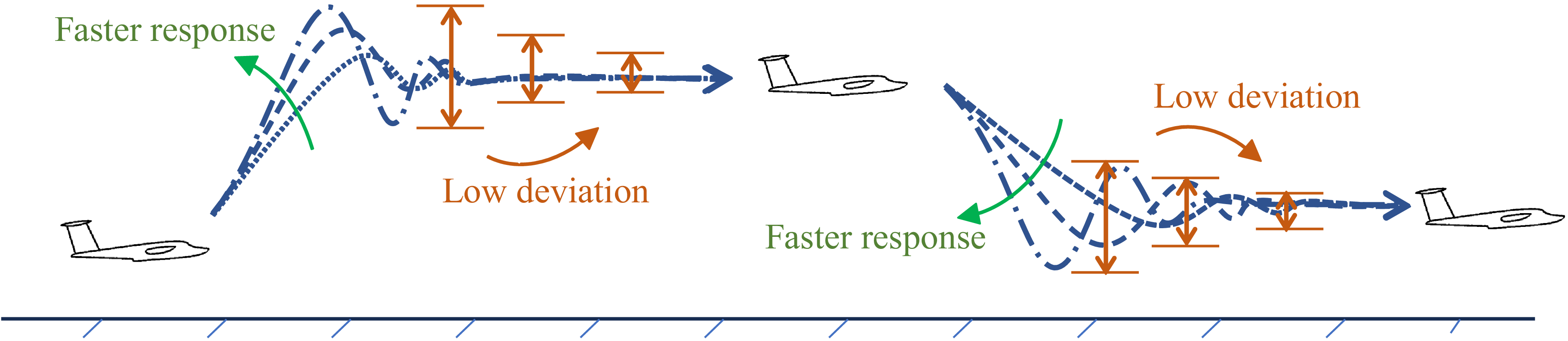
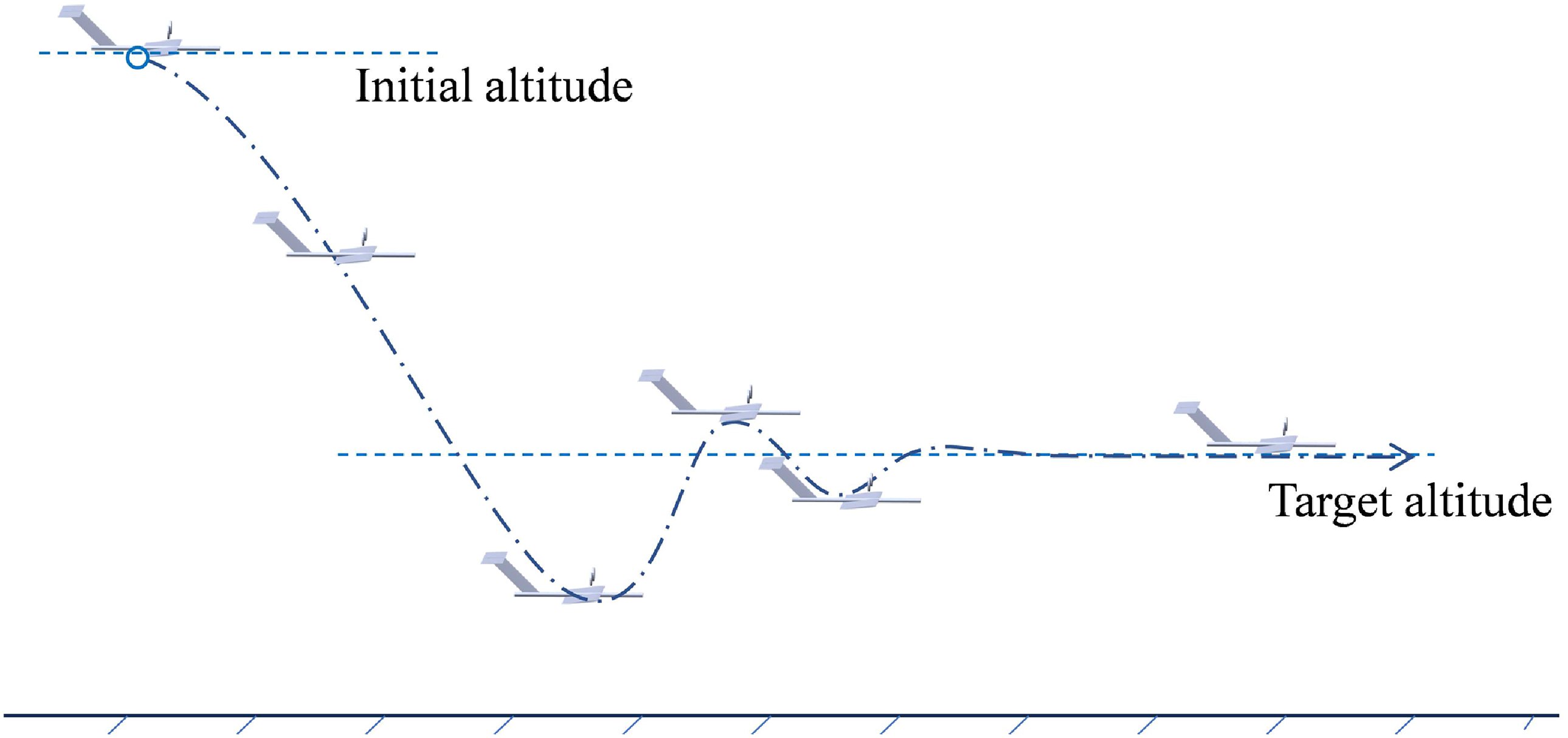
As a transitional vehicle between hovercraft and seaplanes, wing-in-ground (WIG) crafts typically maintain low flight altitudes to utilise ground effect, which provides a high lift-to-drag ratio and enhanced payload capacity. This operational mode also offers the militarily valued advantage of low observability. When encountering obstacles, waves or mission-specific requirements, WIG crafts must adjust their altitude. The ability to rapidly reach a target altitude and maintain minimal deviation during subsequent stabilisation demonstrates superior control performance. This manoeuvre is illustrated in Fig. 1.
The manoeuvring of a WIG is similar to that of an aircraft, so its motion response is a typical second-order model. Regarding trajectory planning for flight altitude adjustments, the absolute error (AE) is commonly adopted as the basis for reward functions. AE quantifies the minimum distance between the current position and the target trajectory or altitude. By integrating the AE across multiple trajectory points, the integrated absolute error (IAE) is obtained, which serves as a metric for evaluating the overall deviation between the current and target trajectories. In studies on nonlinear control strategies [Reference Patria, Rossi, Fernandez and Dominguez1], nonlinear adaptive control systems [Reference Panferov, Nebylov and Brodsky2] and feedback control [Reference Daniel3] for switching the WIG’s flight altitude, there are distinctive second-order motion responses, with different performance of rise time (RT), settling time (ST) and overshoot (OS). There are also some studies on motion planning, where the reward function is designed with the help of integrated absolute error (IAE) to realise the WIG’s trajectory planning, such as reducing the OS [Reference Hu, Zhang, Ding, Jiao, Zhang and Zhang4], stabilising the landing control [Reference Zhang, Hu, Zhang, Zhang and Wang5, Reference Zhang, Hu, Zhang and Zhang6] or meeting multiple kinds of flight requirements [Reference Hu, Li, Zhang and Zhang7]. However, taking a closer look at these studies, it can be found that minimising IAE cannot guarantee whether the WIG adjusts its altitude quickly enough. If the change of WIG’s altitude is rapid, the WIG will reach the target altitude earlier; in other words, RT of the trajectory will be smaller. Then, the extent to which the WIG’s flight exceeds the target altitude will be greater due to its inertia, leading to a larger OS. Next motion is that the WIG oscillates up and down and gradually approaches the target altitude. This process of convergence will be longer, resulting in a greater ST of the trajectory. Generally, IAE will be greater for a more zigzag trajectory. It can be seen that there is a contradictory relationship between RT and full-trajectory IAE.
Studies in recent years have incorporated various metrics, including IAE, RT and ST, as partial terms in trajectory adjustment. These terms are typically incorporated linearly into the reward function as penalty terms, with coefficients or exponents used to adjust the trajectory towards desired behaviours. For wind energy maximum power point tracking (MPPT), multi-objective genetic algorithms (GA) simultaneously minimised integrated time absolute error (ITAE), integrated squared error (ISE), IAE and integrated time squared error (ITSE) [Reference Mrabet, Benzazah, El Akkary, Ennaciri and Lahlouh8], while GA and ant colony optimisation were also employed to minimise ITAE [Reference Mrabet, Benzazah, Mohssine, Ahmed, Driss, Badr and Ilyas9, Reference Mrabet, Benzazah, El Akkary, Chakib and Lahlouh10]. ITAE weights AE by time
 $t$
. Formally, it assigns a weight of
 $t$
to the AE at each time step. In essence, it treats AEs at different time steps as distinct objectives to be coordinated, with the importance of subsequent AEs increasing progressively with the elapsed time. This is equivalent to formulating a multi-objective function. In load frequency control, sunflower optimisation, teaching–learning-based optimisation and GA were compared with ITAE as the cost [Reference Nayak, Nayak, Prusty and Panda11], and particle swarm optimisation (PSO)-tuned fuzzy controllers were evaluated via ISE, IAE, mean squared error (MSE) and ITAE [Reference Nasir, Ghani, Nasir, Ahmad and Tokhi12]. To more explicitly balance transient specifications, many authors constructed composite objective functions. Ghosh et al. [Reference Ghosh, Ray, Nurujjaman and Jamshidi13] built an objective combining ISE, OS and ST, via PSO; Samuk and Çakr [Reference Samuk and Çakr14] employed radial movement optimisation with a multi-variable objective that combined classical error integrals (ITAE, ISE, IAE, ITSE) with transient parameters (maximum OS and ST) using weight coefficients. Cárdenas et al. [Reference Cárdenas, Carrero, Camacho and Calderón15] compared four multi-objective PSO cost functions merging ST, OS and steady-state error (SSE). Weighted sums of IAE, ISE and ITAE were minimised via enhanced GA [Reference Kushary and Barai16], while animated oat optimisation and PSO used IAE, ISE, ITAE and ITSE for inverter control [Reference Thampi and Mahendran17]. Multi-objective PSO also simultaneously reduced ST and torque ripple [Reference Shashibhushan and Sonoli18]. Further works explicitly integrated OS, ST and RT into the fitness function for multi-objective GA [Reference Cojuhari, Fiodorov, Izvoreanu and Moraru19], or modified classical error integrals by adding weighted ST, RT, OS percentage and SSE [Reference Zahir, Alhady, Wahab and Ahmad20], by the method of GA. Time-domain objective functions aggregating maximum OS, SSE, RT and ST have been optimised by opposition-based hybrid manta ray foraging and simulated annealing [Reference Ekinci, Izci and Hekimoğlu21], by PSO [Reference Rahayu, Ma’arif and Cakan22] and by an opposition-based weighted mean of vectors algorithm [Reference Ekinci, Can and Izci23]. The Zwee-Lee Gaing (ZLG) function, which combines SSE, OS, ST and RT, was employed with the artificial rabbits optimiser [Reference Abualigah, Izci, Ekinci and Zitar24] and with the equilibrium optimiser [Reference Micev, alasan and Oliva25]. A custom fitness function comprising OS, RT, ST and steady-state error was designed for PSO and differential evolution [Reference Can and Ercan26]. PSO combined with gravitational search algorithm optimised fall time, symmetrical rise/fall times and propagation delays [Reference Fantin and Mohanbabu27], and the rime optimisation algorithm tuned a delay-affected controller using a composite objective integrating IAE, ITAE, ISE, SSE, RT, ST and OS [Reference Yüksek28].
The WIG’s fast-response and low-deviation trajectory during altitude transition.

A similar weighted objective philosophy appears in reinforcement learning, where reward functions are designed as weighted sums of multiple terms to provide step-by-step feedback for learning an adaptive policy. Deep deterministic policy gradient (DDPG) has been applied to missile control with a reward comprising minimum error (effectively IAE), excessive error and excessive deflection rate [Reference Taligatos, Nguyen and Lowenberg29]. For an optoelectronic stabilisation platform, DDPG combined with a fractional-order proportional-integral-derivative (PID) controller used a reward considering accuracy (IAE-related), stability, response speed and energy consumption [Reference Zhao, Sun, Shi and Tiwari30]. A comparative study of proximal policy optimisation (PPO), DDPG, advantage actor-critic (A2C) and twin-delayed deep deterministic policy gradient (TD3) for spacecraft attitude recovery designed an exponential signal reward with an accuracy term corresponding to an IAE-like measure and a rate penalty [Reference Ahmadi, Mirji, Peng, Luo and Ahmadi31]. In reinforcement learning-based model predictive control, TD3 was embedded with a cost function whose first term stabilises stator currents (IAE minimisation) and second term penalises control increments [Reference Delelew, Dulecha, Ararso and Abdissa32]. TD3 was also used to tune cascaded proportional-integral (PI) controllers for a five-phase motor drive, with the reward implicitly minimising speed and torque errors, which essentially correspond to an IAE metric [Reference Hassan, Ababneh, Attar, Shamseldin, Abdelbaset and Metwally33].
However, prior research lacks specific guidance on how to determine appropriate values for these coefficients or exponents. While most studies qualitatively analyse how these penalty terms influence the trajectory, there has been limited quantitative assessment of their effect. As a result, no precise method exists for determining the optimal coefficient or exponent values. In conventional approaches, metrics such as RT and IAE are combined into a multi-objective reward, with each term assigned an individual weight. The relative magnitudes of these weights are typically adjusted through trial and error to align the trajectory with the desired outcome. This process aims to reduce IAE or RT, ultimately bringing the trajectory closer to the target altitude or allowing the WIG to reach the target altitude more quickly. However, this method lacks precision and requires iterative adjustments. For trajectory planning, especially in obstacle scenarios, the goal is to minimise RT first and then approach the target altitude as closely as possible. Designing a reward function that directly achieves this priority remains a significant engineering challenge.
The innovation of this paper is to propose a reward function for trajectory planning, which satisfies the preferential minimisation of RT and subsequent minimisation of IAE. The engineering contribution is directly guiding the WIG to change its altitude as quickly as possible, and then approach the target altitude as fast as possible. When evaluating a trajectory where there are remaining
 $n$
steps after the WIG reaches the target altitude, the IAE-related part of the reward function evaluates IAE for the last
 $n$
steps, while the RT-related part is assigned based on the maximum value of IAE. If the RT can be reduced by one step, in other words, if the WIG reach the target altitude one step ahead, the RT-related reward will increase the maximum value of IAE, so as to drive the WIG to the target altitude in advance. In this way, the RT-related item can be expressed as a triangular number, i.e.
 $n$
*(
 $n$
+1)/2, and the feasibility of the method is demonstrated by mathematical reasoning.
In the following sections, the construction of the proposed reward function is demonstrated; then the model and optimisation methods which are used for its validation are introduced. Next, based on the results obtained by the proposed reward function and the conventional multi-objective reward function, comparison and further analysis are conducted. Finally, the conclusion is drawn.
2.0 Reward function
2.1 Form
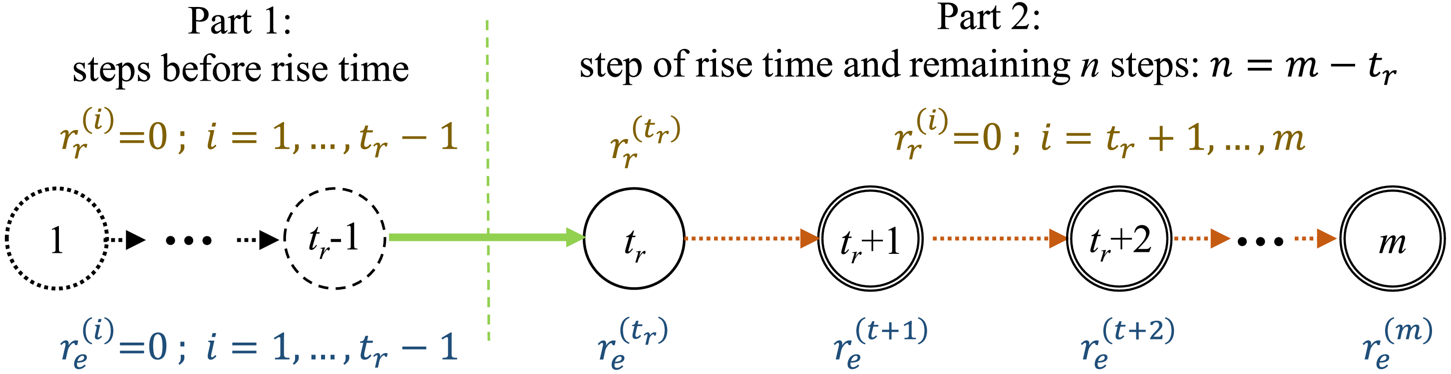
Assume that the WIG traverses a trajectory consisting of
 $m$
steps and has not reached the target altitude
 ${h^{\rm{*}}}$
by the
 ${t_r}$
-th step. The whole trajectory can be divided into two parts by the step
 ${t_r}$
, as illustrated in Fig. 2. To evaluate an optional trajectory, two kinds of reward are calculated in each step, which are named as
 $r_r^{\left( t \right)}$
representing the reward of RT and
 $r_e^{\left( t \right)}$
representing the reward of AE, expressed as:
 \begin{align} r_e^{\left( t \right)} = \left\{ {\begin{array}{*{20}{l}}{0,} \quad \qquad\qquad\qquad{{\rm{if\;}}t \lt {t_r}}\\[6pt]{1 - \left| {\dfrac{{{h_i} - {h^{\rm{*}}}}}{{{h^{\rm{*}}} - {h_0}}}} \right|,} {} \quad \quad{{\rm{if\;}}t \geqslant {t_r}}\end{array}} \right. \end{align}
 \begin{align}r_r^{\left( t \right)} = \left\{ {\begin{array}{*{20}{l}}{0,} \qquad \quad \quad \ \qquad\quad\qquad \qquad {{\rm{if\;}}t \ne {t_r}}\\[6pt]{1 + \dfrac{{n\,{\rm{*}}\left( {n + 1} \right)}}{2}{\rm{\;}},{\rm{\;\;}}n = m - t,} \quad {{\rm{if\;}}t = {t_{}}}\end{array}} \right. \\[3pt] \nonumber \end{align}
where
 ${h_i}$
is the WIG’s flight altitude at the
 $i$
-th step.
 ${h_0}$
is the initial altitude at the beginning of the trajectory, where the WIG starts to operate.
 $n$
is the number of remaining steps after RT occurs, i.e., steps (
 $t$
+1) to
 $m$
, so
 $n = m - t$
. For the whole trajectory, these two kinds of corresponding cumulative rewards are
 ${R_r}$
and
 ${R_e}$
, respectively, and their sum is the reward evaluated for the trajectory, given as:
 \begin{align} {{R_r} = \mathop \sum \limits_{t = 1}^m r_r^{\left( t \right)}} \nonumber \\[3pt] {{R_e} = \mathop \sum \limits_{t = 1}^m r_e^{\left( t \right)}} \\[3pt] {R = {R_e} + {R_t}} \nonumber \end{align}
The division of the whole trajectory and reward for different steps.

Rewards for parts of a trajectory are also shown in Fig. 2.
 $r_e^{\left( t \right)}$
are assigned as 0 for steps from the first to the (
 ${t_r}$
-1)-th, where RT has not occurred. With the exception of the
 ${t_r}$
-th step,
 $r_t^{\left( t \right)}$
of all other steps are set to 0.
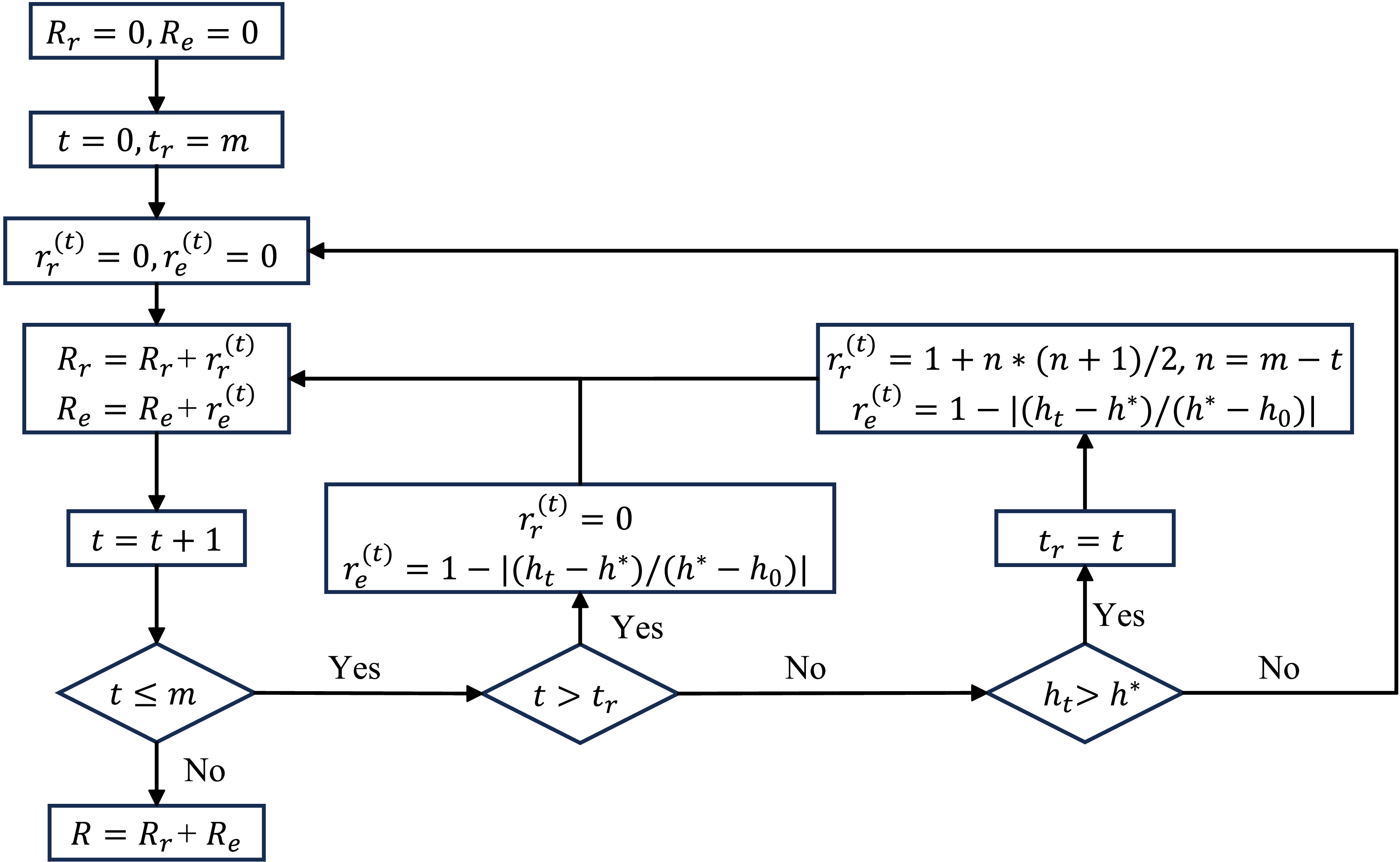
The process by which the reward function assesses the reward of an available trajectory where the WIG adjusts its altitude to a higher one is as follows, and the algorithm operates as 9(‘)@, whose flowchart is shown in Fig. 3. It proceeds in the forward direction from the initial state to the end of the trajectory, with the RT initially assumed to occur at the final step, i.e.
 $m$
-th step. When the WIG’s flight altitude exceeds the target altitude for the first time at an intermediate step, the occurrence of the RT is identified, and the corresponding
 ${t_r}$
for that trajectory is thereby determined. In the current study, which considers the case of the WIG reducing its flight altitude, the condition
 $h\,{\rm{*}} \gt {h_t}$
is used to determine whether the RT has occurred.
-
(1) Give the trajectory with the altitude of each trajectory point
${h_t}$
,
$t\,$
=
$\,1,2 \ldots m$
. -
(2) Initially, the order of the current step,
$t$
=1. Initially, the total RT-related and total IAE-related reward,
${R_r}\,$
= 0 and
${R_e}\,$
= 0. -
(3) Assume the rise time occurs at the last step, as
${t_r}\,$
=
$\,m$
. -
(4) If the current step
$t$
is after
${t_r}$
, meaning that
$t \gt {t_r}$
, the current step RT reward
$r_r^{\left( t \right)}$
is assigned 0, and the current step AE reward
$r_e^{\left( t \right)}$
is calculated by Equation (1) based on the current flight altitude
${h_t}$
. -
(5) If
$t \lt {t_r}$
and
${h_t}$
is higher than the target altitude
${h^{\rm{*}}}$
,
${t_r}$
is replaced by
$t$
.
$r_r^{\left( t \right)}$
and
$r_e^{\left( t \right)}$
are calculated by Equations (1) and (2), respectively. -
(6) If
$t \lt {t_r}$
and
${h_t} \lt {h^{\rm{*}}}$
,
$r_r^{\left( t \right)}$
and
$r_e^{\left( t \right)}$
are both assigned 0. -
(7) Accumulate
$r_r^{\left( t \right)}$
and
$r_e^{\left( t \right)}$
to the total RT-related reward
${R_r}$
and total IAE-related reward
${R_e},$
respectively. -
(8) Proceed one step forward, and loop through steps (4) to (7), until the current step reaches the end.
-
(9) Summarise
${R_r}$
and
${R_e}$
as the total reward
$R$
of the trajectory.


Workflow of reward evaluation on the trajectory.

2.2 Proof
Assuming there are multiple trajectories for the WIG to manoeuvre during altitude change, consider one trajectory
 $T$
with RT as
 ${t_r}$
. For comparison, there exists another trajectory
 $T{\rm{'}}$
with a smaller RT denoted as
 ${t'_{r}}$
, assuming
 ${t'_{r}} = {t_r} - \delta $
. The respective rewards for the two trajectories are labeled as
 $R$
and
 $R{\rm{'}}$
, which can be combined using Equations (1), (2) and (3), then expressed as:
 \begin{align} R = \mathop \sum \limits_{t = {t_r}}^m r_e^{\left( t \right)} + {{n\,{\rm{*}}\left( {n + 1} \right)} \over 2} + 1{\rm{\;}},{\rm{\;}}n = m - t \\[-10pt] \nonumber \end{align}
 \begin{align} R{\rm{'}} = \mathop \sum \limits_{t = {t'_{r}}}^m {r'_{e}}^{\left( t \right)} + {{n{\rm{'*}}\left( {n{\rm{'}} + 1} \right)} \over 2} + 1{\rm{\;}},{\rm{\;}}n{\rm{'}} = m - t' \\[10pt] \nonumber \end{align}
where
 ${r'_{e}}^{\left( t \right)}$
and
 $n{\rm{'}}$
are the AE reward of each step and the number of subsequent steps after RT for
 $T{\rm{'}}$
,
 $n{\rm{'}} = n + \delta $
.
 $R{\rm{'}}$
minus
 $R$
gives:
 \begin{align}{\rm{\Delta }}R = R{\rm{'}} - R = \mathop \sum \limits_{t = {t'_{r}}}^m {r'_{e}}^{\left( t \right)} - \mathop \sum \limits_{t = {t_r}}^m r_e^{\left( t \right)} + \delta \,{\rm{*}}\left(n + {{\delta + 1} \over 2}\right)\\[-25pt] \nonumber \end{align}
Algorithm 1

Algorithm 1 Long description
The algorithm starts by inputting the altitude of each trajectory point. It initializes variables R subscript r and R subscript e to 0, and t to 0. The time step of rise time is assumed as t subscript r equals m. A while loop runs as long as t is less than or equal to m. Inside the loop, if t is greater than t subscript r, r subscript r superscript t and r subscript e superscript t are set to 0 and 1 minus the absolute value of h subscript t minus h asterisk divided by h asterisk minus h subscript 0, respectively. If h subscript t is greater than h asterisk, t subscript r is set to t, r subscript r superscript t is set to 1 plus n times n plus 1 divided by 2, where n equals m minus t, and r subscript e superscript t is set to 1 minus the absolute value of h subscript t minus h asterisk divided by h asterisk minus h subscript 0. If neither condition is met, r subscript r superscript t and r subscript e superscript t are set to 0. R subscript r and R subscript e are updated by adding r subscript r superscript t and r subscript e superscript t, respectively, and t is incremented by 1. The loop continues until t exceeds m. Finally, R is calculated as the sum of R subscript r and R subscript e, and R is outputted.
To explore the minimum value of
 ${\rm{\Delta }}R$
, note that the per-step AE reward lies within [0,1] for
 $r_e^{\left( t \right)}$
and
 ${r'_{e}}^{\left( t \right)}$
. Since
 $\mathop \sum \nolimits_{t = {t'_{r}}}^m {r'_{e}}^{\left( t \right)}$
appears as an additive term, its minimum value should be taken as 0. In contrast,
 $\mathop \sum \nolimits_{t = {t_r}}^m r_e^{\left( t \right)}$
appears as a subtractive term, and thus its maximum,
 $n + 1$
, should be used. Consequently,
 ${\rm{\Delta }}R$
can be derived as:
 \begin{align}{\rm{\Delta }}R = \delta\, {\rm{*}}\left( {n + \frac{{\delta + 1}}{2}} \right) - \left( {n + 1} \right) \\[-30pt] \nonumber \end{align}
Given that
 $\delta $
is a positive integer,
 $\delta \geqslant 1$
, the value of
 ${\rm{\Delta }}R$
is therefore never less than 0,
 ${\rm{\Delta }}R \geqslant 0$
. Moreover, since the boundary value cannot be reached in practice,
 ${\rm{\Delta }}R$
is greater than 0,
 ${\rm{\Delta }}R \gt 0$
. As the optimisation algorithm seeks trajectories with larger reward, it will prefer
 $T{\rm{'}}$
over due to its higher reward, thereby driving RT to decrease, as:
 \begin{align}R \lt R{\rm{'}} \Rightarrow T \to T' \Rightarrow {t_r} \to {t'_{r}} \end{align}
Meanwhile, the smaller the deviation, the larger the IAE reward becomes.
2.3 Interpretation
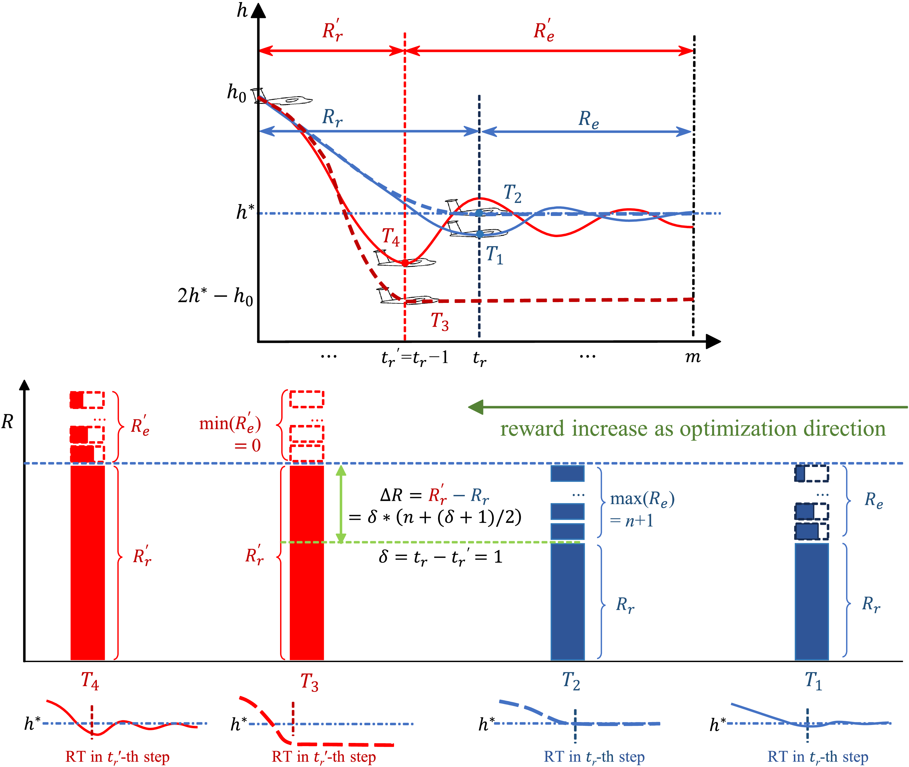
For comparison, trajectories where RT occurs in the
 ${t_r}$
-th and
 ${t'_{r}}$
-th step is selected, assuming
 ${t'_{r}}$
=
 ${t_r}$
-1. Figure 4 illustrates both typical and extreme cases for these two types of trajectories.
 ${T_1}$
represents a typical possible trajectory. After RT, if there is some deviation from the target altitude that does not reach the maximum, the reward
 ${R_e}$
will not be maximised. If no deviation from the target altitude occurs after RT, as in trajectory
 ${T_2}$
,
 ${R_e}$
reaches its maximum value, and this trajectory achieves the highest possible reward for RT=
 $t$
. When RT decreases, if the deviation after RT reaches its maximum, as in trajectory
 ${T_3}$
, the reward
 ${R_{e{\rm{'}}}}$
drops to its minimum of zero, representing the lowest possible reward for RT=
 $t{\rm{'}}$
. A more common case with sub-maximum deviation is trajectory
 ${T_4}$
, where
 ${R_{e{\rm{'}}}}$
is greater than zero. To drive the transition from trajectories with RT=
 ${t_r}$
to those with RT=
 $t{{\rm{'}}_r}$
feasibly through reward shaping, it must be ensured that the lower bound of the reward evaluation for RT=
 $t{{\rm{'}}_r}$
trajectories is no less than the reward value for RT=
 ${t_r}$
trajectories. Therefore, the following equation must be satisfied:
 \begin{align}{R_{r{\rm{'}}}} = {R_r} + {\rm{max}}\,\left( {{R_e}} \right) \end{align}
The comparison of the reward for trajectories whose RT occurs at
 $t$
-th step and (
 $t{\rm{'}}$
)-th step, respectively.

The RT reward after a one-step reduction must equal the sum of the RT reward and the maximum achievable IAE reward before the reduction. This condition enables the transition from trajectory
 ${T_2}$
to
 ${T_3}$
and makes it possible to drive the reduction in RT. This relationship can be formally expressed as
 \begin{align}{R_{r{\rm{'}}}} - {R_r} \geqslant {R_e} \end{align}
Physically, this equation implies that the incremental gain in RT reward resulting from a one-step decrease in RT should be greater than the loss of IAE reward caused by the RT reduction. In more general cases, such as trajectories
 ${T_1}$
and
 ${T_4}$
, the RT reward gain exceeds the corresponding IAE loss. Moreover, the trajectory after RT reduction still retains a residual IAE reward. These effects collectively promote the transition from trajectories like
 ${T_1}$
toward those like
 ${T_4}$
.
The above reasoning applies to adjacent RT differing by exactly one time step. This concept can be generalised to multi-step RT differences through iterative computation, allowing derivation of the RT reward for RT occurring at any arbitrary step. For notational clarity,
 $R_r^{\left( t \right)}$
and
 $R_e^{\left( t \right)}$
represent the RT reward and IAE reward, respectively, when RT=
 $t$
, that can be derived step-by-step backwards, as:
 \begin{equation}\begin{aligned}{R_r^{\left( t \right)}} {}& { = R_r^{\left( {t + 1} \right)} + {\rm{max}}\left( {R_e^{\left( {t + 1} \right)}} \right)}\\[5pt]{} {}& { = R_r^{\left( {t + 2} \right)} + {\rm{max}}\left( {R_e^{\left( {t + 2} \right)}} \right) + {\rm{max}}\left( {R_e^{\left( {t + 1} \right)}} \right)}\\[5pt]{} {}& {\qquad\qquad\qquad \vdots }\\[5pt]{} {}& { = R_r^{\left( m \right)} + {\rm{max}}\left( {R_e^{\left( m \right)}} \right) + {\rm{max}}\left( {R_e^{\left( {m - 1} \right)}} \right) \cdots + {\rm{max}}\left( {R_e^{\left( {t + 2} \right)}} \right) + {\rm{max}}\left( {R_e^{\left( {t + 1} \right)}} \right)}\\[5pt]{} {}& { = R_r^{\left( m \right)} + 1 + 2 + 3 + \cdots + n}\\[5pt]{} {}& { = 1 + \dfrac{{n\left( {n + 1} \right)}}{2}}\end{aligned} \end{equation}
where
 $R_r^{\left( m \right)}$
is defined as the initial RT reward for the situation where RT occurs at the last step,
 $m$
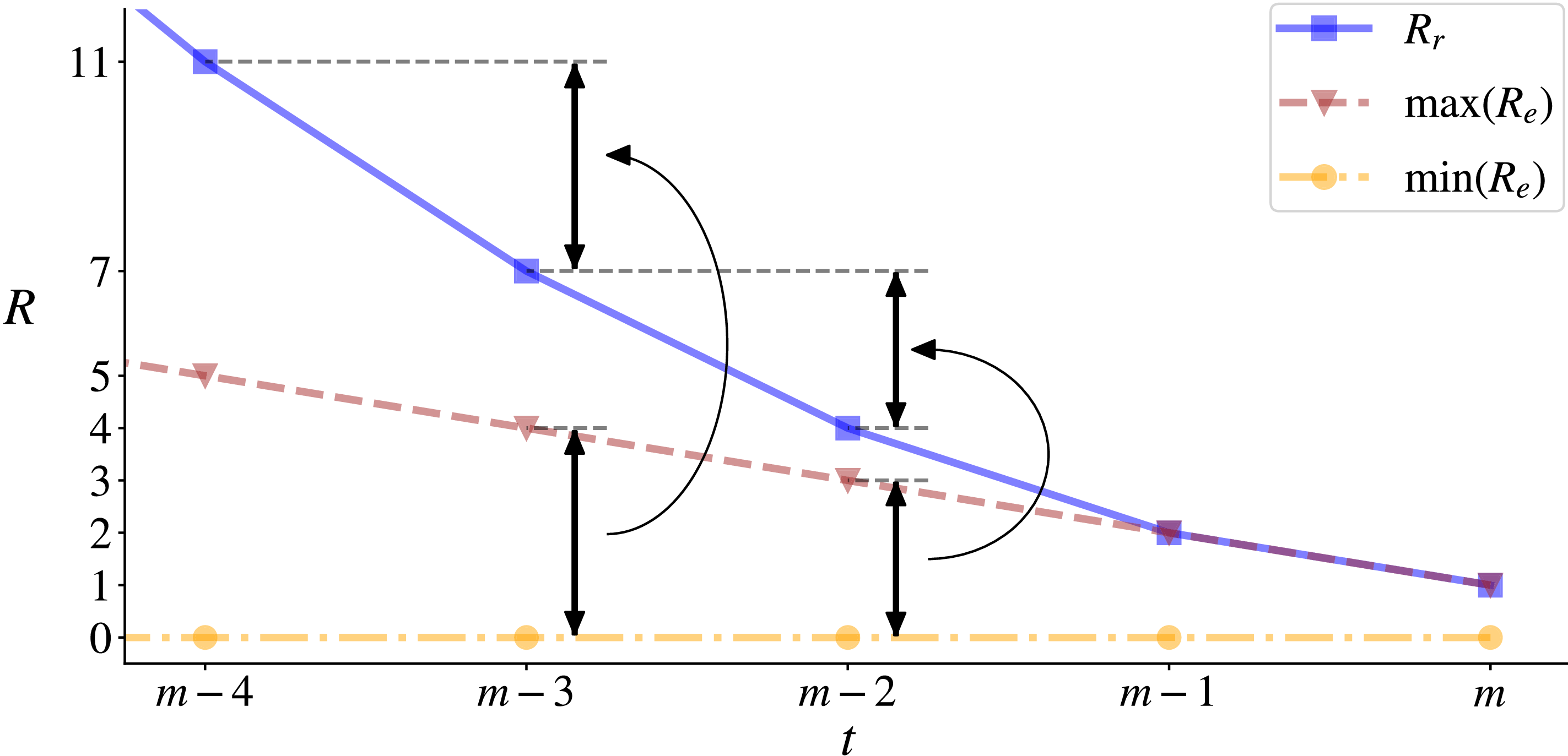
-th step. To prioritise achieving RT in the final step of the trajectory, the RT reward value should not exceed the maximum AE, i.e. 1. From the end to the beginning, the reverse analysis of RT reward for the step where RT happens is conducted to define its magnitude, illustrated in Fig. 5.
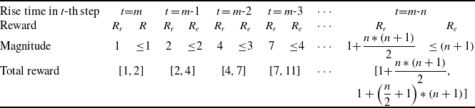
Table 1 shows the upper and lower bounds of the reward for trajectories whose RT occurs at different steps. Moving from left to right, the RT becomes progressively smaller. Although
 ${R_r}$
and
 ${R_e}$
is greater and greater, the maximum of the total reward is the same as the minimum of that when RT occurs in one earlier step. The staircase-like pattern strictly drives the trajectory to shift towards the direction of RT’s decrease.
Bounds of reward for the trajectory whose rise time occurs in different steps

Table 1. Long description
The table is labeled as Table 1 and titled Bounds of reward for the trajectory whose rise time occurs in different steps. It shows the relationship between rise time in different steps and the corresponding reward magnitude and total reward. The table has two columns: Rise time in -th step and Reward Magnitude. The rise time steps are labeled as equals, equals minus 1, equals minus 2, and equals minus 3. The reward magnitude values are 1, 1, 2, 2, 4, 3, 7, and 4. The total reward is given as 1 plus, open parenthesis 1 plus n times open parenthesis n plus 1 close parenthesis divided by 2 close parenthesis.
RT reward
 ${R_r}$
and the bounds of IAE reward
 ${R_e}$
if rise time occurs in the last five steps.

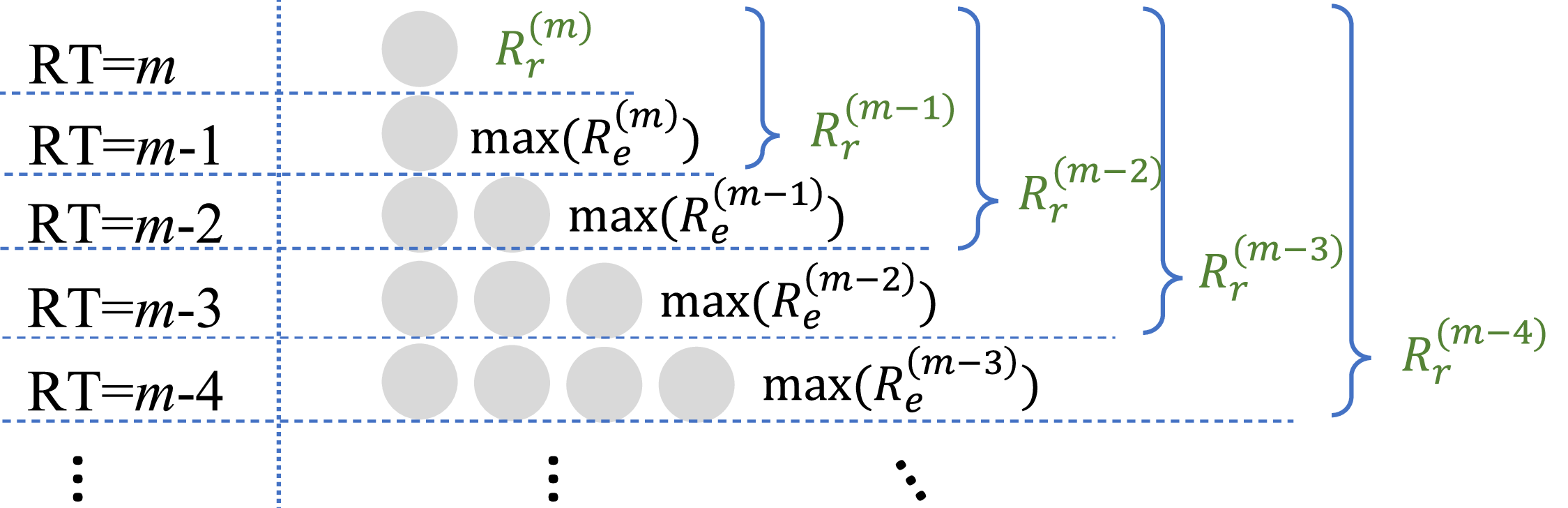
The RT reward value exhibits a form similar to the sum of an arithmetic sequence, i.e.
 $n$
*(
 $n$
+1)/2 concerning the remaining steps, which is the triangular number shown in Fig. 6.
The form of a triangular number for the construction of the RT reward
 ${R_r}$
based on IAE reward
 ${R_e}$
.

3.0 Simulation and method
3.1 Flight simulation
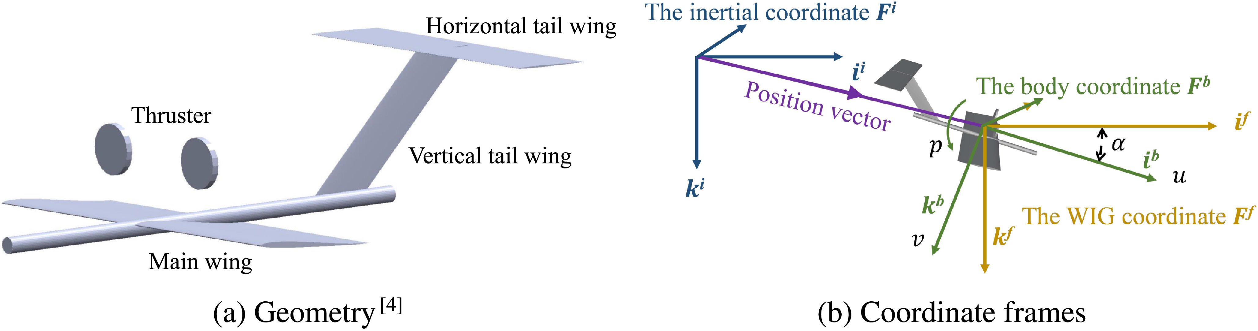
Validation is carried out using a dynamic and kinematic model of a small WIG operating in the longitudinal plane. The model has three degrees of freedom, with control surfaces consisting of an elevator and a propulsion [Reference Hu, Zhang, Ding, Jiao, Zhang and Zhang4]. Its geometrical shape and coordinate frames are shown in Fig. 7. The inertial frame
 ${F^i}$
is a fixed Earth-based reference frame, with its origin located at a specified home position. Its unit vector
 ${i^i}$
points forward, and
 ${k^i}$
points downward. The WIG-fixed frame
 ${F^f}$
is attached to the vehicle’s centre of gravity (
 $CG$
), and its axes are aligned with those of the inertial frame. The body frame
 ${F^b}$
also originates at
 $CG$
, but its axes move with the vehicle:
 ${i^b}$
points toward the nose, and
 ${k^b}$
points downward along the belly direction [Reference Beard and McLain34]. The WIG’s state quantities are displacements and angles along with their first and second derivatives, and the flight altitude can be extracted from the state. Aerodynamic forces applied to the WIG are computed using the vortex lattice method and image method [Reference Hu, Zhang, Ding, Jiao, Zhang and Zhang4], and then fed into the kinematic model to calculate the WIG’s motion response.
 \begin{align} \dot {\boldsymbol{u}} = {\boldsymbol{u}} \times {\omega} + {\boldsymbol{C}}_{\boldsymbol{g}}^{\boldsymbol{b}} \cdot \left( {\frac{{\boldsymbol{F}}}{{{m_w}}} + {\boldsymbol{g}}^{\boldsymbol{n}}} \right) \\[-10pt] \nonumber \end{align}
 \begin{align} \dot \omega = {{\boldsymbol{I}}^{ - 1}}\left( { - \omega \times {\boldsymbol{I}}\omega + {\boldsymbol{M}}} \right) \\[10pt] \nonumber\end{align}
where
 ${m_w}$
is mass of the WIG.
 $\boldsymbol{u} = {\left[ {u,0,w} \right]^T}$
and
 $\omega = {\left[ {0,q,0} \right]^T}$
denote the translational and angular velocity vectors in the body frame
 ${F^b}$
. The aerodynamic force and moment vectors are given by
 $\boldsymbol{F} = {\left[ {{F_x},0,{F_z}} \right]^T}$
and
 $\boldsymbol{M} = {\left[ {0,{M_y},0} \right]^T}$
, respectively. Gravity in the inertial frame is represented as
 ${\boldsymbol{g}^\boldsymbol{n}} = {\left[ {0,0,g} \right]^T}$
, and
 $m$
is the vehicle mass. Velocities
 $u$
and
 $w$
are along the body axes
 ${i^b}$
and
 ${k^b}$
, with their derivatives
 $\dot u$
and
 $\dot w$
indicating linear accelerations. The pitch rate
 $q$
is the angular velocity about
 ${j^b}$
. Forces
 ${F_x}$
and
 ${F_z}$
act along
 ${i^f}$
and
 ${k^f}$
in the WIG-fixed frame
 ${F^f}$
, while
 $g$
denotes gravitational acceleration. The transformation matrix
 $\boldsymbol{C}_\boldsymbol{g}^\boldsymbol{b}$
converts vectors from
 ${F^f}$
to
 ${F^b}$
. The inertial velocity
 $\boldsymbol{V} = {\left[ {{V_x},0,{V_z}} \right]^T}$
is obtained via
 $\boldsymbol{V} = \boldsymbol{C}_\boldsymbol{b}^\boldsymbol{g} \cdot \boldsymbol{u}$
, where
 ${V_x}$
and
 ${V_z}$
are velocity components along
 ${i^i}$
and
 ${k^i}$
, and
 $\boldsymbol{C}_\boldsymbol{b}^\boldsymbol{g} = {\left( {\boldsymbol{C}_\boldsymbol{g}^\boldsymbol{b}} \right)^T}$
. The inertia tensor is denoted by
 $\boldsymbol{I}$
.
The WIG’s geometry and coordinate frames for describing the WIG’s motion.

3.2 Optimisation method
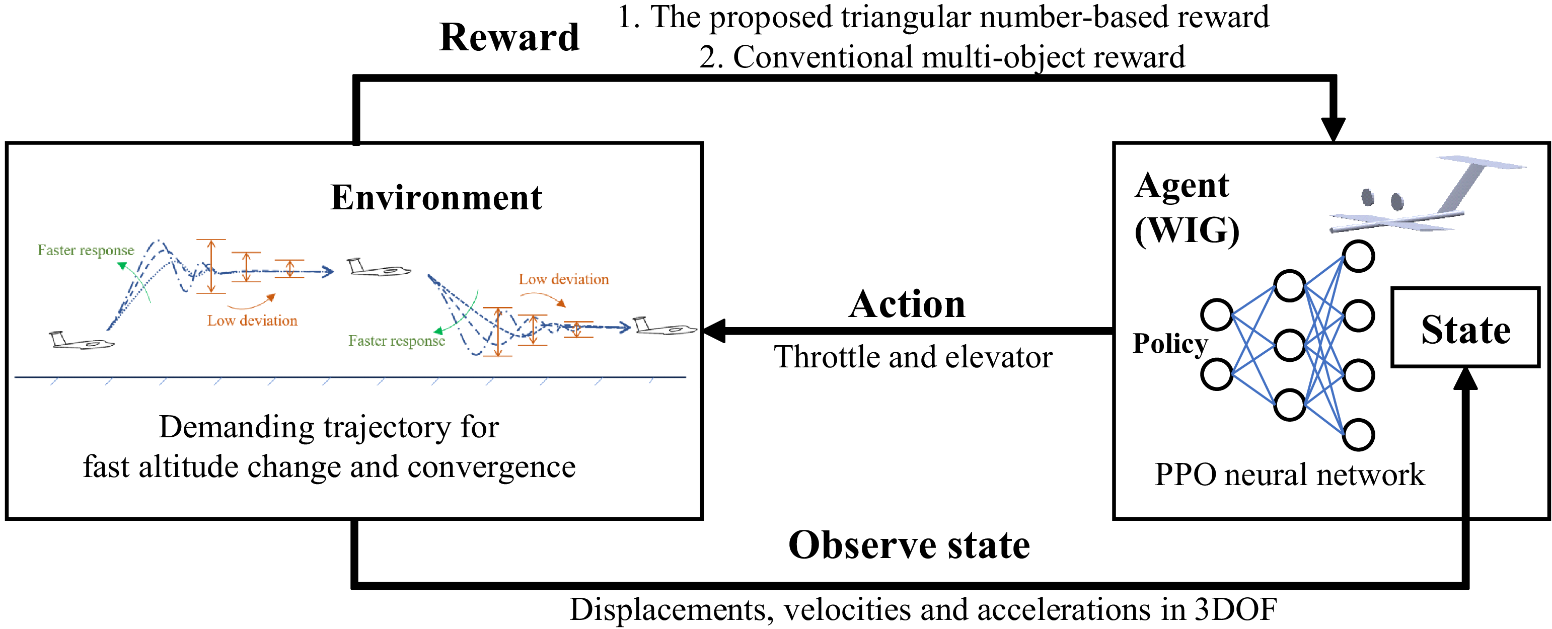
The reward function directs the trajectory towards the extreme value, and therefore, optimisation algorithms are employed to identify this trajectory. Consequently, the identified trajectory is analysed to determine whether it aligns with the design expectations. Deep reinforcement learning (DRL) excels in solving complex, high-dimensional and dynamic decision-making problems by autonomously learning sequential policies. Thus, DRL is utilised as an optimisation tool in this research to search for the trajectory corresponding to the reward function. The basis structure of deep reinforcement learning for WIG’s trajectory planning is shown in Fig. 8. Specifically, the PPO algorithm is employed, and details such as hyperparameters can be found at the link mentioned in the final section Data availability statement . PPO is a policy gradient method that improves stability by limiting the policy update step size. The mathematical formulation of PPO and the corresponding importance sampling mechanism are given in [Reference Schulman, Wolski, Dhariwal, Radford and Klimov35]:
 \begin{align} {L^{CLIP}}\left( \theta \right) &= {\mathbb{\hat{E}}_{t}} [ {{\rm{min}}( {{r_t}\left( \theta \right){{\hat A}_t},{\rm{clip}}\left( {{r_t}\left( \theta \right),1 - \varepsilon ,1 + \varepsilon } \right){{\hat A}_t}} )} ] \\[-10pt] \nonumber\end{align}
 \begin{align} & \qquad \qquad {r_t}\left( \theta \right) = \frac{{{\pi _\theta }\left( {{a_t}|{s_t}} \right)}}{{{\pi _{\theta {\rm{old}}}}\left( {{a_t}|{s_t}} \right)}} \\[10pt] \nonumber \end{align}
where
 $\theta $
denotes the parameters of the policy
 ${\pi _\theta }$
, which defines the probability of taking action
 ${a_t}$
given state
 ${s_t}$
at timestep
 $t$
. The term
 ${\hat A_t}$
represents the estimated advantage at time
 $t$
, quantifying how favourable action
 ${a_t}$
is in state
 ${s_t}$
compared to the expected baseline. It is defined as
 ${\hat A_t}\left( {s,a} \right) = \mathbb{E}\left[ {r\left( {s,a} \right) - r\left( s \right)} \right]$
, where
 $r\left( {s,a} \right)$
denotes the expected reward for taking action
 $a$
in state
 $s$
, and
 $r\left( s \right)$
is the expected reward for state
 $s$
regardless of action. The objective
 $L$
is used to guide gradient ascent updates. The expectation operator
 ${{\hat {\mathbb E}}_t} $
indicates an empirical average over a batch of collected data in the alternating sampling and optimisation process. The ratio
 ${r_t}$
is the importance sampling weight, representing the relative likelihood of the action under the new policy compared to the old one and is essential for stable updates. The function
 ${\rm{clip}}\left( \cdot \right)$
constrains the ratio within a predefined interval to prevent overly large updates; for instance, values below 0 become 0, and those above 1 become 1 when clipped to
 $\left[ {0,1} \right]$
. The hyperparameter
 $\varepsilon $
controls the clipping threshold in the objective function, limiting how far the policy is allowed to deviate during each update. This work implements PPO using ElegantRL [Reference Xiaoyang, Zechu, Zhaoran and Jiahao36], an open-source DRL framework.
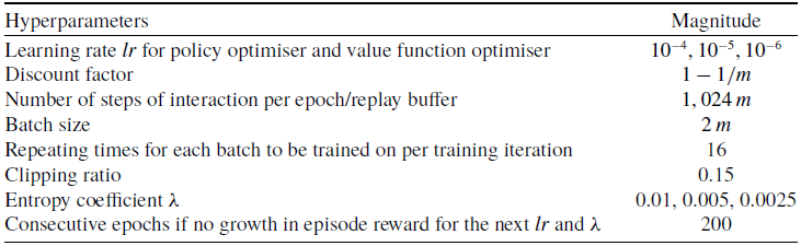
Each DRL case is trained with eight different random seeds, and the training result with the highest reward value is selected as the final outcome for that case. The training hyperparameters are set as follows: each policy iteration collects 1,024 complete trajectory steps of data, with the clip ratio set to 0.15. During training, when the reward showed no improvement after 200 consecutive iterations, the learning rate is reduced from the initial
 ${10^{ - 4}}$
to
 ${10^{ - 5}}$
, and the entropy coefficient is decreased from 0.01 to 0.005. Training then continued until the reward again showed no improvement after another 200 iterations, at which point the learning rate is further reduced to
 ${10^{ - 6}}$
and the entropy coefficient to 0.0025. The training is terminated when no reward improvement is observed for a final 200-iteration period. Table 2 lists hyperparameters of the DRL algorithm.
Hyperparameters of DRL for the adjustment of altitude

Table 2. Long description
The table lists hyperparameters for a deep reinforcement learning algorithm used for altitude adjustment. It has six rows and two columns. The columns are labeled Hyperparameters and Magnitude. The rows are as follows: Row 1: Learning rate for policy optimiser and value function optimiser, 0.0003; Row 2: Discount factor, 0.99; Row 3: Number of steps of interaction per epoch/replay buffer, 1024; Row 4: Batch size, 64; Row 5: Repeating times for each batch to be trained on per training iteration, 16; Row 6: Clipping ratio, 0.15; Row 7: Entropy coefficient, 0.01, 0.005, 0.0025; Row 8: Consecutive epochs if no growth in episode reward for the next and, 200.
The structure of deep reinforcement learning for WIG’s trajectory planning.

4.0 Cases and analysis
To validate the effectiveness of the proposed reward function, the manoeuvre is designed as the switch of the flight altitude from the initial
 ${h_0}$
=0.24 m to the end
 ${h^{\rm{*}}}$
=0.12 m (Fig. 9), and the planned trajectory is compared with those obtained by a conventional multi-objective reward function. The trajectory consists of 24 steps,
 $m$
= 24. The conventional multi-objective reward function is expressed by
 \begin{align} R_e^ \star &= \mathop \sum \limits_{i = 1}^m \left( {1 - \left| {{{{h_i} - {h^{\rm{*}}}} \over {{h^{\rm{*}}} - {h_0}}}} \right|} \right) \\[-10pt] \nonumber\end{align}
 \begin{align} & \quad R_r^ \star = m - {t_r} \\[-9pt] \nonumber \end{align}
 \begin{align} & R^{\star} = R_e^ \star + k \cdot R_r^ \star \\[10pt] \nonumber\end{align}
where
 ${t_r}$
is the order of the step where RT occurs in the trajectory, and
 $k$
is the weight of the RT-related part, which needs to be tuned step by step to roughly obtain the expected trajectory. Likewise,
 $R_e^ \star $
and
 $R_r^ \star $
are the RT and IAE parts of total reward,
 ${R^ \star }$
. Their evaluation is based on all steps, which is the most significant difference from the proposed reward function.
Validation case of a WIG’s flight altitude switch.

4.1 Effectiveness
To validate the effectiveness of the proposed method, we employed a traditional multi-objective function configured with a sequence of seven continuously increasing weight values. This setup simulates the practical process of iteratively tuning weights in multi-objective optimisation until convergence to the target trajectory is achieved. The proposed method is implemented under the same conditions for comparison. The traditional approach uses seven distinct weight values:
 $k = 0$
,
 $k = {10^{ - 2}}$
,
 $k = {10^{ - 1}}$
,
 $k = {10^0}$
,
 $k = {10^1}$
,
 $k = {10^2}$
and
 $k = {10^3}$
, while the proposed method is represented by ‘Proposed’.
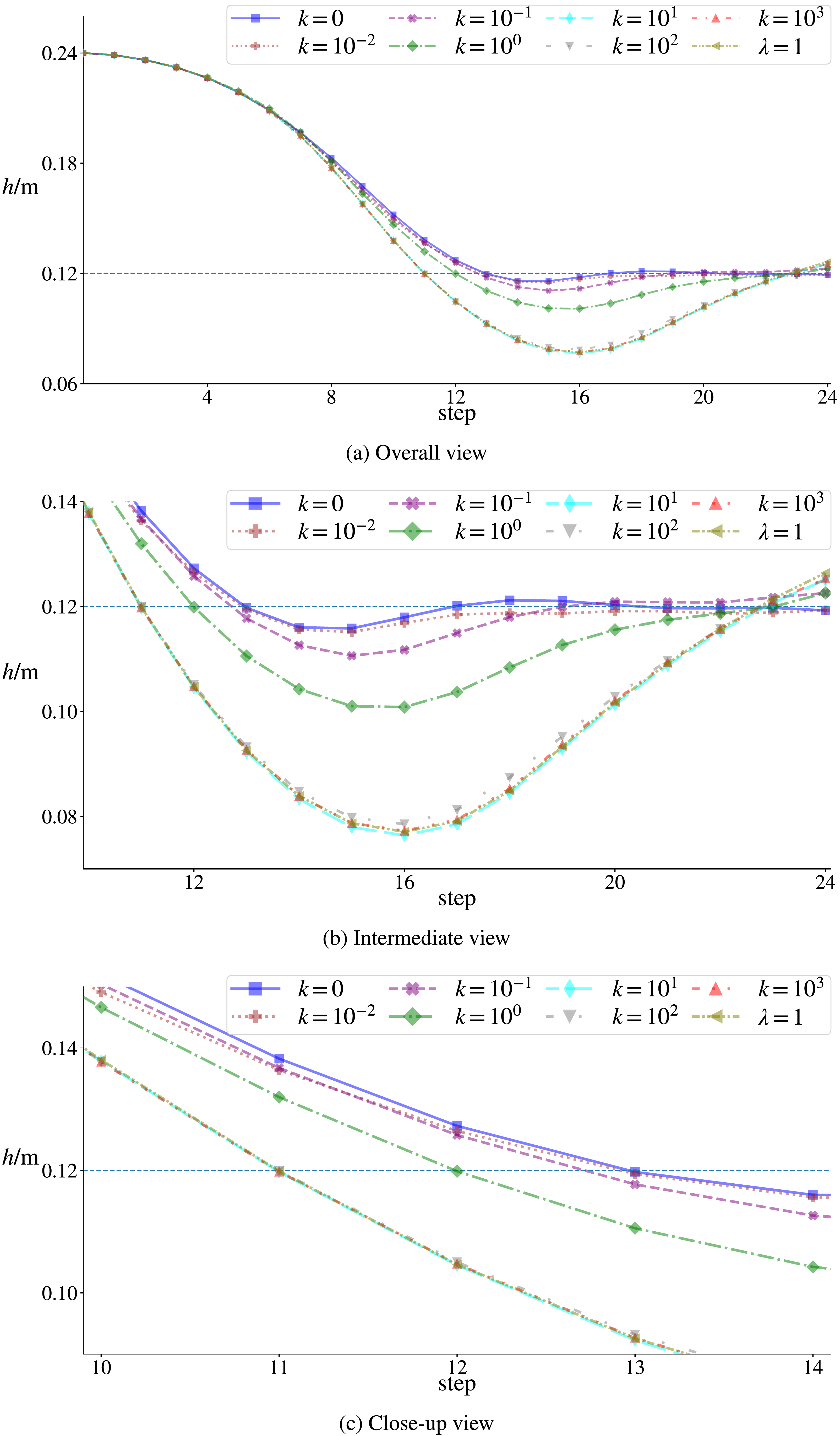
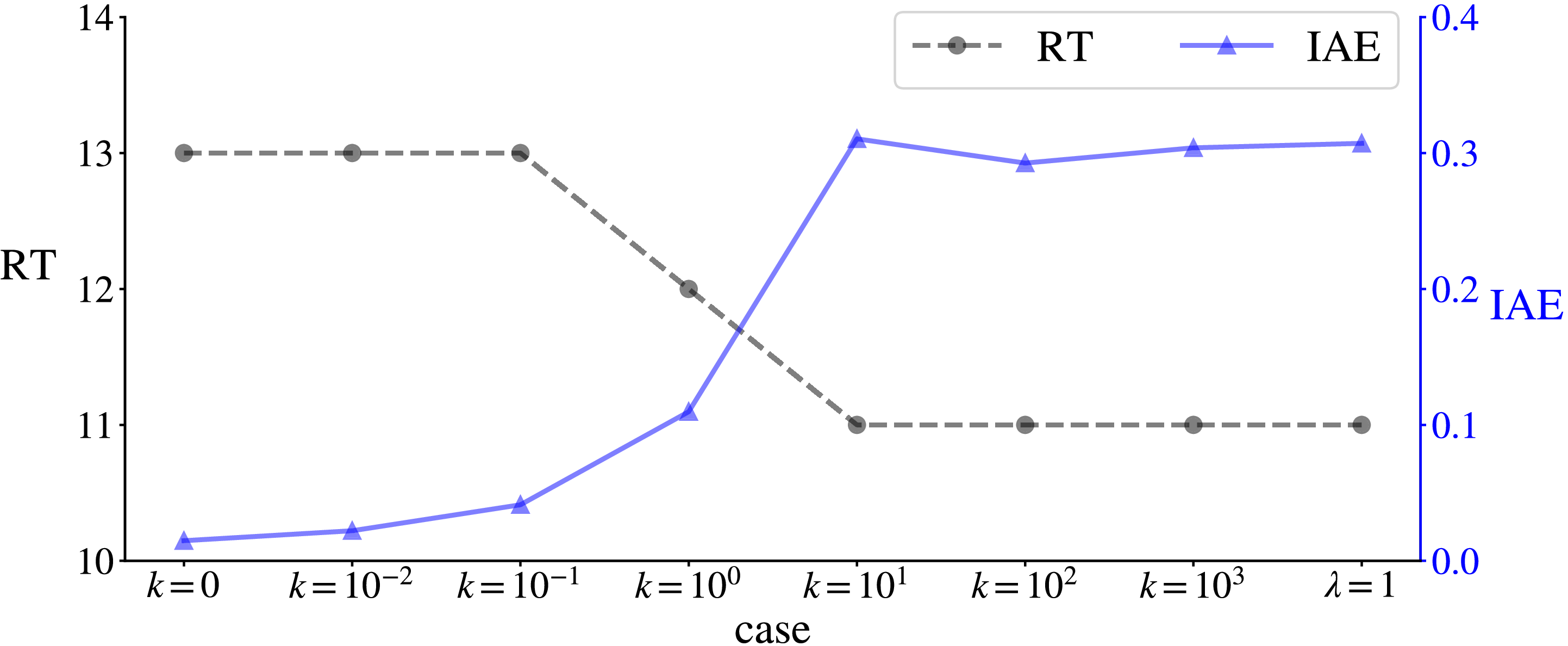
Figure 10 shows the results of the multi-objective reward function with different weight schemes. Figure 10(c) demonstrates that as the RT-related weight increases from
 $k = 0$
to
 $k = {10^1}$
, the moment when the WIG craft reaches the target altitude gradually advances, until the rise time is minimised at the 11-th step. In the latter part of the trajectory, Fig. 10(a) shows that after reaching the target altitude, the concavity of the trajectory becomes increasingly pronounced, accompanied by a corresponding growth in deviation from the target altitude. The degree of concavity reaches its maximum when the RT-related weight increases to
 $k = {10^1}$
. Figure 10(b) further reveals that although trajectory deviation increases with the RT-related weight, this trend saturates once the weight exceeds
 $k = {10^1}$
, beyond which further increases yield no significant change in deviation. The trajectory corresponding to the proposed reward function directly achieves the minimum RT and subsequent approach to the target altitude. The proposed reward function does not introduce any part that needs iterative adjustments of weights through trial and error, and it directly results in the expected trajectory with the maximum concavity.
Trajectories of multi-objective reward functions assigned with different weight
 $k$
and the proposed reward function.

Figure 11 displays the RT and IAE values for the aforementioned cases. It can be observed that as the RT-related weight in the multi-objective function increases exponentially, the trajectory’s RT decreases while the IAE increases. Beyond
 $k = {10^1}$
, both RT and IAE have plateaued, and the proposed method directly achieves identical RT and IAE values. The observed behaviour aligns with the design intent: a relatively large RT-related weight in the reward function effectively reduces RT. The proposed method achieves the same RT and IAE as the multi-objective approach after full convergence, demonstrating that it successfully minimises RT while preventing further increase in IAE, thereby reaching the minimum IAE achievable under the constraint of minimised RT. With increasing RT-related weight, its proportion in the total reward becomes more substantial. Since the WIG tends to maximise reward, its trajectory shows a tendency toward reduced RT, though this comes at the cost of greater deviation from the target altitude. When the RT-related weight is sufficiently large, the reward gain from reducing RT exceeds the loss caused by trajectory deviation, thereby promoting a faster response. This indicates that the earlier arrival at the target altitude is achieved at the expense of trajectory precision during the approach.
Performance of RT and IAE for the multi-objective reward function with different weight
 $k$
and the proposed reward function

4.2 Invariance
The proposed reward function is highly effective in achieving both reduced RT and lower deviation, and its performance is unlikely to be significantly improved through further modifications. To demonstrate the advantage of the proposed reward function over traditional multi-objective approaches that require parameter tuning, an additional coefficient
 $\lambda $
is introduced to examine its invariance, as:
 \begin{align} {R_r} &= 1 + \frac{{n\,{\rm{*}}\left( {n + 1} \right)}}{2}{\rm{\;}},{\rm{\;\;}}n = m - {t_r} \\[-10pt] \nonumber\end{align}
 \begin{align} {R_e} &= \mathop \sum \limits_{i = {t_r}}^m \left( {1 - \left| {{{{h_i} - {h^{\rm{*}}}} \over {{h^{\rm{*}}} - {h_0}}}} \right|} \right) \\[-10pt] \nonumber\end{align}
 \begin{align} R &= {R_e} + \lambda \cdot {R_r} \\[10pt] \nonumber \end{align}
Four coefficients –
 $\lambda = 1$
,
 $\lambda = 10$
,
 $\lambda = {10^1}$
and
 $\lambda = {10^2}$
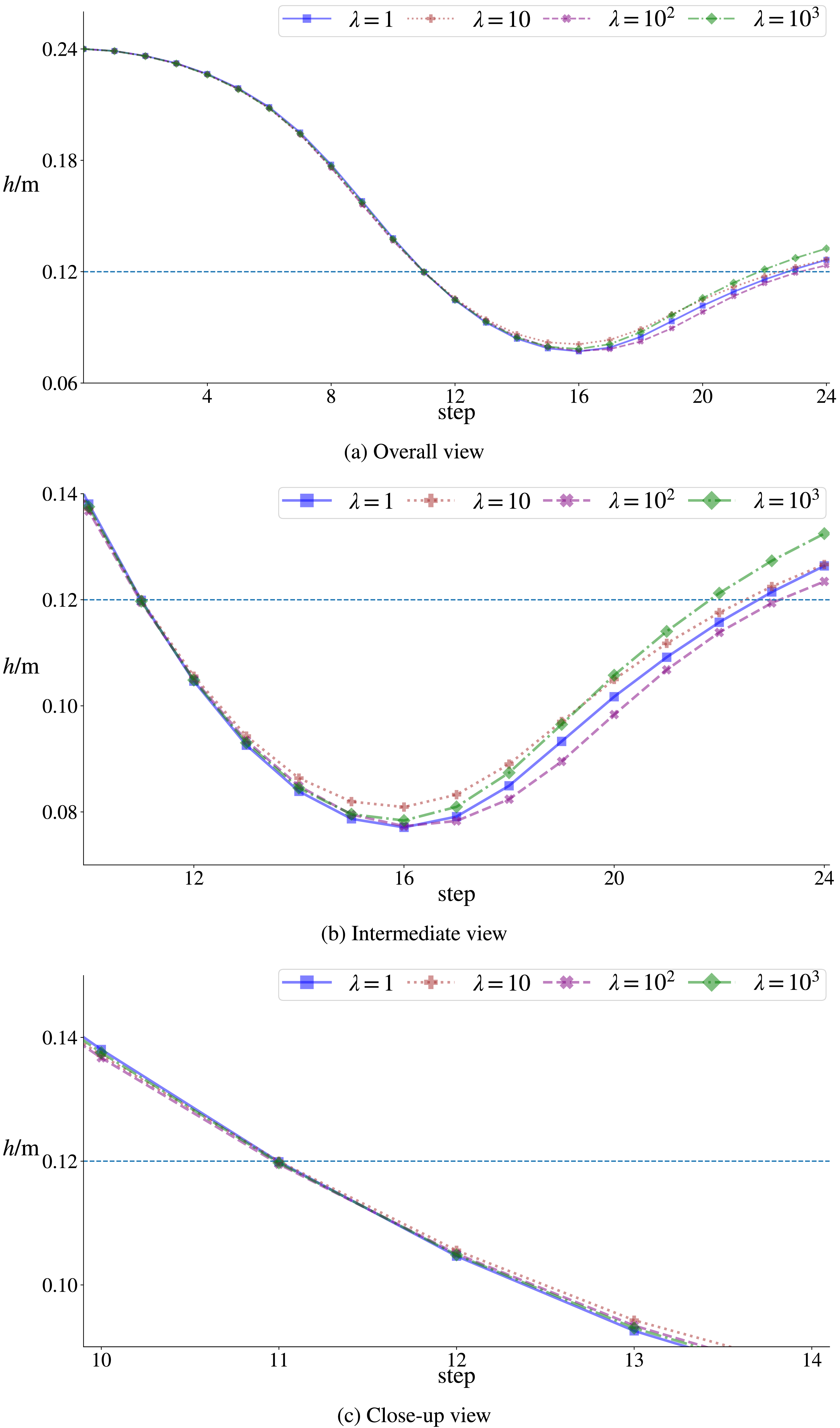
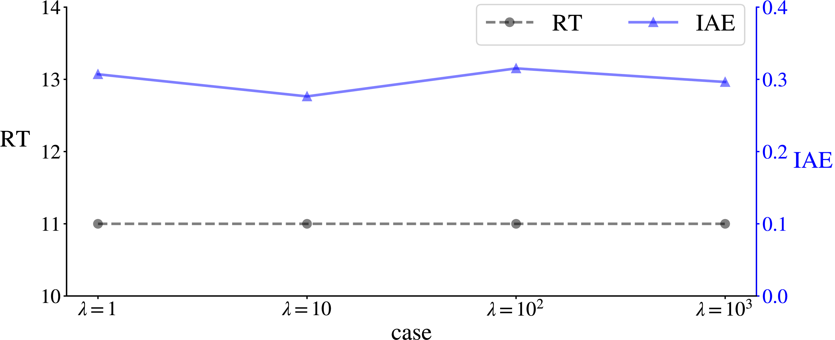
– are selected to compare the resulting trajectories, as shown in Fig. 12. It can be observed that the trajectories are similar. Figure 13 presents the corresponding RT and IAE values, which show only minor differences. Slight variations can be seen in the concavity of the latter trajectory segments, which may be attributed to optimisation errors. This consistency occurs because when
 $\lambda \geqslant 1$
, the reward gain from reducing RT is guaranteed to be sufficiently large to outweigh the penalty caused by increased deviation. Since the quantitative condition of the reward function is satisfied, essentially identical trajectories are obtained.
Trajectories of the proposed reward functions assigned with different coefficient
 $\alpha $
.

Performance of RT and IAE for the proposed reward function with different coefficient
 $\lambda $
.

Validation is performed by attaching a coefficient greater than 1 to the RT-related term and comparatively evaluating a series of coefficient values. The results confirm that the proposed reward function requires no custom development for performance adjustment. Unlike conventional multi-objective reward functions, this method eliminates the need for iterative coefficient tuning and directly generates the ideal trajectory that achieves minimum rise time while maintaining maximum proximity to the target altitude.
5.0 Conclusion
A reward function is proposed to directly achieve rapid response by minimising RT during state transition, allowing the WIG to quickly adjust its flight altitude, and then sufficiently approach the target altitude. The core idea is to set the reward for early RT higher than the penalty for deviating from the target altitude, thus encouraging the WIG to reach the target altitude more quickly. Its effectiveness is validated through trajectory planning of a WIG’s change of flight altitude. By comparison with conventional multi-objective reward functions that adjust weights, the straightforward advantage of the proposed method is highlighted. It can guide the WIG to exert itself to quickly change and converge to the target altitude.
Acknowledgements
The authors gratefully acknowledge the constructive comments from the anonymous reviewers and the editor, whose insights and suggestions significantly improved the quality of this manuscript.
Data availability statement
Source codes are available at the link that is https://github.com/HuanHu2019/Triangular-Numbers-Based-Objective-Function-for-Fast-Altitude-Change-and-Convergence.
Competing interests
The authors declare that they have no known competing financial interests or personal relationships that could have appeared to influence the work reported in this paper.

 t
 t′
 Rr
 Re
 Rr
 Re
 k
 k
 α
 λ


