



1. Introduction
Lift and propulsion mechanisms in fluids have been extensively studied across a wide range of the Reynolds numbers (
 $\textit{Re}$
). At high
 $\textit{Re}$
(
 $\gt 10^4$
), typical of aeronautical applications, the literature is rich with theoretical, computational and experimental insights. Decades of research have established that cambered thin-plate airfoils ensure optimal lift-to-drag ratios for the range of
 $\textit{Re}$
up to
 $10^5$
. Low-
 $\textit{Re}$
regimes (
 $\textit{Re} \ll 1$
), typical of microbial swimmers, have also received substantial attention. Here, the Stokes flow approximation enables analytical solutions yielding explicit formulas for the fluid-dynamic forces. Intermediate
 $\textit{Re}$
values (
 $1 \lesssim \textit{Re} \lesssim 10{\,}000$
), prevalent in biological locomotion, have historically received less attention. This gap likely stems from analytical intractability (viscous and inertial effects compete without simplifying assumptions) and experimental challenges: neither traditional high-
 $\textit{Re}$
wind tunnels nor microfluidic set-ups can reliably cover this range of
 $\textit{Re}$
. Recent technological advances in bio-inspired micro air vehicles have spurred practical interest in this flow regime.
Studies on insect flight (
 $\textit{Re} \sim 10$
–
 $1000$
) often employ flat, cambered or even corrugated thin foils as wing models. Yet, systematic efforts to identify optimal airfoil shapes remain scarce, with most work prioritising kinematics over geometry. A notable exception is the shape-optimisation study by Srinath & Mittal (Reference Srinath and Mittal2009), which explored a broad parameter space of airfoil contours at fixed angles of attack
 $(\alpha = 4^\circ$
and
 $12^\circ )$
using adjoint optimisation. However, the complex shapes obtained therein reflect the
 $\alpha$
constraint rather than the necessity of non-zero thickness. Our present study addresses this problem through a low-dimensional parameterisation of airfoil profiles, enabling efficient exploration of the combined effect of main features of the shape (i.e. thickness and camber) and angle of attack across intermediate
 $\textit{Re}$
. By coupling a parametric geometrical description with Navier–Stokes simulations, we identify optimal airfoils within the Joukowski family, then more general airfoil shapes with adjustable position of the maximum camber. We relate the observed trends of the optimal parameters as functions of
 $\textit{Re}$
to the competing effect of camber-enhanced lift and inertia-driven separation.
2. Mathematical model
2.1. Governing equations
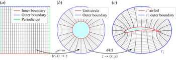
Airfoil optimisation requires flow solutions for many candidate profiles, making repeated mesh generation computationally expensive. We avoid this by using conformal mapping, which simultaneously defines the airfoil, generates an orthogonal grid and yields the metric terms for the transformed Navier–Stokes equations. The map is constructed in two stages, mapping the airfoil exterior to the computational domain via an intermediate annular domain (see figure 1). The starting point is a rectangular grid in
 $(r,s)$
coordinates, where
 $r$
is the radial coordinate and
 $s$
the periodic angular coordinate. The first map,
 $ z = e^{ar + \mathrm{i}as},$
where the parameter
 $a \in \mathbb{R}$
controls the grid stretching, deforms this rectangular grid into an O-grid in the complex
 $z$
-plane: lines of constant
 $r$
become concentric circles, and lines of constant
 $s$
become radial rays. The second map,
 $\phi$
, from the annulus onto the airfoil exterior,
 $ x + \mathrm{i}y = \phi (z),$
deforms the O-grid into a body-fitted mesh, with the inner boundary conforming to the airfoil surface
 $\varGamma$
and the outer boundary mapped to the far-field boundary
 $\varGamma _1$
. We will examine two sets of results using two different maps
 $\phi (z)$
: Joukowski transform (§ 2.3) and Wegmann transform (§ 2.4). With the composite mapping defined, the incompressible steady Navier–Stokes equations in vorticity–streamfunction form can be rewritten in
 $(r,s)$
coordinates. Denoting
 $A = \mathrm{Re}(\phi '(z)az)$
and
 $B = \mathrm{Im}(\phi '(z)az)$
, the Jacobian of the transformation
 $(r,s)\to (x,y)$
is
 $ \unicode{x1D645}= \big(\begin{smallmatrix} A & -B \\ B & A \end{smallmatrix}\big),$
and the governing equations are written in computational coordinates
 \begin{eqnarray} \frac {1}{\det \unicode{x1D645}}\left (\frac {\partial \psi }{\partial s}\frac {\partial \omega }{\partial r} -\frac {\partial \psi }{\partial r}\frac {\partial \omega }{\partial s}\right ) = \frac {1}{\textit{Re}}\frac {1}{\det \unicode{x1D645}}{\nabla} ^2_{r,s}\omega, \end{eqnarray}
 \begin{eqnarray} \omega = -\frac {1}{\det \unicode{x1D645}}{\nabla} ^2_{r,s}\psi, \end{eqnarray}
where
 $\omega$
is the vorticity,
 $\psi$
is the streamfunction,
 $\textit{Re} = \rho U_\infty c / \mu$
,
 $\rho$
is the fluid density,
 $U_\infty$
the free-stream velocity,
 $c$
the chord length and
 $\mu$
the dynamic viscosity.
The three-stage conformal mapping: (a) rectangular computational domain in
 $(r,s)$
coordinates; (b) intermediate annular domain in the
 $z$
-plane; (c) physical domain with the body-fitted grid to the airfoil surface. Inner and outer boundaries are shown in red and blue, respectively.

Figure 1. Long description
Panel A: A rectangular computational domain in coordinates. The domain is divided into a grid with an inner boundary marked in red, an outer boundary marked in blue, and a periodic cut marked in green. Panel B: An intermediate annular domain in the zeta-plane. The domain is circular with a unit circle marked in red and an outer boundary marked in blue. Panel C: A physical domain with a body-fitted grid to the airfoil surface. The domain includes an airfoil marked in red and an outer boundary marked in blue.
2.2. Boundary conditions
On the airfoil surface
 $\varGamma$
, the no-penetration and no-slip conditions are
 $\partial \psi /\partial \boldsymbol{n} = 0$
and
 $\partial \psi /\partial \boldsymbol{\tau } = 0$
, where
 $\boldsymbol{n}$
and
 $\boldsymbol{\tau }$
denote the unit normal and unit tangent vector to
 $\varGamma$
, respectively. Since conformal maps preserve orthogonality, the conditions retain their form in
 $(r,s)$
coordinates. From the boundary condition
 $\partial \psi / \partial s = 0$
on
 $\varGamma$
, it follows that
 $\psi$
is uniform on the airfoil surface. Since
 $\psi$
is defined only up to an additive constant, this value may be chosen as zero, reducing the boundary conditions to
 $\psi = 0$
and
 $\partial \psi / \partial r = 0$
on
 $\varGamma$
.
At the outer boundary
 $\varGamma _1$
, uniform horizontal free-stream conditions are imposed, which in terms of the streamfunction read
 $\partial \psi /\partial y = 1,\ \partial \psi /\partial x = 0$
on
 $\varGamma _1$
. Applying the chain rule for the conformal transformation yields the outer boundary conditions
 \begin{align} \psi _r = B, \quad \psi _s = A \quad \text{on } \quad \varGamma _1. \end{align}
At the continuous level, both conditions (2.3) are valid and equivalent representations of the imposed far-field velocity. However, in the discrete formulation, prescribing both streamfunction derivatives simultaneously leads to an ill-conditioned system when coupled with the Poisson equation (2.2). Condition (2.3a
) is retained as it directly controls the mass flux through the outer boundary, whereas condition (2.3b
) is redundant given the irrotationality of the undisturbed free stream and therefore dropped in favour of the vorticity condition
 $\omega = 0$
. This substitution restores well-posedness of the discrete system without altering the physical model, yielding the system
 \begin{equation} \begin{aligned} \left (\frac {\partial \psi }{\partial s}\frac {\partial \omega }{\partial r} - \frac {\partial \psi }{\partial r}\frac {\partial \omega }{\partial s}\right ) & = \frac {1}{\textit{Re}}{\nabla} ^2_{r,s}\omega, \\ \omega & = -\frac {1}{\det \unicode{x1D645}}{\nabla} ^2_{r,s}\psi, \end{aligned} \quad \text{with B.C.}\quad \begin{aligned} \psi & = 0, \quad \frac {\partial \psi }{\partial r} = 0 & & \text{on }\varGamma, \\ \frac {\partial \psi }{\partial r} & = B, \quad \omega = 0 & & \text{on }\varGamma _1. \end{aligned} \end{equation}
2.3. Joukowski conformal map
The Joukowski map is defined on the exterior of the unit disk (
 $\mathbb{C}\setminus D_1$
) by analytic formula
 $\widetilde {\phi (z)} = z + z_0 + k^2/(z + z_0)$
, where three real-valued parameters fully determine the airfoil shape:
 $k \geq 0$
controls the thickness,
 $\mu _x = \mathrm{Re}(z_0)$
controls the trailing-edge geometry and
 $\mu _y = \mathrm{Im}(z_0)$
introduces camber. Despite this low-dimensional parameterisation, Joukowski airfoils represent a wide variety of streamlined shapes. This is an analytical mapping, therefore its numerical evaluation is computationally highly efficient and precise.
Since conformality requires a non-zero derivative throughout the domain, constraints on
 $k$
and
 $z_0$
must be imposed. For a conformal map from the exterior of the unit disk to the exterior of the airfoil, two conditions must hold: the shifted centre
 $z_0$
must lie inside the unit disk, ensuring that the denominator
 $z + z_0$
is non-vanishing in
 $\mathbb{C}\setminus D_1$
, and
 $\widetilde {\phi '(z)} \neq 0$
throughout
 $\mathbb{C}\setminus D_1$
.
Preliminary computations over the full parameter space, consistent with Sunada et al. (Reference Sunada, Sakaguchi and Kawachi1997), confirm that an airfoil with a cusped trailing edge (
 $\mu _x \leq 0$
) and upward camber (
 $\mu _y \geq 0$
) achieves higher performance metrics; the parameter space is therefore restricted to
 \begin{equation} \mu _x \in [-1,0],\quad \mu _y \in [0,\sqrt {1-\mu _x^2}\ ),\quad k \in [0, \sqrt {1-\mu _y^2} - |\mu _x| \ ). \end{equation}
The airfoil thickness decreases monotonically as
 $k$
increases toward its upper bound; in the limit
 $k \to \sqrt {1 - \mu _y^2} - |\mu _x|$
the airfoil degenerates to a flat plate.
Two further operations complete the map definition: normalisation to the unit chord and introduction of the angle of attack
 $\alpha$
. Defining
 $c = |z_{x_{\textit{max}}} - z_{x_{\textit{min}}}|$
as the distance between the leftmost and rightmost points, which coincides with the chord length for the thin airfoils considered here, the normalised map is
 $ \widehat {\phi (z)} := \widetilde {\phi (z)} / c.$
The angle of attack
 $\alpha$
is then introduced by composing
 $\widehat {\phi }$
with a rigid rotation:
 $ \phi (z) := \widehat {\phi (z)}\mathrm{e}^{{i}\alpha }.$
The composite normalised Joukowski map, with
 $\alpha$
as an additional parameter, thus takes the form
 \begin{equation} \phi (z) = \frac {e^{{i}\alpha }}{|z_{x_{\textit{max}}} - z_{x_{\textit{min}}}|} \left ( z + z_0 + \frac {k^2}{z + z_0} \right )\!, \end{equation}
with the parameter constraints given by (2.5).
2.4. Wegmann transform
Joukowski mapping provides control over the two most important geometric parameters: thickness and camber. However, it does not allow independent variation of the chordwise position of maximum camber
 $p$
, which is known to be a third key parameter for thin airfoils. To investigate the effect of
 $p$
, we generate the target profile from a four-parameter family and compute the corresponding map numerically following Wegmann (Reference Wegmann1986).
The airfoil is parametrised similarly to NACA profiles. The mean camber line
 $y_c(x)$
, with maximum camber
 $f$
at chordwise position
 $p$
is defined as
 \begin{equation} y_c(x) = \begin{cases} \dfrac {f}{p^2}\bigl (2px - x^2\bigr ), & x \lt p, \\[9pt] \dfrac {f}{(1-p)^2}\bigl (1 - 2p + 2px - x^2\bigr ), & x \geq p, \end{cases} \end{equation}
and a symmetric thickness distribution
 $y_t(x)$
is added normal to it. The thickness follows the NACA four-digit polynomial, with a factor
 $(1-x)^{q-1}$
controlling trailing-edge closure
 \begin{align} y_t(x) = \frac {t}{0.2}\,(1-x)^{q-1}\bigl (0.2969\sqrt {x} - 0.1260\,x - 0.3516\,x^2 + 0.2843\,x^3 - 0.1015\,x^4\bigr ). \end{align}
The exponent
 $q$
controls the trailing-edge shape:
 $q=1.5$
gives a Joukowski-like cusp,
 $q=1$
the wedge of the standard NACA series. We fix
 $t = 0.01$
and
 $q = 1.5$
throughout, leaving
 $(f, p, \alpha )$
as free parameters. The resulting profiles have the leading-edge radius of
 ${\approx} 0.011\,\%$
of the chord length and the maximum thickness near the leading edge of
 ${\approx} 1.2\,\%$
of the chord length. The map is then computed in two steps. First, the inverse Kármán–Trefftz map is computed
 \begin{equation} \frac {z-1}{z+1} = \left (\frac {w-1}{w+1}\right )^{1/n}, \quad n = 2 - \frac {\tau }{\pi }, \end{equation}
with
 $\tau$
defining the trailing-edge wedge angle, which the algorithm measures from the surface tangents at the trailing edge of each profile. For the cusped trailing edges considered here (
 $q = 1.5$
),
 $\tau$
is small and the exponent is close to
 $2$
. This map removes the trailing-edge corner and deforms the airfoil
 $\varGamma$
into a smooth near-circular contour
 $\eta (s)$
parametrised by arclength
 $s \in [0, 2\pi )$
. Second, Wegmann’s algorithm computes the exterior map
 $g$
from the unit circle onto this near circle. The map must project each boundary point
 $\mathrm{e}^{{i}t}$
to a point on the contour
 \begin{equation} g(\mathrm{e}^{{i}t}) = \eta (S(t)), \end{equation}
where the boundary correspondence
 $S(t)$
is the unknown. Requiring
 $g$
to be analytic outside the unit circle turns (2.10) into a nonlinear equation for
 $S(t)$
, which Wegmann’s method solves by iteration. The converged map is represented as a Laurent series,
 $g(w) = m_0 w + \sum _{k=0}^{\infty } c_k\, w^{-k}$
, of which we retain the first
 $80$
coefficients. Composing
 $g$
with the forward Kármán–Trefftz transformation (2.9) results in the conformal map from the exterior of the unit circle directly onto the exterior of the airfoil, yielding
 $\phi (z)$
analogous to the Joukowski map of § 2.3.
2.5. Numerical method
The nonlinear system (2.4) is solved by Newton–Raphson iteration with backtracking line search. Because convergence is sensitive to the initial guess, different initialisation procedures are used for low and high Reynolds numbers. For
 $\textit{Re} \lt 200$
, the potential-flow solution is used as the initial guess. For higher
 $\textit{Re}$
, a continuation strategy is employed over an increasing sequence of Reynolds numbers,
 $\textit{Re}_1 \lt \textit{Re}_2 \lt {\cdots} \lt \textit{Re}_{\textit{target}}$
, with each converged solution used for the next step. As an example, to reach
 $\textit{Re} = 1000$
, the sequence
 $200 \to 300 \to 500 \to 750 \to 1000$
is used.
The linearised system is discretised with second-order finite differences on a uniform
 $N_r \times N_s = 450 \times 600$
grid with a periodic boundary condition in the circumferential direction. The outer boundary is placed at the distance of
 $114c$
and
 $78c$
away from the airfoil for
 $\textit{Re} \lt 150$
and
 $\textit{Re} \geq 150$
, respectively, where the larger domain compensates for the slower decay of velocity perturbations in the low-
 $\textit{Re}$
regime (Khalili & Liu Reference Khalili and Liu2017). The conformal stretching concentrates nodes near the wall: the first off-wall layer thickness ranges from
 $1.3 \times 10^{-4}c$
near the trailing-edge cusp to
 $7.0 \times 10^{-3}c$
along the remainder of the chord. Solver accuracy is confirmed in Appendix.
Once the vorticity–streamfunction system is solved, the lift and drag coefficients are recovered from the surface pressure
 $P$
and wall shear stress
 $\tau _w$
. We use the non-dimensionalisation
 $\rho _\infty = 1$
,
 $U_\infty = 1$
,
 $c = 1$
, under which the dynamic pressure is
 $q_\infty = 1/2,$
dynamic viscosity is
 $\mu = 1/ \textit{Re}$
and the lift and drag coefficients reduce to
 $C_L = 2F_L$
,
 $C_D = 2F_D$
, where
 $F_L$
and
 $F_D$
are lift and drag forces.
The surface pressure satisfies
 $\mathrm{d}P/\mathrm{d}s = -(1/ \textit{Re})(\partial \omega /\partial r)|_{\varGamma }$
, which is obtained from the tangential momentum equation at the wall, with gauge condition
 $\int _\varGamma P\,\mathrm{d}s = 0$
. The wall shear stress is
 $\tau _w = \omega \sqrt {\det \boldsymbol{J}}/ \textit{Re}$
. The lift and drag coefficients follow from integrating the pressure and shear-stress contributions over the airfoil surface, with the Jacobian components
 $A$
and
 $B$
entering through the coordinate transformation
 \begin{equation} C_D = -2\int _\varGamma \textit{PA}\:\mathrm{d}s - \frac {2}{\textit{Re}}\int _\varGamma \omega B \:\mathrm{d}s, \quad C_L = -2\int _\varGamma \textit{PB}\:\mathrm{d}s + \frac {2}{\textit{Re}}\int _\varGamma \omega A \:\mathrm{d}s. \end{equation}
3. Optimisation
We optimise airfoil profiles over
 $\textit{Re} \in [1, 3000]$
in two independent sets of numerical experiments to maximise two different performance metrics:
 $C_L/C_D$
(in the literature termed as lift-to-drag ratio, or glide ratio) and
 $C_L^{3/2}/C_D$
(termed as endurance factor, or power factor). These are the two most commonly used objectives when designing airfoils for regimes that typically constitute most of the flight duration, e.g. cruise and loitering flight. Since direct search over the full four-parameter space
 $(k, \mu _x, \mu _y, \alpha )$
, as defined in (2.6), is computationally expensive, we progressively narrow the parameter domain as follows.
We begin by analysing symmetric airfoils:
 $\mu _y = 0$
,
 $\mu _x = 0$
. This reduction to a two-parameter problem (
 $k,\alpha$
) makes it feasible to construct the objective function over a structured grid and examine its global behaviour. The computed objective surfaces reveal that, within the class of symmetric airfoils, the highest performance is consistently achieved for zero-thickness airfoils, corresponding to a flat plate. To determine whether this tendency persists when camber and trailing-edge geometry are free, we proceed to the full four-parameter space of Joukowski foils, employing three complementary global search strategies in parallel: Sobol sequence sampling, covariance matrix adaptation evolution strategy and Bayesian optimisation. All three strategies consistently identify zero-thickness airfoils with
 $\mu _x \approx 0$
as optimal across the entire
 $\textit{Re}$
range, in agreement with existing results for low-Reynolds-number airfoils (Sunada et al. Reference Sunada, Sakaguchi and Kawachi1997). Accordingly, the parameter
 $\mu _x$
is set to
 $0$
and
 $k$
is set to the zero-thickness limit for each
 $\mu _y$
, as given by the upper bound in (2.5). This reduction implies
 $k = \sqrt {1 - \mu _y^2}$
(in practice,
 $k$
is set to
 $\sqrt {1-\mu _y^2} - \varepsilon$
with
 $\varepsilon = 10^{-7}$
to avoid the map singularity at the boundary of the admissible domain; this has no measurable effect on the aerodynamic coefficients), leaving
 $\mu _y$
as the only geometric parameter of the airfoil. For a thin Joukowski profile,
 $\mu _y$
is related to the camber
 $f$
through the image of the top of the circle (
 $z = \mathrm{i}$
)
 \begin{equation} f = \mathrm{Im} \big( \mathrm{i} + \mu _y\mathrm{i} + \big(1 - \mu _y^2 \big)/(\mathrm{i} + \mu _y\mathrm{i}) \big )/c = \mu_y/(2k), \end{equation}
which inverts to give
 $\mu _y = 2f/\sqrt {1 + 4f^2}.$
The optimisation thus reduces to a two-parameter problem in
 $(f, \alpha )$
space. A structured high-resolution grid search is performed over this plane with steps
 $\Delta \alpha = 0.5^\circ$
and
 $\Delta f = 0.5\,\%$
, within windows centred on the regions identified by the global search.
4. Results and discussion
Let us denote as
 $\alpha _{\textit{opt},G}$
and
 $f_{\textit{opt},G}$
, respectively, the angle of attack and camber that maximise
 $C_L/C_D$
. Similarly,
 $\alpha _{\textit{opt},E}$
and
 $f_{\textit{opt},E}$
will stand for the values that maximise
 $C_L^{3/2}/C_D$
. We will also use shorter notations
 $\alpha _{\textit{opt}}$
and
 $f_{\textit{opt}}$
in statements that apply to both maximisation objectives. The results of the high-resolution grid search optimisation are presented in figure 2. Solid lines correspond to the Joukowski airfoils. Point markers correspond to the extended optimal shapes obtained with the position of the maximum camber
 $p$
as an additional optimisation parameter, by employing a Wegmann transform. For both airfoil families and both objective functions, the results are qualitatively the same and quantitatively close. Let us first discuss the results obtained for Joukowski airfoils. As
 $\textit{Re}$
increases from
 $1$
to
 $3000$
,
 $\alpha _{\textit{opt}}$
decreases monotonically from
 $39^\circ$
to
 $6^\circ$
, with a maximum difference between
 $\alpha _{\textit{opt},E}$
and
 $\alpha _{\textit{opt},G}$
of
 $3.2^\circ$
at
 $\textit{Re} = 50$
. The parameter
 $f_{\textit{opt}}$
follows a bell-shape curve, with
 $f_{\textit{opt},G}$
and
 $f_{\textit{opt},E}$
behaving nearly identically at the boundaries of the
 $\textit{Re}$
range considered: starting and ending at
 $3.5\,\%$
at
 $\textit{Re} = 1$
and
 $\textit{Re} = 3000$
. Significant differences appear only near the peaks:
 $f_{\textit{opt},G} = 12.3\,\%$
at
 $\textit{Re} = 40$
and
 $f_{\textit{opt},E} = 15.2\,\%$
at
 $\textit{Re} = 50$
, and a maximum difference of
 $2.9\,\%$
at
 $\textit{Re} = 50$
.
Results of optimisation of
 $C_L/C_D$
(subscript
 $G$
) and
 $C_L^{3/2}/C_D$
(subscript
 $E$
). (a) Optimal angle of attack
 $\alpha _{\textit{opt}}$
as a function of
 $\textit{Re}$
; (b) optimal camber
 $f_{\textit{opt}}$
as a function of
 $\textit{Re}$
; (c) optimal chordwise position
 $p_{\textit{opt}}$
of the maximum camber as a function of
 $\textit{Re}$
; (d) maximum
 $C_L/C_D$
and
 $C_L^{3/2}/C_D$
as functions of
 $\textit{Re}$
. Solid blue and red lines and the letter J correspond to the results obtained for Joukowski airfoils. Green and yellow triangular markers and the letter W correspond to the results of calculations using the Wegmann method with the chordwise position
 $p$
of the maximum camber treated as one of the optimisation parameters. Black dotted lines and letter M represent the asymptotic formula for the maximum
 $C_L^*/C_D^*$
value and corresponding
 $\alpha _{opt,*}$
for a flat plate. The position of the maximum camber of thin Joukowski foils is constrained at
 $p=50\,\%$
and therefore not shown on the plot.

When the position
 $p$
of the maximum camber is treated as an adjustable parameter, for the flow regimes near
 $\textit{Re} = 10$
, the optimal position of the maximum camber is near 50 % chordwise. However, for larger
 $\textit{Re}$
, optimal position of the maximum camber progressively shifts downstream toward the trailing edge. The cambers
 $f$
are larger but the angles of attack
 $\alpha$
are the same as for the Joukowski airfoils. The objective function values are slightly greater than for the Joukowski airfoils. The latter results, however, have been obtained with the fixed maximum thickness near the leading edge of 1.2 % of the chord length as required for the numerical mapping, and this value is considerably larger than the Joukowski airfoil thickness. It can be postulated that trends shown in figure 2 might be generally representative of optimal thin airfoils.
In the low-Reynolds-number regime, the Oseen approximation is valid, and the numerical results show that
 $f_{\textit{opt}} \to 0$
, meaning the optimal shape reduces to a flat plate. It is therefore natural to compare the numerical results against the analytical solution derived by Miyagi (Reference Miyagi1964) for the lift and drag of a flat plate under the Oseen approximation:
 $ C_D^* = ({16\pi }/{\textit{Re}})(({2S_1 - 1 - \cos 2\alpha)}/{(4S_1^2 - 2(1+\cos 2\alpha)})), \quad C_L^* = ({16\pi }/{\textit{Re}}) (({\sin 2\alpha})/{(4S_1^2 - 2(1+\cos 2\alpha )})),$
where
 $S_1 = \ln (16/ \textit{Re}) - \gamma$
, with
 $\gamma$
denoting the Euler–Mascheroni constant. Maximising
 $C_L^*/C_D^*$
with respect to
 $\alpha$
yields the optimal angle,
 $\alpha _{opt,*} = \arctan \sqrt {1 - 1/S_1}$
, which satisfies
 $\alpha _{opt,*} \to 45^\circ$
as
 $\textit{Re} \to 0$
, explaining the large optimal angles of attack observed at the lower end of the Reynolds-number range. Since
 $S_1$
is a decreasing function of
 $\textit{Re}$
,
 $\alpha _{opt,*}$
itself decreases monotonically with
 $\textit{Re}$
, consistent with the numerical results.
The non-monotonic behaviour of
 $f_{\textit{opt}}$
arises from a competition between positive and negative aerodynamic effects. The benefits of non-zero camber are twofold. First, curvature enhances the inertial pressure differential between lower and upper surfaces. Second, these enhanced pressure forces near the leading edge are oriented vertically, contributing to
 $C_L$
to a greater extent. On the downside, greater pressure differential on a cambered foil entails larger adverse pressure gradient in the aft portion of it, which leads to flow separation and increased drag. As
 $\textit{Re}$
increases from the lower end, increased inertia boosts the curvature-induced excess
 $C_L$
. At the same time, viscous diffusion remains strong enough to mitigate flow separation even at large
 $f$
and
 $\alpha$
, permitting highly cambered airfoils to remain near optimal. Together, these effects drive
 $f_{\textit{opt}}$
upward until
 $\textit{Re} \approx 40{-}50$
.
Beyond this peak, the trend reverses: as inertia becomes dominant, viscosity can no longer resist and the flow separates at large
 $f$
and
 $\alpha$
without reattachment. Both
 $f_{\textit{opt}}$
and
 $\alpha _{\textit{opt}}$
decline toward lower values. Flow detachment simultaneously reduces lift and increases drag, impairs both
 $C_L/C_D$
and
 $C_L^{3/2}/C_D$
; any
 $(f, \alpha )$
combination at which the bubble opens is suboptimal. The optimal airfoils, therefore, reside in the attached-flow regime, which justifies the use of the steady solver in this study. At
 $\textit{Re} = 100$
, the optimal cambered airfoil (
 $f_{\textit{opt},G} = 11.2\,\%, \, \alpha = 16.6^\circ$
) already carries a trailing-edge recirculation bubble, visible in the streamlines (figure 3
b,c), yet the flow remains steady. This airfoil achieves
 $17\,\%$
higher
 $C_L/C_D$
than the flat plate (figure 3
a,d), confirming that moderate camber remains beneficialeven as a separation bubble begins to form. For the optimal shape found at
 $\textit{Re}=3000$
(
 $f_{\textit{opt},G} = 3.5\,\%$
,
 $\alpha = 6 ^\circ$
), this was confirmed by supplementary unsteady numerical simulations using OpenFOAM (see https://osf.io/y4pr8), in which the fluctuation amplitude did not exceed 0.2 % of the respective mean values. The Reynolds number based on the perpendicular projection of the chord,
 $\textit{Re}_\perp = \textit{Re} \sin \alpha$
, equals 314 in the optimal case at
 $\textit{Re} = 3000$
, and decreases with the decreasing
 $\textit{Re}$
, further supporting the steady flow assumption.
(a) Lift, drag and lift-to-drag ratio curves as functions of
 $\alpha$
at
 $\textit{Re} = 100$
for the flat and optimal cambered profiles, with optimal
 $\alpha$
and values of
 $C_L/C_D$
marked. (b,c) Streamlines for the optimal cambered and flat profiles respectively, shown at levels
 $0,\pm 10^{-5}, \pm 5\times 10^{-5}, \pm 10^{-4}, \pm 5\times 10^{-4}, \pm 10^{-3}$
. (d) Pressure coefficient difference along the chord for both profiles.

Figure 3. Long description
Panel A: A line graph shows aerodynamic coefficients as functions of the angle of attack for flat and cambered profiles. The x-axis represents the angle of attack in degrees, and the y-axis represents the aerodynamic coefficients. The graph includes multiple lines representing different coefficients for flat and cambered profiles, with optimal values marked by horizontal and vertical dashed lines. Panel B: A line graph displays streamlines for the optimal cambered profile at specific levels. The x-axis represents the x-coordinate, and the y-axis represents the y-coordinate. Panel C: A line graph shows streamlines for the flat profile at specific levels. The x-axis represents the x-coordinate, and the y-axis represents the y-coordinate. Panel D: A line graph illustrates the pressure coefficient difference along the chord for both flat and cambered profiles. The x-axis represents the x-coordinate, and the y-axis represents the pressure coefficient difference. The graph includes lines for both profiles, with a legend indicating which line corresponds to each profile.
At low
 $\textit{Re}$
, strong viscous diffusion spreads the
 $C_L/C_D$
and
 $C_L^{3/2}/C_D$
maxima broadly across the
 $(f, \alpha )$
space; as inertia strengthens with
 $\textit{Re}$
, the maxima sharpen, making a geometrically precise optimal airfoil identifiable. This is illustrated in figure 4, which shows contour plots of
 $C_L/C_D$
at
 $\textit{Re} = 10, 100$
and
 $500$
. All panels span equal ranges
 $\delta f \times \delta \alpha = 7\,\% \times 10^\circ$
, centred on
 $(f_{\textit{opt}}, \alpha _{\textit{opt}})$
at each
 $\textit{Re}$
, enabling direct comparison of landscape sharpness. At
 $\textit{Re} = 10$
,
 $C_L/C_D$
varies by less than
 $5\,\%$
across the displayed range, meaning that a wide number of
 $(f, \alpha )$
combinations yields nearly identical performance. As
 $\textit{Re}$
increases, the maximum becomes more distinct: at
 $\textit{Re} = 100$
the variation reaches
 $10\,\%$
, and at
 $\textit{Re} = 500$
it is
 $25\,\%$
. This progressive sharpening has a direct implication: below
 $\textit{Re} \approx 100$
, performance is insensitive to the precise choice of
 $f$
and
 $\alpha$
, whereas above
 $\textit{Re} \approx 500$
, the sharp peak singles out a physically distinguished
 $(f, \alpha )$
combination, making optimisation both meaningful and effective.
Counterplots of
 $C_L/C_D$
normalised by its maximum value, in the
 $(f, \alpha )$
parameter space: (a) for
 $\textit{Re} = 10$
; (b) for
 $\textit{Re} = 100$
; (c) for
 $\textit{Re} = 500$
. Stars mark the
 $(f^*, \alpha ^*)$
in each case. All panels span equal areas of the
 $(f, \alpha )$
parameter space.

5. Conclusion
Optimisation of Joukowski airfoils across
 $\textit{Re} \in [1, 3000]$
within the steady, laminar, incompressible Navier–Stokes model has revealed features and trends of optimal airfoils that are common to both the
 $C_L/C_D$
and
 $C_L^{3/2}/C_D$
maximisation in the intermediate-Reynolds-number range. Zero-thickness cambered airfoils are optimal for both
 $C_L/C_D$
and
 $C_L^{3/2}/C_D$
throughout the entire intermediate-
 $\textit{Re}$
range. This result is confirmed by three independent global search strategies. The optimal angle of attack decreases monotonically with
 $\textit{Re}$
, while the optimal camber follows a bell-shaped curve. At
 $\textit{Re} \lesssim 10$
, near-flat plates (
 $f \lesssim 11\,\%$
) at high angle of attack (
 $\alpha \approx 35{-}39^\circ$
) are optimal. As
 $\textit{Re}$
increases, optimal camber attains a peak of
 $12.3\,\%$
(
 $C_L/C_D$
) and
 $15.2\,\%$
(
 $C_L^{3/2}/C_D$
) at
 $\textit{Re} \approx 40{-}50$
, marking the transition from viscosity-dominated to inertia-dominated flow. At
 $\textit{Re} = 3000$
, both
 $f$
and
 $\alpha$
converge toward the slightly cambered (
 ${\sim }4\,\%$
) low-
 $\alpha$
(
 ${\sim }6^\circ$
) geometry, in close agreement with the optimal airfoils identified by Sunada et al. (Reference Sunada, Sakaguchi and Kawachi1997) at
 $\textit{Re} = 4000$
and consistent with the slightly cambered geometry characteristic of conventional low-speed airfoils. Another useful property is the sharpness of the
 $C_L/C_D$
and
 $C_L^{3/2}/C_D$
maxima in
 $(f,\alpha )$
space. Below
 $\textit{Re} \approx 100$
, geometric precision is aerodynamically unimportant: performance varies by less than
 $10\,\%$
across a broad neighbourhood of the optimum. Above
 $\textit{Re} \approx 500$
, the objective functions have a distinct optimum, with a
 $25\,\%$
change in performance across a neighbourhood of the same size. The optimisation then reveals a distinct optimal shape, clearly superior to neighbouring designs in terms of aerodynamic performance. After extending the parameter space by including the chordwise position
 $p$
of the maximum camber as an adjustable parameter, the trends of optimal
 $\alpha$
and
 $f$
have remained the same, although the values of
 $f_{\textit{opt}}$
have increased by a few per cent. In addition, these optimisation runs have revealed a trend for the optimal chordwise position of the maximum camber to shift, with increasing
 $\textit{Re}$
, towards the trailing edge, which has not been reported in earlier studies.
Declaration of interests
The authors report no conflict of interest.
Data availability statement
The solver source code is accessible on GitHub. Datasets and other supplementary information can be downloaded from https://osf.io/y4pr8.
AI statement
AI tools have been used in the writing process.
Appendix. Solver verification
The solver is implemented in Python and is validated against three benchmark cases: flow past a circular cylinder, flow past a thin flat plate and flow past a NACA 0012 airfoil. Figure 5(a) shows drag coefficients for the cylinder at
 $\textit{Re} = 7$
–
 $40$
in close agreement with the solutions of Dennis & Chang (Reference Dennis and Chang1970), Nieuwstadt & Keller (Reference Nieuwstadt and Keller1973) and Dennis (Reference Dennis1976). Figure 5(b,e) compares lift and drag coefficients for the flat plate at
 $\textit{Re} = 5, 10, 20$
with results of In et al. (Reference In, Choi and Kim1995), showing good agreement across all
 $\alpha$
. Figure 5(c, f) compares lift and drag coefficients for the NACA 0012 airfoil at
 $\textit{Re} = 10, 100, 250, 500$
with results of Srinath & Mittal (Reference Srinath and Mittal2009). The coefficients agree closely at
 $\textit{Re} = 100, 250, 500$
for all
 $\alpha$
; at
 $\textit{Re} = 10$
the agreement is weaker, which we attribute to the comparatively small computational domain (10 chord lengths) used by Srinath & Mittal (Reference Srinath and Mittal2009), insufficient to fully capture the far-field decay of the flow at this low Reynolds number. Mesh convergence is demonstrated in figure 5(d) for the cylinder at
 $\textit{Re} = 40$
, confirming second-order spatial accuracy.
Solver validation. (a) Drag coefficient for flow past a circular cylinder at
 $\textit{Re} = 7, 10, 20, 40$
, compared with Dennis & Chang (Reference Dennis and Chang1970), Nieuwstadt & Keller (Reference Nieuwstadt and Keller1973) and Dennis (Reference Dennis1976). (b,e) Lift and drag coefficients versus angle of attack
 $\alpha$
for a thin flat plate at
 $\textit{Re} = 5, 10, 20$
, compared with In et al. (Reference In, Choi and Kim1995). (c, f) Lift and drag coefficients versus
 $\alpha$
for NACA0012 at
 $\textit{Re} = 10, 100, 250, 500$
, compared with Srinath & Mittal (Reference Srinath and Mittal2009). (d) Mesh convergence at
 $\textit{Re} = 40$
, showing second-order behaviour.

Figure 5. Long description
Panel A: A line graph shows the drag coefficient for flow past a circular cylinder at different Reynolds numbers, compared with data from Dennis & Chang, Nieuwstadt & Keller, and Dennis. The x-axis represents the Reynolds number, and the y-axis represents the drag coefficient. Panel B: A line graph displays the lift coefficient versus the angle of attack for a thin flat plate at different Reynolds numbers, compared with data from In et al. The x-axis represents the angle of attack in degrees, and the y-axis represents the lift coefficient. Panel C: A line graph shows the lift coefficient versus the angle of attack for a NACA 0012 airfoil at different Reynolds numbers, compared with data from Srinath & Mittal. The x-axis represents the angle of attack in degrees, and the y-axis represents the lift coefficient. Panel D: A scatter plot with a fitted line shows mesh convergence at a specific Reynolds number, indicating second-order behavior. The x-axis represents the number of mesh points, and the y-axis represents the difference in drag coefficients. Panel E: A line graph displays the drag coefficient versus the angle of attack for a thin flat plate at different Reynolds numbers, compared with data from In et al. The x-axis represents the angle of attack in degrees, and the y-axis represents the drag coefficient. Panel F: A line graph shows the drag coefficient versus the angle of attack for a NACA 0012 airfoil at different Reynolds numbers, compared with data from Srinath & Mittal. The x-axis represents the angle of attack in degrees, and the y-axis represents the drag coefficient.
 (r,s)
 z

 CL/CD
 G
 CL3/2/CD
 E
 αopt
 Re
 fopt
 Re
 popt
 Re
 CL/CD
 CL3/2/CD
 Re
 p
 CL∗/CD∗
 αopt,∗
 p=50%

 α
 Re=100
 α
 CL/CD
 0,±10−5,±5×10⁻⁵,±10−4,±5×10⁻⁴,±10−3

 CL/CD
 (f,α)
 Re=10
 Re=100
 Re=500
 (f∗,α∗)
 (f,α)

 Re=7,10,20,40
 α
 Re=5,10,20
 α
 Re=10,100,250,500
 Re=40


