1. Introduction
Multi-robot navigation can usually be categorized as communication-based and distributed. The communication-based method needs to consider factors such as communication bandwidth limitations and signal instability as the number of robots varies [Reference Han, Chen, Wang, Zhang, Gao, Hao and Pan1]. Among the distributed multi-robot navigation algorithms, optimal reciprocal collision avoidance (ORCA) [Reference Berg, Guy, Lin and Manocha2] is one of the most used. The agreed-upon reciprocal assumption allows ORCA to achieve efficient navigational behavior without global information, based only on the information of robots within the local range and guidance from the goal. The simplicity of the assumption and the high scalability make ORCA widely used in various scenes that require controlling the movement of multiple robots, such as crowd simulation [Reference Fraichard and Levesy3] and navigation [Reference Guo, Wang, Fan and Pan4]. However, in some scenes, such as homogeneous robots distributing symmetrically, ORCA easily falls into the local optima and is trapped in a deadlock situation.
Some related methods attempt to solve this problem by exploring more reasonable avoidance responsibilities for each robot. For example, VR-ORCA [Reference Guo, Wang, Fan and Pan4] uses a cost function based on the signed distance from the velocity to the ORCA constraint and the unsigned distance from the velocity to the preferred velocity and adjusts the avoidance responsibility for each robot based on the gradient descent method. The effectiveness of this kind of method is relatively limited; it can only affect the robot’s response to the escape velocity, but the direction of avoidance plays a crucial role in the deadlock problem.
System architecture.

Figure 1 Long description
A diagram of the system architecture for multi-robot navigation. Panel A: The DRL section shows the state, network, and action components. The state includes observations of self and surrounding robots. The network processes these observations to produce actions. Panel B: The ENV section depicts a grid with multiple robots, each represented by different colored markers and arrows indicating their movement directions. Panel C: The ORCA section illustrates a velocity obstacle diagram with vectors and circles representing robot velocities and collision avoidance areas. The diagram shows the interaction between the DRL, ENV, and ORCA components, highlighting the flow of information and decision-making process for multi-robot navigation.
Compared to ORCA, deep reinforcement learning (DRL) can convert rich training experiences in training processes into capabilities of taking multiple steps ahead into account and achieving more aggressive movement decisions [Reference Han, Chen, Wang, Zhang, Gao, Hao and Pan1]. DRL has already achieved some notable results, such as refs. [Reference Chen, Wang, Miao, Feng, Zhou, Wang and Wang5–Reference Everett, Chen and How7]. So, in this paper, we propose a method (as shown in Figure 1) that combines DRL and ORCA to address the deadlock problem of ORCA and guarantee navigation performance in multi-robot navigation scenarios. Compared with the existing works, the main contributions of this paper can be summarized as follows: (1) We simplify the planning process of ORCA to address the deadlock problem in dealing with symmetric multi-robot distribution. (2) We optimize the collision avoidance constraint of ORCA using DRL to enhance navigation and collision avoidance performance.
2. Related work
ORCA [Reference Berg, Guy, Lin and Manocha2], based on the reciprocal velocity obstacle (RVO [Reference van den Berg, Lin and Manocha8]), can seek joint collision avoidance velocities under the reciprocal assumption without communication when all robots in the scene follow ORCA. ORCA has been widely used in many multi-robot fields, such as simulation [Reference Fraichard and Levesy3], navigation [Reference Li, Weng, Gupta, Pan and Zhang9], and used to control robots to generate datasets of motion trajectories [Reference Feng, Xue, Wang and Zhou10–Reference Wu, Tang, Zhou, Lin, Ding and Liu12], demonstrating the effectiveness of the algorithm. But in dense scenes or symmetrical scenes, due to the limitations of the principle, ORCA generates symmetric collision avoidance constraints, resulting in ORCA trapping in local optima and getting stuck.
One of the most commonly used solutions is to add noise to the motion state of robots, which can simulate the presence of observation noise in real application scenarios and also break the symmetrical collision avoidance constraints between robots. To some extent, it alleviates the deadlock problem of robots, but it cannot guarantee collision avoidance between robots. A more scientific approach is to set asymmetric collision avoidance constraints for robots, such as adjusting the collision avoidance responsibilities between robots, so that they no longer take equal responsibilities for avoiding each other. For example, linearly increasing the responsibility as the distance decreases [Reference Luo, Cai, Bera, Hsu, Lee and Manocha13]. 3D-ORCA [Reference Snape and Manocha14] assumes that the faster agent needs to undertake the smaller collision avoidance responsibility, and allocates the responsibility of avoiding collisions between the two agents based on the relative proportion of their velocity space. Similar ideas are also adopted in less-effort-ORCA [Reference Yin, Liu and Wang15] and FRVO [Reference Wei and Zhang16]. Less-effort-ORCA uses ORCA in agent simulation environments. It assumes that agents with lower velocities should take more responsibility because they can adjust their velocities more easily to avoid others. However, through our analysis of the deadlock problem caused by ORCA in multi-robot environments in the following part, we find that peer collision avoidance responsibility is not the fundamental cause of deadlocks. In addition, these methods still retain the problem of ORCA easily trapping in local optima, only considering the current motion state of the robot, and are unable to make forward-looking motion planning.
Learning-based methods can effectively solve the local optimization problem and hopefully achieve global optimization. Some works have tried to combine learning methods with the ORCA series to enhance navigation performance. For example, DRL-VO [Reference Xie and Dames17] and RL-RVO [Reference Han, Chen, Wang, Zhang, Gao, Hao and Pan1] design reward functions for DRL based on velocity obstacle (VO) and RVO, respectively. The work [Reference Zhou, Zeng, Lang, Yao, Lu, Zheng and Zhou18] adds VO-based state vectors to DRL’s state representation to introduce detailed interactive information about the surroundings. The work [Reference Li, Weng, Gupta, Pan and Zhang9] first solves the collision avoidance problem of two robots using DRL and then ensures the safety of collision avoidance in multiple-robot scenes based on ORCA. As suggested by the work [Reference Qin, Qin, Qiu, Liu, Li and Ma19], the collision avoidance performance of ORCA is limited in dense scenes. Directly combining ORCA with DRL may be able to achieve security assurance, but it may still not effectively solve the deadlock problem and complete the navigation task. In this paper, we do not just combine them simply, but first analyze the deadlock problem of ORCA in multi-robot scenes and simplify the planning process of ORCA. Then, we use DRL to optimize the collision avoidance constraint of ORCA to achieve sufficient collision avoidance and navigation capabilities.
3. Preliminary
In this section, we first summarize the planning process of the original ORCA algorithm and then analyze the deadlock problem of ORCA in multi-robot navigation scenarios. Finally, we formulate the problem.
3.1. Summary of ORCA
We briefly summarized the principle of ORCA to derive our work. Please refer to ref. [Reference Berg, Guy, Lin and Manocha2] for details of ORCA.
Considering a scenario with two robots:
 $R_1$
and
 $R_2$
, the velocity-obstacle area
 $VO_{R_1|R_2}^\tau$
is defined as the set of relative velocities where the robot
 $R_1$
and
 $R_2$
will collide in the next
 $\tau$
seconds:
 \begin{equation} VO_{R_1|R_2}^\tau = \{{\boldsymbol{{v}}}| \exists t \in (0,\tau ] \,::\,t{\boldsymbol{{v}}}\in D\,({\boldsymbol{{p}}}_2-{\boldsymbol{{p}}}_1, r_1+r_2)\} \end{equation}
where
 ${\boldsymbol{{p}}}_*$
is position,
 $D({\boldsymbol{{p}}},r)$
is a circle area with
 ${\boldsymbol{{p}}}$
as the center and radius
 $r$
.
 $D({\boldsymbol{{p}}},r) = \{ {\boldsymbol{{q}}} | |\!|{\boldsymbol{{q}}}-{\boldsymbol{{p}}}|\!| \lt r \}$
.
If the relative velocity
 ${\boldsymbol{{v}}}_1 - {\boldsymbol{{v}}}_2$
of
 $R_1$
and
 $R_2$
is within
 $VO_{R_1|R_2}^\tau$
:
 ${\boldsymbol{{v}}}_1 - {\boldsymbol{{v}}}_2\in VO_{R_1|R_2}^\tau$
, then the two robots will collide in the next
 $\tau$
seconds. To avoid collisions, the original ORCA algorithm takes the shortest vector from the relative velocity
 ${\boldsymbol{{v}}}_1 - {\boldsymbol{{v}}}_2$
to the boundary of
 $VO_{R_1|R_2}^\tau$
as escape velocity, denoted as
 ${\boldsymbol{{u}}}$
:
 \begin{equation} {\boldsymbol{{u}}}=\Big(\underset {{\boldsymbol{{v}}}\in \partial VO_{R_1|R_2}^\tau }{\arg \min } |\!| {\boldsymbol{{v}}}-({\boldsymbol{{v}}}_1 - {\boldsymbol{{v}}}_2) |\!| \Big) - ({\boldsymbol{{v}}}_1 - {\boldsymbol{{v}}}_2) \end{equation}
Therefore, any velocity that the projection on
 ${\boldsymbol{{u}}}$
is in the same direction as
 ${\boldsymbol{{u}}}$
and the length is not shorter than
 ${\boldsymbol{{u}}}$
can ensure collision avoidance. Based on the reciprocal assumption, each robot is assumed to take half the responsibility for avoiding collision, named the ORCA constraint:
 \begin{equation} ORCA_{R_1|R_2}^{\tau }=\left\{{\boldsymbol{{v}}} | \left({\boldsymbol{{v}}}-\left({\boldsymbol{{v}}}_1 + \frac {1}{2}{\boldsymbol{{u}}} \right)\right) \cdot {\boldsymbol{{n}}} \geq 0 \right\} \end{equation}
where
 ${\boldsymbol{{n}}}$
is the outward normal of the boundary
 $\partial VO_{R_1|R_2}^\tau$
at point
 ${\boldsymbol{{v}}}_1-{\boldsymbol{{v}}}_2+{\boldsymbol{{u}}}$
[Reference Guo, Wang, Fan and Pan4]. And
 $\frac {1}{2}$
is the responsibility each robot undertakes.
Considering multiple robots, to ensure the collision avoidance of each robot, the original ORCA algorithm first separately calculates the robot’s avoidance constraints for each other robot within a certain range from the robot, and then selects the intersection of these constraints as the robot’s solution space:
 \begin{equation} ORCA_{R_i}^\tau = D(\boldsymbol{0},v_{\max }) \cap {\bigcap } ORCA_{R_i|R_j}^{\tau } \end{equation}
where
 $D(\boldsymbol{0},v_{\max })$
is the maximum velocity constraint of the robot,
 $i,j=1,2,\ldots ,N,i\neq j,N\leq M$
,
 $M$
is the total number of robots, and
 $N$
represents the number of other robots within the perceived range of robot
 $R_i$
.
The final velocity of the robot
 $i$
is the one with the smallest angle to
 ${\boldsymbol{{v}}}_i^{\,pref}$
(or the minimum distance to
 ${\boldsymbol{{v}}}_i^{\,pref}$
) in
 $ORCA_{R_i}^{\tau }$
:
 \begin{equation} \begin{aligned} &{\boldsymbol{{v}}}_i^{new} = \underset {{\boldsymbol{{v}}} \in ORCA^{\tau }_{R_i}}{\arg \min } \Vert {\boldsymbol{{v}}} - {\boldsymbol{{v}}}_i^{\,pref} \Vert \\ &or \\ &{\boldsymbol{{v}}}_i^{new} = \underset {{\boldsymbol{{v}}} \in ORCA_{R_i}^\tau }{\arg \min } | \angle \lt {\boldsymbol{{v}}}, {\boldsymbol{{v}}}_i^{\,pref}\gt | \end{aligned} \end{equation}
where
 ${\boldsymbol{{v}}}_i^{\,pref}$
is generally the unit vector pointing from the current position of the robot
 $i$
to its goal.
3.2. Deadlock problem caused by ORCA in multi-robot
The concise reciprocal assumption of ORCA, which does not rely on communication, makes it robust to changes in the number of robots. However, in some special scenes, such as those with symmetrical robot distribution, robots are prone to getting stuck and are unable to complete navigation tasks properly. In this section, we provide an analysis of the deadlock problem in the multi-robot system caused by ORCA.
ORCA calculates the collision avoidance constraints for avoiding other robots in the neighborhood for each robot separately. The more robots in the neighborhood, the more collision avoidance constraints there are. Moreover, each avoidance constraint only considers the information between a pair of robots, resulting in independent calculations of different constraints. In dense scenes, it is straightforward for the avoidance constraints to trap in local optima, and ORCA cannot complete the navigation task.
There are many situations where collision avoidance constraints trap in local optima. One of the most intuitive and easy-to-understand situations is when the robots are symmetrically distributed, as shown in Figure 2(a), and the denser situation in Figure 2(b). In the figure, the robots are evenly distributed in a circle, and the goal of each robot is located in the opposite direction. The independent calculation process of collision avoidance constraints makes the constraints of each robot symmetric about the x-axis in the velocity coordinate system (we assume the x-axis is the forward-looking direction of the robot). This symmetry causes the robots to slow down and ultimately become immobilized due to their reduced velocities.
Multi-robot trajectories based on ORCA under different settings. The red circle represents the goal position, other colored circles represent robots, and the curve with the same color as the circle represents the robot’s trajectory. The goal with the same subscript as the robot is the goal of that robot (a) 7 robots in cricle scene, (b) 20 robots in cricle scene, (c) conventional dense scene.

At time t and t + 1, ORCA plans collision avoidance constraints for
 $R_0$
based on robots’ relative positions and relative velocities (a) collision avoidance constraints of
 $R_0$
in the velocity coordinate system, (b) velocity curve of
 $R_0$
.

Taking the robot
 $R_0$
in Figure 2(a) at time step t as an example, use ORCA to plan collision avoidance velocity for it. Based on Equation (1), the velocity-obstacle area
 $VO_{R_0|R_i}^\tau$
is:
 \begin{equation} VO_{R_0|R_i}^\tau = \{{\boldsymbol{{v}}}| \exists t \in (0,\tau ] \,::\,t{\boldsymbol{{v}}}\in D({\boldsymbol{{p}}}_i - {\boldsymbol{{p}}}_0, 2r)\}, i =1,2,3,4,5,6 \end{equation}
The escape velocity for
 $R_0$
to escape from other robots can be obtained based on Equation (2):
 \begin{equation} {\boldsymbol{{u}}^t_{0|i}}=\bigg(\underset {{\boldsymbol{{v}}}\in \partial VO_{R_0|R_i}^\tau }{\arg \min } |\!| {\boldsymbol{{v}}}-({\boldsymbol{{v}}}^t_0 - {\boldsymbol{{v}}}_i^t) |\!| \bigg) - ({\boldsymbol{{v}}}_0^t - {\boldsymbol{{v}}}_i^t) \end{equation}
It is worth noting that in the Cartesian coordinate system established with the forward direction of
 $R_0$
as the x-axis, the surrounding robots exhibit symmetry in terms of position and velocity. Specifically,
 $R_1$
and
 $R_6$
are symmetrical about the x-axis, and similarly,
 $R_2$
and
 $R_5$
, as well as
 $R_3$
and
 $R_4$
, are also symmetrical about the x-axis. Since ORCA only considers robots within a certain range, each robot moves based only on its own position and the destination until other robots enter this certain range. Therefore, when entering the range where other robots are avoiding collisions, their velocities also exhibit symmetry. So, the escape velocities
 ${\boldsymbol{{u}}^t_{0|i}}$
obtained solely based on relative velocities and relative positions are also symmetrical. The collision avoidance constraints obtained based on these escape velocities are also symmetric about the x-axis, as the simplified visualization results in Figure 3(a).
These lines represent the collision avoidance constraints of robot
 $R_0$
to avoid other robots, and the gray bar accompanying the line indicates the direction of the solution for each ORCA constraint.
Before other robots enter the collision avoidance range considered by ORCA, all robots would try to approach their respective goals as much as possible, so
 ${\boldsymbol{{v}}}_0^{t} = {\boldsymbol{{v}}}_0^{pref}$
. When other robots enter the range, based on
 $ {\boldsymbol{{v}}}_0^{pref}$
and collision avoidance constraints symmetrical to the x-axis of robot
 $R_0$
, the collision avoidance velocity selected closest to
 ${\boldsymbol{{v}}}_0^{pref}$
coincides with the x-axis, causing the robot to only slow down and be unable to change its direction. Such as in Figure 3(a), the collision avoidance velocity of
 $R_0$
at the next time step
 ${\boldsymbol{{v}}}_0^{t+1}$
is in the same direction as
 ${\boldsymbol{{v}}}_0^t$
but slower. Similarly, other robots will also exhibit the same motion pattern. However, this deceleration will cause a decrease in the robot’s position increment. Since position and velocity are key information for ORCA to calculate collision avoidance velocities, this results in ORCA planning slower and slower velocities. Figure 3(b) records the actual velocity of robot
 $R_0$
of Figure 2(a). As the avoidance process progresses, the velocity of all robots gradually approaches 0, resulting in a state of being stuck.
The scene where all robots are distributed in a circle symmetrically, and all get stuck, may not be frequent in reality. The most common scene is that some subgroups of robots get stuck in the setting with random goals and random starting positions, while other robots navigate normally. Figure 2(c) shows an example of a dense scenario with 20 robots randomly distributed. These robots are all planning their collision-free velocities based on ORCA. The subgroup of robots marked by a black circle exhibits symmetrical distribution characteristics and gets stuck.
3.3. Problem formulation
Following ORCA and RL-RVO in our settings, for a group of
 $M$
disc-shaped robots navigating in a shared plane
 $\mathcal{R}^2$
with a series of positions
 ${\boldsymbol{{p}}}=(p_x,p_y)$
and velocities
 ${\boldsymbol{{v}}}=(v_x,v_y)$
along x and y directions, each robot’s state space consists of self-state and surrounding states. Each robot cannot communicate with others but can sense the surrounding robots within a certain distance (
 $d_N$
). So, the number of surrounding states of each robot is not fixed. The robot radius
 $r$
, current velocity
 ${\boldsymbol{{v}}}$
, and current position
 ${\boldsymbol{{p}}}$
can be observed by other robots. The preferred velocity
 ${\boldsymbol{{v}}}^{pref}$
is the unit velocity for the robot moving from the current position
 ${\boldsymbol{{p}}}$
to its goal
 ${\boldsymbol{{p}}}^g$
directly and is unobservable. Whether in the training scene or in other scenes different from the training scene, where the difference refers to the number of robots and the distribution of their positions, all robots should reach their respective goals within a limited time without any collisions or getting stuck. In other words, we need to solve the following problems: (1) Simplifying the planning process of ORCA to break the situation where the robots are trapped in the deadlock situation mentioned in Subsection 3.2. (2) Through the analysis in the following part, it can be concluded that simplifying ORCA can effectively break deadlock states, but cannot guarantee the ability of robots to avoid collisions and navigate. Therefore, DRL is used to optimize the simplified ORCA to ensure collision avoidance and navigation capabilities while breaking the deadlock.
The proposed method is optimized using the proximal policy optimization (PPO) [Reference Schulman, Wolski, Dhariwal, Radford and Klimov20] algorithm with Pytorch [Reference Paszke, Gross, Chintala, Chanan, Yang, DeVito, Lin, Desmaison, Antiga and Lerer21] and tested in several relatively dense scenes with various numbers of robots and initial distributions.
4. Methodology
The system architecture of our proposed method is shown in Figure 1. To break up the deadlock problem mentioned above, we use a simplified ORCA method to calculate the collision avoidance velocity for each robot in the environment and use DRL to perform local optimization for the ORCA to improve the collision avoidance and navigation performance of the ORCA in multi-robot environments.
4.1. Simplifying ORCA to break the deadlock
In the original ORCA method, robots navigate through mutually agreed-upon rules to avoid collisions, and each establishes collision avoidance constraints on surrounding robots based on observations. However, symmetrically distributed surrounding robots will generate symmetric collision avoidance constraints, leading to deadlock problems.
An example of simplifying collision avoidance constraints to break the deadlock problem (a) simplified ORCA planning, (b) escape from the deadlock situation.

Figure 4 Long description
A diagram illustrating multi-robot navigation using ORCA planning to escape deadlock situations. Panel A: A diagram of simplified ORCA planning. It shows a coordinate system with axes labeled vx and vy. A preferred velocity vector vi pref is shown pointing along the vx axis. A new velocity vector vi new is shown pointing in a different direction, constrained by the ORCA collision avoidance region. The diagram also shows a maximum velocity circle D(0, v max) and the ORCA constraint region. Panel B: A diagram showing escape from the deadlock situation. It depicts multiple robots labeled R1 to R9, each with a preferred velocity vector pointing away from the center. The robots are connected by lines indicating their movement directions. The central area shows the robots' positions and their respective velocity vectors, illustrating how they navigate to escape the deadlock.
Through experiments, we find an effective solution to the deadlock problem, which is to retain only the collision avoidance constraint for the nearest neighbor robot in ORCA at each moment, without considering the avoidance constraints for other robots. Taking the deadlock scenario shown in Figure 2(a) as an example for analysis, select any robot to establish its collision avoidance constraint only for the nearest neighbor robot, as shown in Figure 4(a). Because the seven robots in Figure 2(a) are symmetrical, each robot has two nearest neighbor robots. The choice of the nearest collision avoidance constraint on which robot depends on the data storage order in the programming, and this process can also be pre-agreed upon. Therefore, the neighbor robot on the same side will be considered for each robot. Compared to retaining collision avoidance constraints on all surrounding robots in Figure 3(a), which results in the robots having to alternate forward and backward, retaining only the nearest collision avoidance constraint can make the robot move in other directions. As shown in Figure 4(b), where the dashed arrows of the same color as the robots represent the motion velocity obtained by this simplified ORCA, each robot can turn to the respective same side instead of getting stuck in place, thus smoothly escaping the deadlock situation.
This simplification can effectively solve the deadlock problem, but in the case of dense robots or conventional situations, as shown in Figure 2(c), only considering the collision avoidance constraint on the nearest robot cannot guarantee the robot’s avoidance of all other robots around it. So, we use DRL to explore a local increment to optimize the reserved collision avoidance constraint, so that the robot can simultaneously avoid all surrounding robots and navigate toward its goal. Formally, our simplification of ORCA can be summarized as follows. Taking robot
 $i$
as an example, the simplified ORCA collision avoidance constraint for
 $i$
is:
 \begin{equation} ORCA_i^\tau =D(\boldsymbol{0},v_{\max}) \bigcap \left\{ {\boldsymbol{{v}}} | {\boldsymbol{{v}}} - \left({\boldsymbol{{v}}}_i + \frac {1}{2}{\boldsymbol{{u}}}'_i\right) \cdot {\boldsymbol{{n}}}_i^{{\boldsymbol{{u}}}'_i} \geq 0 \right\} \end{equation}
 \begin{equation} {\boldsymbol{{u}}}'_i = \frac {|\!|{\boldsymbol{{u}}}_i|\!| + |\!| \boldsymbol{\alpha }_i|\!|}{|\!|{\boldsymbol{{u}}}_i|\!|} \cdot \begin{bmatrix} \cos\!(\boldsymbol{\angle \alpha }_i) & -\sin\!(\angle \boldsymbol{\alpha }_i)\\ \sin\!(\boldsymbol{\angle \alpha }_i) & \cos\!(\angle \boldsymbol{\alpha }_i) \end{bmatrix} \cdot {\boldsymbol{{u}}}_i \end{equation}
where
 ${\boldsymbol{{v}}}_i$
is the current velocity,
 ${\boldsymbol{{u}}}_i$
is the escape velocity [Reference Berg, Guy, Lin and Manocha2] to escape from the VO area between robot
 $i$
and the nearest robot
 $j$
,
 $\boldsymbol{\alpha }_i$
is the action explored by DRL, used to locally adjust
 ${\boldsymbol{{u}}}_i$
so that ORCA can not only avoid robot
 $j$
but also all surrounding robots,
 ${\boldsymbol{{n}}}_i^{{\boldsymbol{{u}}}'_i}$
is the unit direction vector that points the solution space’s direction of
 $ORCA_i^\tau$
.
4.2. Optimization of collision avoidance constraints based on DRL
Based on the above analysis and simplification, the work of this paper can be briefly summarized as: At each time step for each robot, DRL is used to map the observation of the ego-robot and surrounding robots to a local increment, and ORCA plans the motion velocity at which the robot can avoid all surrounding robots based on the increment and reserved collision avoidance constraint for the nearest neighbor robot.
4.2.1. Action space
From Equation (8), the action space of our DRL is defined as the small increment of escape velocity in the collision avoidance constraint for the nearest neighbor robot. The direction vector
 ${\boldsymbol{{n}}}_i^{{\boldsymbol{{u}}}_i'}$
of the escape velocity is also adjusted accordingly to ensure that it is perpendicular to the new escape velocity, thus satisfying the principle of ORCA for the escape velocity and direction vector.
 \begin{equation} \boldsymbol{\alpha }_i = |\!| \boldsymbol{\alpha }_i|\!| (\!\cos\!(\angle \boldsymbol{\alpha }_i),\sin\!(\angle \boldsymbol{\alpha }_i)) \end{equation}
where
 $ \angle \boldsymbol{\alpha }_i\in [\!-\frac {\pi }{4},\frac {\pi }{4} ]$
and
 $|\!|\boldsymbol{\alpha }_i|\!|\in [0,1]$
.
4.2.2. State space
For each robot at each time, the state space consists of the robot’s self-state
 ${\boldsymbol{{o}}}^{self}_i$
and surrounding state
 ${\boldsymbol{{o}}}^{surr}_{i}$
.
 \begin{equation} {\boldsymbol{{o}}}^{self}_i = [d^g_i, {\boldsymbol{{p}}}_i, {\boldsymbol{{v}}}^{pref}_i,r_i, {\boldsymbol{{v}}}_i, {\boldsymbol{{p}}}^g_i, {\boldsymbol{{m}}}^R_i] \end{equation}
where
 $i=1,2,\ldots ,M$
,
 $d^g_i=|\!|{\boldsymbol{{p}}}_i - {\boldsymbol{{p}}}^g_i|\!|$
,
 ${\boldsymbol{{m}}}^R_i$
is the model of spatial interaction between surrounding robots centered around the object robot
 $i$
[Reference Chen, Liu, Kreiss and Alahi22].
 ${\boldsymbol{{o}}}^{surr}_{i,\,j}$
is the state information that the robot
 $i$
can perceive from its surrounding robots
 $j,j=1,2,\ldots ,N, N\leq M, j \neq i$
(
 $N$
is the number of robots whose distance to robot
 $i$
is not greater than
 $d_N$
and thus
 $N$
is not fixed), such as current position and velocity:
 \begin{equation} \begin{aligned} {\boldsymbol{{o}}}^{surr}_{i} &= \{ {\boldsymbol{{o}}}^{surr}_{i,1}, {\boldsymbol{{o}}}^{surr}_{i,2},\ldots ,{\boldsymbol{{o}}}^{surr}_{i,N} \} \\ {\boldsymbol{{o}}}^{surr}_{i,\,j} &= [{\boldsymbol{{p}}}_{i,\,j}, {\boldsymbol{{v}}}_{i,\,j}, d_{i,\,j}, {\boldsymbol{{m}}}_{i,\,j} ] \end{aligned} \end{equation}
where
 $d_{i,\,j}=\Vert {\boldsymbol{{p}}}_{i,\,j} - {\boldsymbol{{p}}}_i \Vert$
,
 $d_{i,\,j}\leq d_N$
,
 ${\boldsymbol{{p}}}_{i,\,j}$
is the current position of robot
 $j$
in the right-handed Cartesian coordinates established with the robot
 $i$
’s forward direction as the x-axis,
 ${\boldsymbol{{v}}}_{i,\,j}$
is the relative velocity of robot
 $j$
centered on robot
 $i$
,
 ${\boldsymbol{{m}}}_{i,\,j}$
is the spatial interaction matrix between robot
 $j$
’s surrounding robots and robot
 $j$
[Reference Chen, Liu, Kreiss and Alahi22].
4.2.3. Reward function
Usually, DRL-based navigation methods use sparse rewards or dense rewards. Compared to sparse rewards, dense rewards can provide better guidance for DRL exploration, but the design of dense rewards is more complex and prone to local optima. Therefore, our idea in designing the reward function is to use a dense reward function that is as simplified as possible. The goal of this manuscript is to use DRL to solve the deadlock problem caused by ORCA. In the process of collision avoidance planning, DRL generates a velocity increment, which is used to adjust the direction and magnitude of ORCA’s escape velocity. DRL does not directly interact with the environment, but rather ORCA combines the actions provided by DRL and the relative position of the robot from the current position to the goal to plan the collision-free velocity of the robot at the next time step. So, even if DRL gives a bad action, ORCA can still obtain a motion speed that is as close to the goal as possible within a certain range, so the positive dense reward for approaching the goal can be omitted. However, the bad output action leads to a poor motion process, so the punishment term for the robot moving away from the goal is designed.
 \begin{equation} R(s,\boldsymbol{\alpha })|_i = r_i^g + r_i^c \end{equation}
where
 \begin{equation} r_i^g=\left \{ \begin{aligned} & 1 &if& \ d_i^{g,t} \leq 0 \\ & 0.01(d_i^{g,t-1} - d_i^{g,t}) &if&\ d_i^{g,t} \gt d_i^{g,t-1} \\ & 0 &&{ otherwise}& \end{aligned} \right . \end{equation}
 \begin{equation} r_i^c=\left \{ \begin{aligned} & -2 &if\ d^{\min }_i \lt r_i^{r} \\ & 0 &{ otherwise} \end{aligned} \right . \end{equation}
where
 $d^{\min }_i$
is the minimum distance from the robot
 $i$
to other robots,
 $r_i^{r}$
is the sum of the radius of the two robots, and
 $d_i^{g,t}$
is the distance to its goal at time step
 $t$
.
4.2.4. Policy network architecture
The network structure of our DRL is shown in Figure 5. We choose the paradigm of centralized training and decentralized execution (CTDE), where all robots share policy network parameters. At each time step, the observation state
 ${\boldsymbol{{o}}}_i = \{{\boldsymbol{{o}}}^{self}_{i},{\boldsymbol{{o}}}^{surr}_{i}\}$
of each robot in the environment is obtained separately, and all robots’ observation states are combined into a batch while entering the network to obtain the probability distribution of actions. In our design, the dimension of the surrounding state for each robot is not fixed. To calculate the action distribution in the batch form to reduce time consumption, we set the dimension of each surrounding state to the maximum
 $M-1$
dimension and fill in the
 $\boldsymbol{0}$
-vectors for exceeding
 $d_N$
. We mask these unnecessary
 $\boldsymbol{0}$
-vectors in the network and use a self-attention mechanism to weigh the remaining non-fixed-dimensional state vectors into fixed-length vectors.
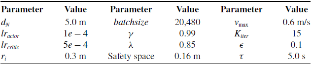
The hyperparameters of the training process and ORCA.

Table I Long description
A table with three rows and three columns listing hyperparameters for a training process and ORCA. The columns are labeled Parameter, Value, Parameter, Value, and Parameter, Value. The table includes the following data: Row 1: Parameter, d N, Value, 5.0 m, Parameter, batchsize, Value, 20,480, Parameter, v max, Value, 0.6 m per s. Row 2: Parameter, l r actor, Value, 1 e - 4, Parameter, gamma, Value, 0.99, Parameter, K iter, Value, 15. Row 3: Parameter, l r critic, Value, 5 e - 4, Parameter, lambda, Value, 0.85, Parameter, epsilon, Value, 0.1. Row 4: Parameter, r i, Value, 0.3 m, Parameter, Safety space, Value, 0.16 m, Parameter, tau, Value, 5.0 s.
Network structure. The number in the block represents the output dimension. The input dimension is determined by the output dimension of the previous layer.

Figure 5 Long description
A diagram of a network structure for deep reinforcement learning combined with ORCA for multi-robot navigation. The diagram shows the flow of data through various layers and components. The input consists of observations related to self and others, processed through fully connected layers (FCL) with 256 units and Tanh activation functions. The processed observations are then fed into a self-attention mechanism, which includes multiple fully connected layers and a mask applied via a softmax function. The output of the self-attention mechanism is combined and further processed through fully connected layers with Tanh activation functions. This processed data is then split into two paths: one leading to an actor network and the other to a critic network. The actor network includes fully connected layers with 256, 128, and 1 units, and Tanh and softmax activation functions, producing the probability distributions for actions. The critic network includes fully connected layers with 256 and 1 units, and Tanh activation functions, producing the value function. The diagram illustrates the integration of deep reinforcement learning with ORCA to enhance navigation and collision avoidance performance in multi-robot scenarios.
Specifically, take robot
 $i$
as an example. Supposing the length of self-state
 ${\boldsymbol{{o}}}_i^{self}$
is
 $L_R$
and each surrounding robot’s state
 ${\boldsymbol{{o}}}_{i,\,j}^{surr}$
is
 $L_{surr}$
. Then,
 ${\boldsymbol{{o}}}_i^{surr}$
is a matrix and the dimension is
 $(M-1) \times (L_{surr})$
, where each dimension corresponds to one robot of surrounding robots. The subtracted
 $1$
corresponds to robot
 $i$
.
 $N$
-dimensions are non-zero vectors, and the remaining
 $M-1-N$
dimensions are
 $\boldsymbol{0}$
-vectors. Before feeding them into the neural network, we concatenate
 ${\boldsymbol{{o}}}_i^{self}$
and each
 ${\boldsymbol{{o}}}_{i,\,j}^{surr}$
to form a matrix with
 $(M-1) \times (L_R+L_{surr})$
. We use a self-attention module to weigh these
 $M-1$
feature vectors into one vector. First, a multi-layer perceptron (MLP) is used to calculate the importance weights of these
 $M-1$
feature vectors to robot
 $i$
’s collision avoidance navigation. Then, we mask the weights corresponding to
 $\boldsymbol{0}$
-vectors to 0 and use a softmax function to ensure the remaining valid weights sum to 1. Then, these importance weights are used to weight these
 $M-1$
feature vectors. When there are no other robots within the
 $d_N$
range of the robot
 $i$
,
 $N=0$
. In this case, the self-attention module cannot provide effective features. So, we additionally use an MLP to sense the self-state
 ${\boldsymbol{{o}}}_i^{self}$
of the robot
 $i$
.
Policy Training Process

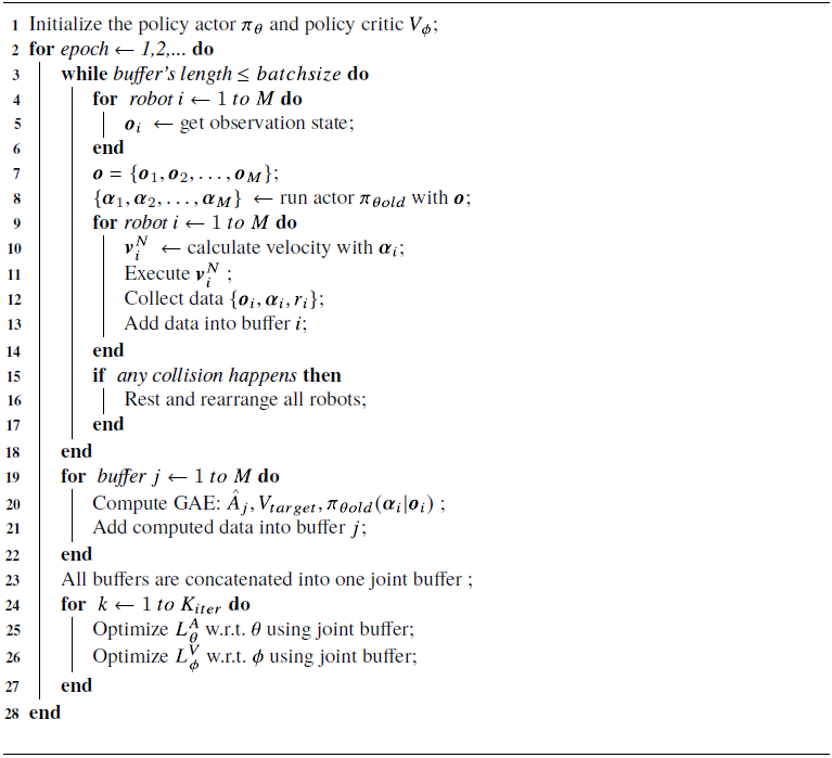
Algorithm 1 Long description
The algorithm outlines the policy training process for robots. It starts by initializing the policy actor and policy critic. The process involves multiple epochs, each consisting of several steps. In each epoch, the algorithm first fills a buffer with data by having each robot get an observation state, run the actor with the current policy, calculate velocity, execute the action, and collect data. If any collision happens, all robots are reset and rearranged. The algorithm then computes the Generalized Advantage Estimation (GAE) for each buffer and adds the computed data into the respective buffer. All buffers are concatenated into one joint buffer. The algorithm then optimizes the policy actor and policy critic using the joint buffer. This process is repeated for a specified number of iterations.
We utilize the actor-critic-based PPO algorithm to train and update our policy. The actor module outputs the action distribution, and the critic module outputs the value function of the observation state. The actor and critic modules have the same network backbone, but the weights (
 $\theta$
and
 $\phi$
) of their backbones are independent. The hyperparameters used for our deployment of PPO and ORCA are aggregated in Table I. The details of the training process are summarized in Algorithm 1. First, our method starts with initializing the actor (
 $\pi _\theta$
) and critic (
 $V_\phi$
) parameters of the orthogonal distribution. To achieve computational and execution efficiency, we calculate actions in a batch form in the neural network, while obtaining the observation state and achieving robot-environment interactions through parallel computing. During the exploration phase, each robot has an independent replay buffer to collect data. When the total number of replay buffers collected by all robots reaches
 $batchsize$
, the exploration is terminated, and network parameters are trained by PPO. The generalized advantage estimator (GAE) is used to estimate the advantage function. The advantage function, value function, and other relevant data of each robot are independently calculated. After the calculation is completed, all buffers are concatenated together in the order of robots to form a joint replay buffer. The joint buffered data is used to construct the surrogate objective loss
 $L^{A}(\theta )$
and value loss
 $L^{V}(\phi )$
as shown in Equations (16) and (17). The optimizer used for parameters update is Adam with eps =
 $10^{-5}$
, learning rate
 $lr_{actor}$
and
 $lr_{critic}$
.
 \begin{equation} L_\theta ^{A} = - \mathbb{E}[H(\pi _\theta (\!\cdot\! |s_t))] - \mathbb{E}\{min[r_t(\theta ),clip(r_t(\theta ),1-\epsilon ,1+\epsilon )]\hat {A}_t\} \end{equation}
where the subscript
 $\theta$
represents the weight parameters of the Actor module,
 $r_t(\theta )$
is the ratio of the probabilities:
 $r_t(\theta ) = \frac {\pi _\theta (a_t|s_t)}{\pi _{\theta _{old}}(a_t|s_t)}$
.
 $\epsilon$
is a hyperparameter used to limit the update magnitude of network parameters.
 $H(\pi _\theta (\!\cdot\! |s_t))$
is the entropy of the action space, which is used in the loss function to encourage DRL to explore the environment.
 $\hat {A}_t$
is the advantage function.
 \begin{equation} L_\phi ^{V} = \mathbb{E}\{max[\Vert V_\phi (s_t) - V_{target}(s_t)\Vert ^2, \Vert clip( V_\phi (s_t), V_{\phi _{old}}(s_t)-\epsilon , V_{\phi _{old}}(s_t)+\epsilon ) - V_{target}(s_t)\Vert ^ 2 ]\} \end{equation}
where the subscript
 $\phi$
represents the weight parameters of the Critic module,
 $V_{target}(s_t)=\mathbb{E}[\sum \limits _{t'=t}^{T} R(s_{t'},\alpha _{t'}) \gamma ^{t'-t} ]$
.
5. Experiments
5.1. Simulation setup
We use the ROS [Reference Quigley, Conley, Gerkey, Faust, Foote, Leibs, Berger, Wheeler and Ng23]-based Gazebo [Reference Koenig and Howard24] as the simulation platform. If any collision occurs among the robots or if the maximum time cost (350 s) is exceeded, the simulation environment will be reset [Reference Chen, Wang, Miao, Feng, Zhou, Wang and Wang25]. Success rate, travel time, and stuck rate are employed to assess the effectiveness of our method and baselines. Success rate is the ratio of all robots in the scene reaching corresponding goals without any collisions. Travel time refers to the cost of time in the simulation when all robots arrive at corresponding goals [Reference Han, Chen, Wang, Zhang, Gao, Hao and Pan1], stuck rate is the ratio of any robot exceeding the maximum time cost when navigating to its goal in one run. Collision rate = 1 – success rate – stuck rate.
We consider two kinds of scenes for comprehensive testing: circle scenes and random scenes. In circle scenes, all robots are randomly and evenly distributed on a circle with a radius of 6 m, and the goal of each robot is set in the opposite direction of the circle. In random scenes, the starting positions of all robots are randomly sampled from a square area with a side length of 12 m and a minimum interval of 1.5 m, and the goals are randomly selected from the starting positions of other robots to increase interactions between them. In all test scenes, all methods are performed for 200 episodes for stable results with various numbers of robots (from 10 to 30). Considering the involvement of nonlearning methods, all learning-based methods are trained only on a circle scene with 10 robots. They are then tested in all scenes directly without any parameter tuning or extra training. The computer we use to train and test methods is a computer with an i7-8700 CPU and a GTX1070 GPU.
To validate the navigation performance of our method, we choose ORCA, VR-ORCA, SARL [Reference Chen, Liu, Kreiss and Alahi22], and RL-RVO as baselines in both circle and random scenes. In addition, two commonly used methods for solving ORCA deadlock problems are also considered as baselines, one is random responsibility (named ORCA-a) and the other is considering observation noise (named ORCA-N). The planning process of ORCA-a is the same as ORCA, except that the reciprocal assumption is not used. For any one of the robots around the target robot, a number uniformly sampled from the interval
 $[0,1]$
is used as the collision avoidance responsibility of the target robot for that robot. However, due to the distributed characteristic of ORCA that does not require communication, the sum of the responsibilities of any two robots sampled for avoiding each other may be less than 1. The planning process of ORCA-N is also the same as ORCA, but noise is added to the position and velocity information of other robots to break the deadlock symmetry, where the position noise is obtained from the uniform distribution
 $[-0.2\,{\rm m}, 0.2\,{\rm m}]$
and the velocity noise is obtained from the uniform distribution
 $[-0.3\,{\rm m/s}, 0.3\,{\rm m/s}]$
. To test whether our simplification of ORCA can break the deadlock situation, we also consider an experimental scheme for an ablation study called ORCA-nearest, which only uses the simplified ORCA proposed in Subsection 4.1 without using DRL.
5.2. Quantitative evaluation
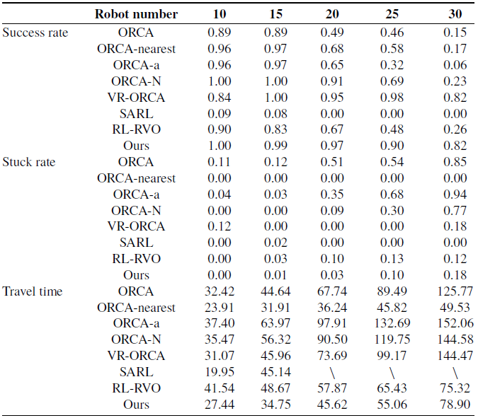
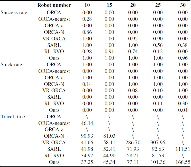
The results in random scenes are summarized in Table II, and the results in circle scenes are summarized in Table III. Among them, ∖” indicates that the method cannot calculate the metric because the success rate is 0.
Generally, as the number of robots increases, the success rate decreases, whereas the travel time increases [Reference Han, Chen, Wang, Zhang, Gao, Hao and Pan1]. The experimental results summarized in two tables also confirm this point. As the number of robots increases, the success rate of all methods decreases to varying degrees. But compared to baselines, our method has the lowest degree of reduction. We only train all methods in a circle scene with 10 robots, but our method still has a relatively high navigation success rate and a low stuck rate in the densest scene with 30 robots.
Experiment results in random scenes.

Table II Long description
The table compares the performance of different robot navigation methods across various metrics and robot numbers. It has 11 rows and 6 columns. The columns are labeled with robot numbers: 10, 15, 20, 25, and 30. The rows are labeled with different navigation methods: ORCA, ORCA-nearest, ORCA-a, ORCA-N, VR-ORCA, SARL, RL-RVO, and Ours. The table is divided into three sections: Success rate, Stuck rate, and Travel time. Each section contains values corresponding to the performance of each method at different robot numbers. Row 1: Success rate, ORCA, 0.89, 0.89, 0.49, 0.46, 0.15. Row 2: Success rate, ORCA-nearest, 0.96, 0.97, 0.68, 0.58, 0.17. Row 3: Success rate, ORCA-a, 0.96, 0.97, 0.65, 0.32, 0.06. Row 4: Success rate, ORCA-N, 1.00, 1.00, 0.91, 0.69, 0.23. Row 5: Success rate, VR-ORCA, 0.84, 1.00, 0.95, 0.98, 0.82. Row 6: Success rate, SARL, 0.09, 0.08, 0.00, 0.00, 0.00. Row 7: Success rate, RL-RVO, 0.90, 0.83, 0.67, 0.48, 0.26. Row 8: Success rate, Ours, 1.00, 0.99, 0.97, 0.90, 0.82. Row 9: Stuck rate, ORCA, 0.11, 0.12, 0.51, 0.54, 0.85. Row 10: Stuck rate, ORCA-nearest, 0.00, 0.00, 0.00, 0.00, 0.00. Row 11: Stuck rate, ORCA-a, 0.04, 0.03, 0.35, 0.68, 0.94. Row 12: Stuck rate, ORCA-N, 0.00, 0.00, 0.09, 0.30, 0.77. Row 13: Stuck rate, VR-ORCA, 0.12, 0.00, 0.00, 0.00, 0.18. Row 14: Stuck rate, SARL, 0.00, 0.02, 0.00, 0.00, 0.00. Row 15: Stuck rate, RL-RVO, 0.00, 0.03, 0.10, 0.13, 0.12. Row 16: Stuck rate, Ours, 0.00, 0.01, 0.03, 0.10, 0.18. Row 17: Travel time, ORCA, 32.42, 44.64, 67.74, 89.49, 125.77. Row 18: Travel time, ORCA-nearest, 23.91, 31.91, 36.24, 45.82, 49.53. Row 19: Travel time, ORCA-a, 37.40, 63.97, 97.91, 132.69, 152.06. Row 20: Travel time, ORCA-N, 35.47, 56.32, 90.50, 119.75, 144.58. Row 21: Travel time, VR-ORCA, 31.07, 45.96, 73.69, 99.17, 144.47. Row 22: Travel time, SARL, 19.95, 45.14, , , . Row 23: Travel time, RL-RVO, 41.54, 48.67, 57.87, 65.43, 75.32. Row 24: Travel time, Ours, 27.44, 34.75, 45.62, 55.06, 78.90.
Experiment results in circle scenes.

Table III Long description
The table presents a comparison of robot performance metrics across different robot numbers, specifically 10, 15, 20, 25, and 30. The table is divided into three main sections: Success rate, Stuck rate, and Travel time, each containing various methods or algorithms. The methods/algorithms listed include ORCA, ORCA-nearest, ORCA-a, ORCA-N, VR-ORCA, SARL, RL-RVO, and Ours. Each method's performance is evaluated across the different robot numbers. Row 1: Success rate, ORCA, 0.00, 0.00, 0.00, 0.00, 0.00. Row 2: Success rate, ORCA-nearest, 0.28, 0.00, 0.00, 0.00, 0.00. Row 3: Success rate, ORCA-a, 0.00, 0.00, 0.00, 0.00, 0.00. Row 4: Success rate, ORCA-N, 0.86, 1.00, 0.00, 0.00, 0.00. Row 5: Success rate, VR-ORCA, 1.00, 1.00, 0.92, 0.90, 0.00. Row 6: Success rate, SARL, 1.00, 1.00, 1.00, 0.56, 0.38. Row 7: Success rate, RL-RVO, 0.98, 0.91, 0.74, 0.12, 0.00. Row 8: Success rate, Ours, 1.00, 1.00, 1.00, 1.00, 0.96. Row 9: Stuck rate, ORCA, 1.00, 1.00, 1.00, 1.00, 1.00. Row 10: Stuck rate, ORCA-nearest, 0.00, 0.00, 0.00, 0.00, 0.00. Row 11: Stuck rate, ORCA-a, 1.00, 1.00, 1.00, 1.00, 1.00. Row 12: Stuck rate, ORCA-N, 0.14, 0.00, 1.00, 1.00, 1.00. Row 13: Stuck rate, VR-ORCA, 0.00, 0.00, 0.08, 0.10, 1.00. Row 14: Stuck rate, SARL, 0.00, 0.00, 0.00, 0.00, 0.00. Row 15: Stuck rate, RL-RVO, 0.00, 0.00, 0.00, 0.11, 0.30. Row 16: Stuck rate, Ours, 0.00, 0.00, 0.00, 0.00, 0.04. Row 17: Travel time, ORCA, , , , , . Row 18: Travel time, ORCA-nearest, 46.14, , , , . Row 19: Travel time, ORCA-a, , , , , . Row 20: Travel time, ORCA-N, 90.93, 81.03, , , . Row 21: Travel time, VR-ORCA, 41.66, 58.11, 286.70, 307.95, . Row 22: Travel time, SARL, 41.98, 52.41, 71.93, 92.63, 111.51. Row 23: Travel time, RL-RVO, 34.97, 44.90, 58.71, 81.53, . Row 24: Travel time, Ours, 37.25, 45.34, 77.11, 101.36, 166.55.
In random scenes where robots are randomly distributed, there are usually only a few cases where robots are symmetrically distributed. Therefore, compared to strictly symmetrical circle scenes, the ORCA method can also navigate robots to their goals. However, as the number of robots increases, the frequency of symmetry in the scene also increases, and the problem of robot deadlocks becomes more frequent, leading to a rapid decline in ORCA’s collision avoidance ability. ORCA-a adopts a random collision avoidance responsibility scheme for multi-robot navigation, but cannot guarantee that the sum of responsibilities for mutual collision avoidance between any two robots is 1, thus cannot guarantee safety constraints. The collision avoidance responsibility not only affects the avoidance ability but also affects the navigation velocity. From the experimental results, it is found that random collision avoidance responsibility actually reduces the movement velocity due to unreasonable responsibility, resulting in longer travel time, and even exceeding the time limit leading to stuck. Adding noise (ORCA-N) to the observation state is more similar to deploying ORCA in real-world environments. Robots need to estimate the states of other robots around them through onboard sensors, thereby introducing observation noise. This type of noise can effectively break the deadlock situation caused by the symmetrical distribution of robots, but the introduction of noise makes ORCA unable to establish accurate collision avoidance constraints and effectively ensure collision avoidance. Among the three original ORCA methods (ORCA, ORCA-a, ORCA-N), ORCA-N is the most effective in solving deadlock problems and navigating successfully. However, when there are more than 20 robots, the frequency of collisions between robots is also the highest. Among all non-learning-based baselines, VR-ORCA calculates collision avoidance responsibility through gradient descent, which is more scientifically reasonable. It achieves the best collision avoidance and navigation ability in random scenes with similar travel time consumption to ORCA and effectively breaks the deadlock situation of robots. Compared to VR-ORCA, the three learning-based methods, including our method, only show significant advantages in travel time. The main issue is that learning-based methods only train in a circle scene containing 10 robots, while reinforcement learning suffers from insufficient generalization, which can affect its performance in testing scenarios different from the training scene. But even though they are affected, our method can achieve collision avoidance and navigation capabilities similar to VR-ORCA.
In circle scenes, the situation of robot deadlocks is denser, and circle scenes can be understood to some extent as the extreme case of random scenes with the same number of robots. In all robot quantity settings, ORCA and ORCA-a are unable to achieve collision avoidance and are completely stuck in deadlock states. In the circle scenes we set up, the goal of each robot is located on the other side of the circle, and all robots gradually approach the center of the circle. The density of robots in the center of the circle is extremely high, and it is difficult to effectively escape the deadlock state by only adjusting collision avoidance responsibilities. The performance of VR-ORCA is also greatly affected. Due to computational efficiency issues, VR-ORCA times out as it cannot escape the deadlock state within the allotted time. Compared to non-learning-based methods, learning-based methods achieve collision avoidance and deadlock-breaking capabilities. SARL and RL-RVO can navigate in this kind of symmetric environment. However, as fully end-to-end reinforcement learning-based methods, their adaptability to environmental changes is not good enough. When the number of robots is different from the training environment, the navigation performance of SARL and RL-RVO decreases significantly in terms of the success rate. Before the number of robots is twice that of the training environment (20), both can still ensure a certain navigation performance. As the number of robots increases from 20 to 30, the navigation performance decreases rapidly, replaced by an increase in collision rate. Our method combines reinforcement learning and ORCA, while exploring the value and direction of collision avoidance responsibility simultaneously. By retaining ORCA’s non-learning-based adaptability to different scenes and combining it with the exploratory ability of reinforcement learning, our method achieves relatively optimal performance.
Based on the experimental results in both random and circular scenarios, all methods can demonstrate varying degrees of collision avoidance and navigation capabilities. Among them, VR-ORCA even achieves relatively better performance in some cases. However, the performance of VR-ORCA is not stable enough in different experiments. VR-ORCA mainly explores how to set collision avoidance responsibilities for each robot more reasonably, without considering changes in avoidance direction. Therefore, in symmetrical experimental scenarios, the performance of VR-ORCA has decreased significantly. In contrast, our method performs stably and has relatively good collision avoidance and navigation performance in both circular and random scenes, without exhibiting particularly poor performance.
5.3. Ablation study
We conduct ablation experiments using only the collision avoidance constraint of ORCA, focusing on the nearest robot introduced in Subsection 4.1, without incorporating the DRL approach discussed in Subsection 4.2. The experimental results are also summarized in Tables II and III.
The experiment results are surprising, as ORCA-nearest performs better than ORCA. But stuck_rate = 0 in ORCA-nearest means that the situation of navigation failure has changed from stuck in the original ORCA to collision in ORCA-nearest. This indicates that retaining only the nearest avoidance constraint does not meet the security guarantee, but it does break the deadlock caused by the symmetry of collision avoidance constraints. Because the stuck_rate is 0. And it has some navigation ability, but its navigation ability is poor when robots are dense. However, in our complete solution, we use DRL to locally adjust the nearest collision avoidance constraint, which not only reduces the occurrence of deadlocks but also effectively ensures the ability of collision avoidance navigation.
When there are multiple robots around, ORCA will generate a collision avoidance constraint for each neighbor robot. These constraints will ultimately generate a collision avoidance velocity space, from which the velocity that can reach the goal the fastest is selected as the robot’s navigation velocity. When multiple robots exhibit a nearly symmetrical distribution, they may get stuck in place, leading to deadlocks. When only one avoidance constraint is used, the symmetrical distribution of constraints will be greatly reduced, effectively solving the deadlock problem. As for collision avoidance navigation, it can be guaranteed by the use of DRL. Simplifying ORCA releases security constraints that can effectively alleviate deadlocks, but cannot guarantee collision avoidance. Therefore, introducing DRL in the simplified ORCA to balance deadlock and collision avoidance issues can effectively avoid deadlocks while ensuring collision avoidance navigation.
When only considering the nearest collision avoidance constraint to plan the velocity, the robot can generate a motion velocity that avoids the nearest robot, but it may cause the robot to approach other robots around it. However, for any robot, the nearest neighbor robot is not fixed. As the robot moves, the nearest neighbor robot keeps changing. If the robot currently avoids the nearest robot, but its movement direction may approach another robot, the robot will move away from the nearest neighbor robot and make the approaching robot the new nearest robot. Afterwards, the robot would avoid this new nearest robot.
Even if there are multiple robots that are closest in space and we only consider one of them, as the robot avoids the nearest one and moves away from it, it will break the situation where multiple robots are closest at the same time, resulting in a situation where there is only one nearest robot. So, in the process of retaining only the nearest collision avoidance constraint navigation, the robot will constantly move, causing the nearest robot to constantly change, and the constraint is constantly changing. For the original ORCA, when multiple nearest robots appear simultaneously, the symmetry of constraints will cause the robots to get stuck, and the position and other information between robots will no longer undergo dynamic motion, resulting in the inability to change collision avoidance constraints and leading to deadlock. When only retaining the nearest collision avoidance constraint, ORCA will be more likely to plan the motion speed of the robot far away from this nearest one, thereby breaking the deadlock problem caused by being at the same distance from multiple robots at the same time.
At present, the generalization ability of DRL itself is relatively limited, but the method used in this manuscript seems to have better generalization ability. Based on our analysis and experimental results, we believe that the improvement in generalization ability is due to the existence of the simplified ORCA. It can be seen that using only simplified ORCA can achieve better navigation capabilities compared to the original ORCA. Although the simplified ORCA does not guarantee sufficient collision avoidance capabilities, it still retains the planning process of ORCA, mainly transforming the deadlock phenomenon of the original ORCA into collisions. So, even if DRL is used to ensure collision avoidance and navigation capabilities, it still has good generalization ability to the environment.
Navigation trajectories of VR-ORCA, SARL, RL-RVO, and ours. The red circle represents the goal position, other colored circles represent robots, and the curve with the same color as the circle represents the robot’s trajectory. The dashed black boxes indicate some unreasonable behaviors, such as occupying extra space to avoid collisions or aggregating (a) VR-ORCA, (b) SARL, (c) RL-RVO, (d) ours.

Figure 6 Long description
The image contains four sets of diagrams labeled (a) VR-ORCA, (b) SARL, (c) RL-RVO, and (d) ours. Each set shows the trajectories of robots avoiding collisions. Panel A: VR-ORCA. This panel contains four diagrams showing the trajectories of robots using the VR-ORCA method. Each diagram has colored circles representing robots and curves indicating their trajectories. The red circle represents the goal position. The dashed black boxes highlight unreasonable behaviors such as occupying extra space to avoid collisions or aggregating. Panel B: SARL. This panel contains four diagrams showing the trajectories of robots using the SARL method. Similar to Panel A, colored circles represent robots, and curves indicate their trajectories. The red circle represents the goal position. Panel C: RL-RVO. This panel contains four diagrams showing the trajectories of robots using the RL-RVO method. Colored circles represent robots, and curves indicate their trajectories. The red circle represents the goal position. The dashed black boxes highlight unreasonable behaviors. Panel D: ours. This panel contains four diagrams showing the trajectories of robots using the method developed by the authors. Colored circles represent robots, and curves indicate their trajectories. The red circle represents the goal position.
5.4. Qualitative analysis
Relaxing the maximum time limit, we obtain the trajectories of VR-ORCA, SARL, RL-RVO, and our method in circle scenes with different numbers of robots as shown in Figure 6.
VR-ORCA achieves asymmetric collision avoidance constraints for symmetrically distributed robots by dynamically adjusting collision avoidance responsibilities, thereby breaking the deadlock situation when all robots approach the center of the scene. However, only adjusting the responsibility has a limited impact on the direction of robot navigation. As the density of robots increases, the phenomenon of robots piling up together becomes increasingly apparent. SARL achieves the simplest and smoothest navigation trajectory, but based on the summary results of quantitative experiments, it can be found that SARL has limited performance in multi-robot collision avoidance navigation. SARL can effectively prevent deadlock problems, but as an end-to-end method, it lacks security constraints similar to ORCA, which cannot guarantee collision avoidance. RL-RVO has similar issues. Although RL-RVO introduces security constraints similar to ORCA by designing reward functions and state spaces based on RVO, RVO also faces deadlock problems in symmetric scenes, resulting in RL-RVO being less effective than SARL. In random scenarios where symmetrical robots are less common, the performance of RL-RVO outperforms SARL when using RVO. Compared to VR-ORCA, the navigation trajectory of the method proposed in this paper is quite similar, as both are improvements made for ORCA and inherit the motion characteristics of ORCA to varying degrees. VR-ORCA becomes more chaotic and time-consuming as the number of robots increases. As indicated by the dashed black boxes in the figure, the aggregation of VR-ORCA is becoming increasingly evident, increasing the pressure on robots to avoid collisions, and some robots need to spend extra time moving to the outside of the scene to avoid collisions. A similar situation also occurs in RL-RVO. While aggregation also occurs in our method, the aggregation area is larger, and the density is relatively lighter, giving robots more space to move and reducing collision avoidance pressure for the robots.
5.5. Real-world collision avoidance
A real-world test: four self-built robots swapping positions.

We conduct a real-world demonstration using four self-built differential-driven robots, as shown in Figure 7(a). The maximum moving speed of each robot is 0.6 m/s, with a radius of 0.3 m, and the number is the robot’s ID for easy differentiation between different robots. In the beginning, the robots are manually placed and distributed symmetrically as much as possible, with each robot’s goal being the starting position of the opposing robot. The starting positions of Robot 1 and Robot 3 are each other’s goals, while the starting positions of Robot 2 and Robot 4 are each other’s goals.
When the robots meet (Figure 7(b)), Robot 1 moves from the right side of its perspective. On this path, Robot 1 may collide with Robot 4, while Robot 4 detours from the left side of Robot 1 to avoid collision with Robot 1. Robot 3 is behind Robot 4, and when Robot 4 moves from the right side of Robot 1, Robot 3 also gradually moves forward behind Robot 4. During this process, Robot 2 almost stops moving to prevent collisions. The goal of Robot 4 is located at the starting position of Robot 2. From Figure 7(a) to (d), Robot 4 moves toward the starting position of Robot 1 as a whole to avoid collisions and moves toward its goal when it is close to the starting position of Robot 1. In Figure 7(d), Robot 4 is no longer in front of Robot 3, and Robot 3 can move smoothly to its goal. When robots 1, 3, and 4 leave the middle position of the area (Figure 7(e)), Robot 2 turns to the right and then moves toward its goal (Figure 7(f)), and finally reaches the goal.
During the entire collision avoidance navigation process, Robot 1 generally navigates from the outside of the area formed by the four robots to the destination. Robot 4 mainly passes through the center of the area to avoid collision with Robot 1 and then turns to the destination. Robot 3 moves behind Robot 4 and proceeds to its destination after Robot 4 yields the way. Meanwhile, Robot 2 remains nearly stationary, waiting for the other three robots to depart before navigating to its destination. The four robots use the same policy to navigate but make different movements according to the different states they face, and finally reach their respective goals without collisions and deadlock.
6. Conclusion
In this paper, we focus on the deadlock problem faced by multiple robots during collision avoidance navigation based on ORCA. We first analyze the causes of the deadlock problem from the perspective of ORCA’s planning principles, then discover that simplifying ORCA’s planning process can break the deadlock situation, and analyze its mechanism of action. By simplifying the planning process, ORCA can control the robot to continuously navigate instead of getting stuck. We then combine the exploration and global optimization capabilities of DRL with simplified ORCA to ensure collision avoidance and navigation performance. Finally, multiple groups of experiments are conducted in circle scenes and random scenes with different numbers of robots. The experimental results verify the effectiveness of the proposed method in breaking the deadlock problem of ORCA and collision avoidance navigation.
The original ORCA can avoid static obstacles by assuming full avoidance responsibility, which we have not yet considered, nor have we considered whether deadlock problems may occur when facing static obstacles. We are currently only considering the situation where there are only robots in the environment. Analyzing whether ORCA has deadlock issues in static scenarios and how to solve this problem is an interesting part to help deploy ORCA in more complex and realistic scenarios.
Supplementary material
The supplementary material for this article can be found at https://doi.org/10.1017/S026357472610349X.
Author contributions
Zhihao Liu helped in conceiving the study and design, acquiring the data, analyzing the data, and drafting the manuscript. Wenjie Na helped in acquiring the data, analyzing the data, and revising the manuscript. Chenpeng Yao helped in conceiving the experiment design and revising the manuscript. Chengju Liu and Qijun Chen helped in providing financial support and hardware equipment. All authors have read and approved the manuscript.
Financial support
This paper is supported by the National Natural Science Foundation of China under Grants (62233013, 62333017, 62403358, 62473295). Shanghai Municipal Science and Technology Major Project (2021SHZDZX0100) and the Fundamental Research Funds for the Central Universities.
Competing interests
The authors declare no conflicts of interest exist.
Ethical approval
Not applicable.


 R0
 R0
 R0