2 Problem formulation

A chemically reactive circular particle (radius  $a$ ) is freely suspended in an unbounded solution (solute diffusivity  $D$ , viscosity  $\unicode[STIX]{x1D702}$ ). The equilibrium solute concentration, at large distances from the particle, is denoted by $c_{\infty }$ . Solute transfer at the particle boundary is modelled using a first-order chemical reaction (Ebbens et al. Reference Ebbens, Tu, Howse and Golestanian2012),

(2.1) $$\begin{eqnarray}\text{solute absorption (per unit area)}=k\times \text{local bulk value of solute concentration},\end{eqnarray}$$

where the rate constant $k$ generally varies along the boundary. Following Sondak et al. (Reference Sondak, Hawley, Heng, Vinsonhaler, Lauga and Thiffeault2016) we restrict the subsequent analysis to situations where $k$ is symmetric about a diameter of the swimmer; self-propulsion accordingly takes place in the form of rigid-body translation in a direction parallel to that symmetry line. Defining ${\mathcal{K}}$ as a characteristic norm of $k$ , relation (2.1) naturally provides the solute-flux scale ${\mathcal{J}}={\mathcal{K}}c_{\infty }$ which, when balanced with diffusion, sets the characteristic scale ${\mathcal{C}}=a{\mathcal{J}}/D$ for the excess solute concentration (relative to $c_{\infty }$ ) around the particle, as generated by interfacial reaction. Note that

(2.2) $$\begin{eqnarray}{\mathcal{C}}/c_{\infty }=\mathit{Da}\end{eqnarray}$$

in which

(2.3) $$\begin{eqnarray}\mathit{Da}=\frac{a{\mathcal{K}}}{D}\end{eqnarray}$$

is the Damköhler number, representing the ratio of diffusive ( $a^{2}/D$ ) to reactive ( $a/{\mathcal{K}}$ ) time scales.

On the macroscale, the short-range interaction between the solute molecules and the particle is manifested by diffusio-osmotic slip (Anderson Reference Anderson1989),

(2.4) $$\begin{eqnarray}\text{slip velocity}=b\times \text{surface gradient of solute concentration}.\end{eqnarray}$$

As in Sondak et al. (Reference Sondak, Hawley, Heng, Vinsonhaler, Lauga and Thiffeault2016) we assume that $b$ is uniform. Note that $b$ is a signed quantity, positive for repulsive interactions and negative for attractive ones. The velocity scale associated with (2.4) is ${\mathcal{U}}=|b|{\mathcal{C}}/a$ . Defining the intrinsic Péclet number $\mathit{Pe}=a\,{\mathcal{U}}/D$ thus gives

(2.5) $$\begin{eqnarray}\mathit{Pe}=\frac{|b|{\mathcal{C}}}{D}.\end{eqnarray}$$

3 Dimensionless formulation

We employ a dimensionless notation where all length variables are normalised by $a$ , as well as a particle-fixed reference system with origin at the particle centre. In that system we work with Cartesian coordinates $(x,y)$ defined such that the $x$ -axis is aligned along the symmetry diameter of the particle. We additionally utilise polar coordinates $(r,\unicode[STIX]{x1D703})$ , with $\unicode[STIX]{x1D703}$ measured in the counterclockwise direction from the $x$ -axis. In what follows we consider the coupled transport-flow problem governing the excess solute concentration $c$ , normalised by ${\mathcal{C}}$ , and fluid velocity $\boldsymbol{u}$ , normalised by ${\mathcal{U}}$ . Our interest is in the velocity $U\hat{\boldsymbol{\imath }}$ ( $\hat{\boldsymbol{\imath }}$ being a unit vector in the $x$ -direction) of the particle relative to the otherwise quiescent liquid; in the particle-fixed reference frame this velocity is manifested as the uniform streaming $-U\hat{\boldsymbol{\imath }}$ at infinity.

The dimensionless solute transport problem is governed by: (i) the advection–diffusion equation,

(3.1) $$\begin{eqnarray}\unicode[STIX]{x1D6FB}^{2}c=\mathit{Pe}\,\boldsymbol{u}\boldsymbol{\cdot }\unicode[STIX]{x1D735}c;\end{eqnarray}$$

(ii) the kinetic condition at the particle boundary,

(3.2) $$\begin{eqnarray}\frac{\unicode[STIX]{x2202}c}{\unicode[STIX]{x2202}r}=(1+\mathit{Da}\,c)f(\unicode[STIX]{x1D703})\quad \text{at}~r=1,\end{eqnarray}$$

where $f=k/{\mathcal{K}}$ is the dimensionless distribution of the rate constant; and (iii) attenuation at large distances,

(3.3) $$\begin{eqnarray}c\rightarrow 0\quad \text{as}~r\rightarrow \infty .\end{eqnarray}$$

Note that condition (3.2) is compatible only with solute consumption, $f\geqslant 0$ .

The flow is governed by: (i) the continuity and Stokes equations (the former tacitly employed in (3.1)); (ii) diffusio-osmotic slip (cf. (2.4))

(3.4) $$\begin{eqnarray}\boldsymbol{u}=M\unicode[STIX]{x1D735}_{s}c\quad \text{at}~r=1,\end{eqnarray}$$

where $M=b/|b|$ and $\unicode[STIX]{x1D735}_{s}$ is the surface-gradient operator; (iii) far-field approach to a uniform stream,

(3.5) $$\begin{eqnarray}\boldsymbol{u}\rightarrow -U\hat{\boldsymbol{\imath }}\quad \text{as}~r\rightarrow \infty ;\end{eqnarray}$$

and (iv) the requirement that the particle is force-free.

The preceding nonlinearly coupled problem provides $U$ as a function of $\mathit{Pe}$ , $\mathit{Da}$ and $M(=\pm 1)$ , as well as $f(\unicode[STIX]{x1D703})$ . In principle, knowledge of $c$ eliminates the need for the detailed calculation of the flow field, since use of the reciprocal theorem (Squires & Bazant Reference Squires and Bazant2006) gives here,

(3.6) $$\begin{eqnarray}U=\frac{M}{2\unicode[STIX]{x03C0}}\int _{-\unicode[STIX]{x03C0}}^{\unicode[STIX]{x03C0}}\left.\frac{\unicode[STIX]{x2202}c}{\unicode[STIX]{x2202}\unicode[STIX]{x1D703}}\right|_{r=1}\sin \unicode[STIX]{x1D703}\,\text{d}\unicode[STIX]{x1D703},\end{eqnarray}$$

which, following integration by parts, provides $U$ as the quadrature

(3.7) $$\begin{eqnarray}U=-\frac{M}{2\unicode[STIX]{x03C0}}\int _{-\unicode[STIX]{x03C0}}^{\unicode[STIX]{x03C0}}c|_{r=1}\cos \unicode[STIX]{x1D703}\,\text{d}\unicode[STIX]{x1D703}.\end{eqnarray}$$

While (3.7) may appear to suggest that $U$ is proportional to $M$ , this conclusion is generally invalidated by the nonlinear action of solute advection. In three dimensions, such a proportionality holds for $\mathit{Pe}=0$ , when solute transport is uncoupled from the flow. Specifically,

(3.8a,b ) $$\begin{eqnarray}c\rightarrow c,\quad \boldsymbol{u}\rightarrow -\boldsymbol{u}\quad \text{under the transformation}~M\rightarrow -M.\end{eqnarray}$$

Since the present transport problem is ill-posed at $\mathit{Pe}=0$ , it is not a priori evident whether the symmetry property (3.8) holds as $\mathit{Pe}\rightarrow 0$ .

In what follows it is convenient to represent $f$ as a Fourier series,

(3.9) $$\begin{eqnarray}f(\unicode[STIX]{x1D703})=\mathop{\sum }_{m=-\infty }^{\infty }F_{m}\text{e}^{\text{i}m\unicode[STIX]{x1D703}},\end{eqnarray}$$

wherein

(3.10) $$\begin{eqnarray}F_{m}=\frac{1}{2\unicode[STIX]{x03C0}}\int _{-\unicode[STIX]{x03C0}}^{\unicode[STIX]{x03C0}}f(\unicode[STIX]{x1D703})\text{e}^{-\text{i}m\unicode[STIX]{x1D703}}\,\text{d}\unicode[STIX]{x1D703}.\end{eqnarray}$$

Since $f$ is real and invariant under the reflection $\unicode[STIX]{x1D703}\rightarrow -\unicode[STIX]{x1D703}$ , $F_{m}$ must also be real, satisfying $F_{-m}=F_{m}$ for all $m$ . Since $f\geqslant 0$ we find from (3.10) that

(3.11) $$\begin{eqnarray}F_{0}>0.\end{eqnarray}$$

(We disregard the trivial case $F_{0}=0$ , where no reaction occurs.) In what follows it is convenient to assume

(3.12) $$\begin{eqnarray}F_{1}>0;\end{eqnarray}$$

since this assumption merely amounts to the choice of the $x$ -axis direction, it can be made with no loss of generality. (We ignore the case $F_{1}=0$ , which is associated with a rather specialised mode of asymmetry.) Assertion (3.12) corresponds to a particle which in some sense is more active at its ‘right’ ( $x>0$ ) side.

4 Small- $\mathit{Pe}$ limit

4.1 Underdeterminacy

Consider now the limit of small Péclet numbers. Since at leading order $c$ is harmonic (see (3.1)), it may be expanded into the following series,

(4.1) $$\begin{eqnarray}c=A\log r+\mathop{\sum }_{m=-\infty }^{\infty }A_{m}\frac{\text{e}^{\text{i}m\unicode[STIX]{x1D703}}}{r^{|m|}},\end{eqnarray}$$

where by symmetry $A_{m}$ are real, satisfying $A_{-m}=A_{m}$ . Once the coefficients of (4.1) are determined, the particle velocity is readily obtained from (3.7):

(4.2) $$\begin{eqnarray}U=-MA_{1}.\end{eqnarray}$$

Substitution of (4.1) into the kinetic condition (3.2) provides the following infinite set of linear equations, valid for all integer $k$ :

(4.3a ) $$\begin{eqnarray}\displaystyle & \displaystyle A\unicode[STIX]{x1D6FF}_{k0}-|2k|A_{2k}=F_{2k}+\mathit{Da}\mathop{\sum }_{l=-\infty }^{\infty }F_{k-l}A_{k+l}, & \displaystyle\end{eqnarray}$$

(4.3b ) $$\begin{eqnarray}\displaystyle & \displaystyle -|2k+1|A_{2k+1}=F_{2k+1}+\mathit{Da}\mathop{\sum }_{l=-\infty }^{\infty }F_{k-l}A_{k+l+1}, & \displaystyle\end{eqnarray}$$

where $\unicode[STIX]{x1D6FF}_{k0}$ denotes the Kronecker delta. It is readily verified that (4.3a ) are invariant under $k\rightarrow -k$ while (4.3b ) are invariant under $k\rightarrow -k-1$ . It is accordingly sufficient to consider only $k\geqslant 0$ .

In the presence of the logarithmic and constant terms, expansion (4.1) does not satisfy the decay condition (3.3). Setting both $A$ and $A_{0}$ to zero is generally incompatible with (4.3). Indeed, for $\mathit{Da}=0$ we find from (4.3a ) with $k=0$ that $A=0$ only if the net flux $F_{0}$ vanishes. One could naïvely propose disregarding the violation of (3.3), justifying it by the observation that the particle velocity is only affected by the values attained by $c$ at $r=1$ (see (3.7)) and is accordingly unaffected by the far-field behaviour. The problem with such a ‘pragmatic’ approach is that the system (4.3) is underdetermined; this underdeterminacy is a genuine one, as different arbitrary choices of the values of $A$ and $A_{0}$ generally result in different values of  $U$ .

4.2 Non-uniformity of the small-Péclet-number limit

It is of course well known (Acrivos & Taylor Reference Acrivos and Taylor1962) that the small-Péclet-number limit is generically singular, in the sense that it becomes non-uniform at large distances. The non-uniformity in the present problem may be traced back to (4.1), which implies that $\unicode[STIX]{x1D735}c$ decays as $1/r$ at large $r$ . With that decay rate we find that the left- and right-hand sides of (3.1) are $O(1/r^{2})$ and $O(\mathit{Pe}/r)$ , respectively; regardless of how small is $\mathit{Pe}$ , advection always enters the leading-order balance at $r=O(1/\mathit{Pe})$ . The preceding expansion (4.1) thus describes the leading-order concentration at an ‘inner’ region, where $r=O(1)$ . It needs to be supplemented by an additional ‘outer’ expansion, valid at $r=O(1/\mathit{Pe})$ . With that approach, the logarithmic ‘divergence’ in (4.1) is acceptable, as it is the outer expansion that needs to satisfy far-field decay. Moreover, since (4.1) holds in the inner region, (4.2) is valid too. The underdeterminacy in (4.3) is now resolved using asymptotic matching between the inner and outer regions.

The outer region is naturally analysed using the stretched coordinates

(4.4) $$\begin{eqnarray}(x^{\prime },y^{\prime })=\mathit{Pe}\,(x,y).\end{eqnarray}$$

Writing $c=c^{\prime }(x^{\prime },y^{\prime };\mathit{Pe})$ and making use of the approach (3.5) to a uniform stream we obtain at leading order (cf. (3.1))

(4.5) $$\begin{eqnarray}\unicode[STIX]{x1D6FB}^{\prime 2}c^{\prime }=-U\frac{\unicode[STIX]{x2202}c^{\prime }}{\unicode[STIX]{x2202}x^{\prime }},\end{eqnarray}$$

wherein $\unicode[STIX]{x1D6FB}^{\prime 2}=\unicode[STIX]{x2202}^{2}/\unicode[STIX]{x2202}x^{\prime 2}+\unicode[STIX]{x2202}^{2}/\unicode[STIX]{x2202}y^{\prime 2}$ is the stretched Laplacian. Substituting $c^{\prime }=\text{e}^{-Ux^{\prime }/2}H$ we find that $H$ satisfies the modified Helmholtz equation, $\unicode[STIX]{x1D6FB}^{\prime 2}H=(U^{2}/4)H$ . The solution of that equation that decays at infinity and is least singular at the origin is a radially symmetric screened source of magnitude $D$ , $(D/2\unicode[STIX]{x03C0})\text{K}_{0}(|U|r^{\prime }/2)$ , in which $r^{\prime }=\mathit{Pe}\,r$ and $\text{K}_{0}$ is a modified Bessel function of the second kind. We therefore obtain

(4.6) $$\begin{eqnarray}c^{\prime }=\frac{D}{2\unicode[STIX]{x03C0}}\text{e}^{-Ux^{\prime }/2}\text{K}_{0}\left(\frac{|U|r^{\prime }}{2}\right).\end{eqnarray}$$

The large-argument behaviour of $\text{K}_{0}$ readily shows that $c^{\prime }$ decays exponentially with $r^{\prime }$ , except in a narrow wake of width $O({r^{\prime }}^{1/2})$ about the negative- $x^{\prime }$ axis where it decays as ${r^{\prime }}^{-1/2}$ .

Using the small-argument behaviour of $\text{K}_{0}$ we find, with an algebraically small error,

(4.7) $$\begin{eqnarray}c^{\prime }\sim \frac{D}{2\unicode[STIX]{x03C0}}\left(-\unicode[STIX]{x1D6FE}-\log \frac{|U|r^{\prime }}{4}\right)\quad \text{as}~r^{\prime }\rightarrow 0,\end{eqnarray}$$

wherein $\unicode[STIX]{x1D6FE}$ is the Euler–Mascheroni constant. Rewriting in terms of the inner variable and performing van-Dyke matching with (4.1) we obtain

(4.8a,b ) $$\begin{eqnarray}A=-\frac{D}{2\unicode[STIX]{x03C0}},\quad A_{0}=\frac{D}{2\unicode[STIX]{x03C0}}\left(\log \frac{4}{|U|\mathit{Pe}}-\unicode[STIX]{x1D6FE}\right),\end{eqnarray}$$

where, following the conventional approach (Hinch Reference Hinch1991), logarithmic terms are considered on par with $O(1)$ terms. Combining (4.8) to eliminate $D$ we obtain using (4.2)

(4.9) $$\begin{eqnarray}A_{0}=-A\left(\log \frac{4}{|A_{1}|\mathit{Pe}}-\unicode[STIX]{x1D6FE}\right),\end{eqnarray}$$

which, together with (4.3) provides the requisite extra condition for determining the coefficients $\{A,A_{0},A_{1},A_{2},\ldots \}$ . While the preceding conditions (4.3) are linear in these coefficients, condition (4.9) is nonlinear in them. This ultimate nonlinearity represents the non-vanishing signature of solute advection. Note that condition (4.9) is compatible with (3.8); since said nonlinearity appears only through that condition, we conclude that the symmetry (3.8) holds at leading order as $\mathit{Pe}\rightarrow 0$ .

With the conventional interpretation of logarithmic terms as being $O(1)$ , the union of (4.3) and (4.9) provides $\{A,A_{0},A_{1},A_{2},\ldots \}$ – and then $U$ by (4.2) – as $O(1)$ quantities in the limit $\mathit{Pe}\rightarrow 0$ . It then follows from (4.9) that the signs of $A_{0}$ and $A$ are opposite: a particle that absorbs solute ( $A>0$ ) results in a decrease of the background solute concentration relative to that at infinity ( $A_{0}<0$ ), and vice versa. While (3.11) appears to suggest that $A$ is positive, it is unclear whether that is indeed the general case.

4.3 The case $\mathit{Da}=0$

The reaction-limited case $\mathit{Da}=0$ represents a situation where diffusion is so fast that the absorption process virtually does not affect the solute concentration (see (2.2)). In that limit the chemical reaction is simply equivalent to the specification of an inward solute-flux distribution of dimensional magnitude ${\mathcal{J}}f(\unicode[STIX]{x1D703})$ . Conditions (4.3) are then independent of $A_{0}$ , and accordingly provide a unique solution for the set $\{A,A_{1},A_{2},\ldots \}$ . In particular we obtain $A=F_{0}$ (as expected) and $A_{1}=-F_{1}$ . While the matching condition (4.9) does provide $A_{0}$ , it may be disregarded if one is only concerned with the swimming velocity, which by (4.2) is given by

(4.10) $$\begin{eqnarray}U=MF_{1}.\end{eqnarray}$$

For $M=1$ , where slip takes place along the solute-concentration gradients, we find using (3.12) that $U>0$ . This is quite obvious: with solute absorption on the right being stronger than on the left, $c$ must be lower on the right to allow for the required diffusive fluxes to supply solute to the absorbing boundary. With the associated slip taking place essentially from right to left, and with the liquid being at rest at infinity, the force-free particle reacts by moving to the right.

4.4 The general case $\mathit{Da}>0$

For $\mathit{Da}>0$ we cannot obtain $U$ in close form. Rather, it is determined by the solution of the infinite algebraic system consisting of (4.3) and (4.9). For illustration we make use of the same Janus configuration considered in Sondak et al. (Reference Sondak, Hawley, Heng, Vinsonhaler, Lauga and Thiffeault2016), namely

(4.11) $$\begin{eqnarray}f(\unicode[STIX]{x1D703})=\left\{\begin{array}{@{}ll@{}}1 & -\unicode[STIX]{x03C0}/2<\unicode[STIX]{x1D703}<\unicode[STIX]{x03C0}/2,\\ 0 & \text{otherwise},\end{array}\right.\end{eqnarray}$$

for which (3.10) gives $F_{2k}=\unicode[STIX]{x1D6FF}_{k,0}/2$ and $F_{2k+1}=(-)^{k}/(2k+1)\unicode[STIX]{x03C0}$ . Given the applicability of the symmetry property (3.8), we have performed the calculation for $M=1$ with no loss of generality. The infinite algebraic system was solved using controlled truncation; for all values of $\mathit{Pe}$ and $\mathit{Da}$ considered we have practically reached convergence with less than $10$ terms in (4.1). Since the differential equations are not solved directly, no need arises for the discontinuous distribution (4.11) to be smoothened (cf. (51) in Sondak et al. Reference Sondak, Hawley, Heng, Vinsonhaler, Lauga and Thiffeault2016).

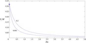
Figure 1 portrays the variation of $U/M$ with $\mathit{Da}$ for two values of $\mathit{Pe}$ . Both curves start with the zero- $\mathit{Da}$ value $F_{1}$ , see (4.10). Evidently, the dependence upon $\mathit{Pe}$ is rather weak. The positive sign of $U$ for $M=1$ is expected with $F_{1}>0$ , although it is unclear whether that it indeed a universal property, valid for all distributions $f(\unicode[STIX]{x1D703})$ .

Figure 1.

$U/M$ as a function of $\mathit{Da}$ for the indicated values of $\mathit{Pe}$ , obtained using the small- $\mathit{Pe}$ approximation. The square represents the corresponding zero- $\mathit{Da}$ value $1/\unicode[STIX]{x03C0}$ .

5 The strong-reaction limit

It was observed in the three-dimensional analysis of phoretic swimmers that the large- $\mathit{Da}$ limit is associated with small fluid velocities (Yariv & Michelin Reference Yariv and Michelin2015). This suggests consideration of that limit in the present 2D problem, where the associated weak advection provides a handle for far-field regularisation.

Given the definition (2.3), the large- $\mathit{Da}$ limit is expected to be realised in situations where $a{\mathcal{K}}$ is large, corresponding to large particles or strong reaction (or both). Now, using the definition of ${\mathcal{C}}$ we find from (2.5) that, in terms of the primitive quantities defining the problem, $\mathit{Pe}=|b|a{\mathcal{K}}c_{\infty }/D^{2}$ – also proportional to $a{\mathcal{K}}$ . This suggests that a limit of interest is

(5.1) $$\begin{eqnarray}\mathit{Da},\mathit{Pe}\rightarrow \infty \quad \text{with}~\mathit{Da}/\mathit{Pe}~\text{fixed}.\end{eqnarray}$$

From the kinetic condition (3.2) it is evident that in the present asymptotic limit $c$ possesses the expansion

(5.2) $$\begin{eqnarray}c=\mathit{Da}^{-1}c^{(1)}+\mathit{Da}^{-2}c^{(2)}+\cdots ,\end{eqnarray}$$

where the leading-order term satisfies $c^{(1)}=-1$ at $r=1$ . We now postulate, subject to a posteriori confirmation, that the distribution $c^{(1)}$ is unaffected by solute advection. Since $c^{(1)}$ is harmonic it must possess the radially symmetric profile

(5.3) $$\begin{eqnarray}c^{(1)}=A\log r-1.\end{eqnarray}$$

As this profile does not contribute any slip, we put forward the asymptotic expansion

(5.4) $$\begin{eqnarray}\boldsymbol{u}=\mathit{Da}^{-2}\boldsymbol{u}^{(2)}+\cdots ,\end{eqnarray}$$

with a similar expansion for the particle velocity $U$ . The relative magnitude of advection in (3.1) is accordingly $\mathit{Pe}/\mathit{Da}^{2}$ . For all $\mathit{Pe}\ll \mathit{Da}^{2}$ , and in particular $\mathit{Pe}$ and $\mathit{Da}$ satisfying (5.1), advection is subdominant. This justifies its neglect in the preceding calculation of $c^{(1)}$ .

At the next asymptotic order we find from (3.2) and (5.3) that $c^{(2)}=A/f(\unicode[STIX]{x1D703})$ at $r=1$ . There is no need to explicitly calculate $c^{(2)}$ , since (3.7) readily provides the leading-order swimmer velocity

(5.5) $$\begin{eqnarray}U^{(2)}=-\frac{MA}{2\unicode[STIX]{x03C0}}\int _{-\unicode[STIX]{x03C0}}^{\unicode[STIX]{x03C0}}\frac{\cos \unicode[STIX]{x1D703}}{f(\unicode[STIX]{x1D703})}\,\text{d}\unicode[STIX]{x1D703}.\end{eqnarray}$$

To obtain $A$ we need to consider the role of advection. With $O(\mathit{Da}^{-2})$ streaming at infinity and with $\unicode[STIX]{x1D735}c$ again decaying as $1/r$ it is evident that in the present problem the dominance of diffusion breaks down at $O(\mathit{Da}^{2}/\mathit{Pe})$ distances from the swimmer, as opposed to the $O(1/\mathit{Pe})$ distances in the small- $\mathit{Pe}$ limit. The outer coordinates are accordingly defined here as $(x^{\prime },y^{\prime })=\mathit{Pe}\,\mathit{Da}^{-2}\,(x,y)$ , cf. (4.4). We then find that the leading-order outer equation (4.5) is still valid provided $U$ is replaced by $U^{(2)}$ . Repeating the asymptotic procedure of § 4 we find using (5.3) that the closure condition (4.9) is replaced here by

(5.6) $$\begin{eqnarray}1=A\left(\log \frac{4\mathit{Da}^{2}}{|U^{(2)}|\mathit{Pe}}-\unicode[STIX]{x1D6FE}\right).\end{eqnarray}$$

Note that $A>0$ regardless of the distribution of $f$ . As in the small- $\mathit{Pe}$ limit, the advection-triggered nonlinear coupling enters only through a closure condition which is compatible with (3.8). We conclude that again $U$ is proportional to  $M$ .

Substitution of (5.6) into (5.5) we obtain a transcendental equation governing  $U^{(2)}$ :

(5.7) $$\begin{eqnarray}U^{(2)}\left(\log \frac{4\mathit{Da}^{2}}{|U^{(2)}|\mathit{Pe}}-\unicode[STIX]{x1D6FE}\right)=-\frac{M}{2\unicode[STIX]{x03C0}}\int _{-\unicode[STIX]{x03C0}}^{\unicode[STIX]{x03C0}}\frac{\cos \unicode[STIX]{x1D703}}{f(\unicode[STIX]{x1D703})}\,\text{d}\unicode[STIX]{x1D703}.\end{eqnarray}$$

For a particle with higher activity on its right side we expect the integral appearing on the right-hand side of (5.7) to be negative. For $M=1$ we then find $U^{(2)}>0$ , as expected. Since (5.7) indicates a slow logarithmic decay of $U^{(2)}$ with $\mathit{Da}^{2}/\mathit{Pe}$ we may obtain an explicit approximation for $U^{(2)}$ by replacing $\log (4\mathit{Da}^{2}/|U^{(2)}|\mathit{Pe})$ with its strict leading-order approximation $\log (\mathit{Da}^{2}/\mathit{Pe})$ , giving

(5.8) $$\begin{eqnarray}U^{(2)}=-\frac{M}{2\unicode[STIX]{x03C0}\log (\mathit{Da}^{2}/\mathit{Pe})}\int _{-\unicode[STIX]{x03C0}}^{\unicode[STIX]{x03C0}}\frac{\cos \unicode[STIX]{x1D703}}{f(\unicode[STIX]{x1D703})}\,\text{d}\unicode[STIX]{x1D703}.\end{eqnarray}$$

Finally, note that the preceding asymptotic analysis remains valid when the limit process (5.1) is relaxed to the mere requirement that $\mathit{Pe}\ll \mathit{Da}^{2}$ as $\mathit{Da}\rightarrow \infty$ .

Unsurprisingly, the large- $\mathit{Da}$ limit is incompatible with absorption-rate distributions wherein $f$ vanishes along a portion of the particle boundary. For illustration purposes we employ here the strictly positive distribution $f=1+\cos \unicode[STIX]{x1D703}/2$ (cf. Yariv & Michelin Reference Yariv and Michelin2015), where the integral appearing on the right-hand side of (5.7) is $(4-8/\sqrt{3})\unicode[STIX]{x03C0}\cong -1.94402$ . 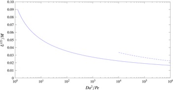The resulting variation of $U^{(2)}/M$ with $\mathit{Da}^{2}/\mathit{Pe}$ is portrayed in figure 2.

Figure 2.

$U^{(2)}/M$ as a function of $\mathit{Da}^{2}/\mathit{Pe}$ . Solid: implicit approximation (5.7). Dashed: explicit approximation (5.8).

6 Relation to Sondak et al. (Reference Sondak, Hawley, Heng, Vinsonhaler, Lauga and Thiffeault2016)

It is useful to relate the present findings to those of Sondak et al. (Reference Sondak, Hawley, Heng, Vinsonhaler, Lauga and Thiffeault2016). Inspection reveals that the quantities $-F$ and $C$ in Sondak et al. (Reference Sondak, Hawley, Heng, Vinsonhaler, Lauga and Thiffeault2016) coincide with the present ${\mathcal{C}}$ and $c_{\infty }$ . Sondak et al. (Reference Sondak, Hawley, Heng, Vinsonhaler, Lauga and Thiffeault2016) choose the two dimensionless groups of the problem as $C/(-F)$ and $(-\unicode[STIX]{x1D707}F)/D$ (their slip coefficient $\unicode[STIX]{x1D707}$ is the same as the present  $b$ ). It is readily seen that these are respectively equal to $1/\mathit{Da}$ (see (2.2)) and $\mathit{Pe}$ (see (2.5)) in the present notation.

In their numerical examples, Sondak et al. (Reference Sondak, Hawley, Heng, Vinsonhaler, Lauga and Thiffeault2016) set $a=D=-F=1$ , whereby their two dimensionless groups become $C$ and $\unicode[STIX]{x1D707}$ . While Sondak et al. (Reference Sondak, Hawley, Heng, Vinsonhaler, Lauga and Thiffeault2016) do not explicitly state how their dimensionless variables are defined, the above setting is equivalent to normalising lengths, concentrations and velocities by $a$ , $-F$ and $D/a$ , respectively. The normalisation of length and concentration variables is accordingly the same as the present one; the different velocity normalisation implies that dimensionless velocities in the present notation are transformed to the notation of Sondak et al. (Reference Sondak, Hawley, Heng, Vinsonhaler, Lauga and Thiffeault2016) via multiplication by $\mathit{Pe}$ (or  $\unicode[STIX]{x1D707}$ ).

With the rate distribution (4.11) being the same as that used by Sondak et al. (Reference Sondak, Hawley, Heng, Vinsonhaler, Lauga and Thiffeault2016) (see (14) there), their results may be directly compared with the present small- $\mathit{Pe}$ approximation. In the absence of solute advection, Sondak et al. (Reference Sondak, Hawley, Heng, Vinsonhaler, Lauga and Thiffeault2016) present the long-time particle speed obtained from a Laplace-transform analysis of the unsteady problem. In the fixed-flux case ( $\mathit{Da}=0$ ) they find (their (27)) an approach to a finite limit which is the same as the present (4.10). In the case of a concentration-limited flux ( $\mathit{Da}>0$ ) they find that the speed attenuates inversely with the logarithm of time; in view of the logarithmic singularity associated with the limit $\mathit{Pe}\rightarrow 0$ (see (4.9)) such an attenuation is indeed expected.

Sondak et al. (Reference Sondak, Hawley, Heng, Vinsonhaler, Lauga and Thiffeault2016) also present numerical results which describe the steady-state transport in the presence of advection. It appears that the only illustration in Sondak et al. (Reference Sondak, Hawley, Heng, Vinsonhaler, Lauga and Thiffeault2016) which is relevant to the present small- $\mathit{Pe}$ analysis appears in their figure 6, where, in the present notation, the variation of $\mathit{Pe}\,U$ is portrayed as a function of $1/\mathit{Da}$ for various values of $\mathit{Pe}$ , the smallest one being $\mathit{Pe}=0.2$ . The trend observed in that figure, where the particle velocity decreases with increasing $\mathit{Da}$ , is in agreement with the present figure 1. The smallest value of $\mathit{Da}$ in figure 6 of Sondak et al. (Reference Sondak, Hawley, Heng, Vinsonhaler, Lauga and Thiffeault2016) is 0.1; the corresponding value of $\mathit{Pe}\,U$ may be visually interpreted from that figure as roughly 0.05, implying $U$ which is approximately 0.25. For these values of $\mathit{Pe}$ and $\mathit{Da}$ , our asymptotic approximation gives $U=0.2567$ (see figure 1).

In their figure 4, Sondak et al. (Reference Sondak, Hawley, Heng, Vinsonhaler, Lauga and Thiffeault2016) show the time evolution of the swimmer velocity for $\mathit{Pe}=50$ and various of values $\mathit{Da}$ , the largest being 10. These values marginally fit into the limit process (5.1). Unfortunately, the use in Sondak et al. (Reference Sondak, Hawley, Heng, Vinsonhaler, Lauga and Thiffeault2016) of the Janus-type distribution (4.11) stands in the way of any meaningful comparison between their numerical results and the present large- $\mathit{Da}$ asymptotic approximation, which breaks down for such distributions.

7 Concluding remarks

In recent years it has been realised that solute advection results in a wide range of non-trivial autophoretic phenomena. These include spontaneous motion of isotropic particles (Michelin, Lauga & Bartolo Reference Michelin, Lauga and Bartolo2013), nonlinear modification of swimming speeds at finite (Michelin & Lauga Reference Michelin and Lauga2014) and large (Yariv & Michelin Reference Yariv and Michelin2015) Péclet numbers, and the instigation of phoretic motion by externally imposed flows (Yariv & Kaynan Reference Yariv and Kaynan2017). The present contribution, inspired by the recent work of Sondak et al. (Reference Sondak, Hawley, Heng, Vinsonhaler, Lauga and Thiffeault2016), has focused upon the critical role played by advection in regularising the ill-posed 2D problem. The singular dependence of the swimming velocity upon the Péclet number has been illuminated in the context of two weak-advection limits. The first is that of small Péclet numbers; the second is that where both the Péclet and Damköhler numbers are large and comparable.

In motivating their analysis, Sondak et al. (Reference Sondak, Hawley, Heng, Vinsonhaler, Lauga and Thiffeault2016) refer to the motion of disk-like swimmers in either Hele-Shaw cells or thin films. While an effective 2D description may be applicable to the Hele-Shaw geometry, it is evident that the sidewall drag on the swimmer prevents a direct use of results obtained for the literal 2D problem formulation. On the other hand, the problem of swimming in a thin film which is immersed in a low-viscosity fluid appears closely related to the idealised 2D model, since the vanishing of shear stresses across the bounding sheets is compatible with a 2D flow.

This thin-film problem is somewhat related to the work of Saffman & Delbrück (Reference Saffman and Delbrück1975) on the Brownian motion of cylindrical particles in membranes. The motivation for that classical work had to do with the anomaly of the Stokes–Einstein relation in two dimensions, where the translational mobility does not exist – the so-called Stokes paradox. The standard regularisation of this paradox, which involves incorporation of inertia at the Oseen region, results in a force-dependent mobility; as such, it is inapplicable to Einstein’s theory. Saffman & Delbrück (Reference Saffman and Delbrück1975) suggested three rational ways to calculate the diffusion coefficients of the cylinders: (i) consideration of a finite-size membrane; (ii) accounting for the viscosity of the suspending fluid; and (iii) direct calculation of the mean-squared displacement from the Langevin equation using the unsteady drag expression.

In the problem of phoretic swimmers the anomaly has to do with solute transport, rather than with the hydrodynamics; furthermore, there is no fundamental objection to the use of small-advection regularisation, as carried out in the present contribution. Nonetheless, proper adaptation of the various approaches of Saffman & Delbrück (Reference Saffman and Delbrück1975) may provide additional insight. Direction (iii) of Saffman & Delbrück (Reference Saffman and Delbrück1975) brings to mind the unsteady approach used by Sondak et al. (Reference Sondak, Hawley, Heng, Vinsonhaler, Lauga and Thiffeault2016). Following direction (ii) of Saffman & Delbrück (Reference Saffman and Delbrück1975) one could envision a mass transfer model which allows for solute diffusion across the thin-film boundaries. It is plausible that such a model would also regularise the transport problem, thereby providing an alternative to the routes taken in Sondak et al. (Reference Sondak, Hawley, Heng, Vinsonhaler, Lauga and Thiffeault2016) and the present contribution.