

1 Introduction
This paper estimates the risks of financial distress in UK universities, and uses these estimates to examine the basis of the annual levies paid to the Pension Protection Fund (PPF) by the Universities Superannuation Scheme (USS), The UK's PPF, modelled on the US's Pension Fund Guarantee Corporation, was established in 2005 and pays compensation to members of occupational defined benefit pension schemes when their employer becomes insolvent and is unable to honour its pension commitments. The PPF operates like an insurance company where members of solvent schemes pay an annual levy in exchange for future compensation in the event of insolvency. Like any insurance product, critical questions relate to whether the insurance premium is fairly priced, and the degree of cross-subsidy between the insured heterogeneous institutions.
Pension schemes protected by the PPF can have more than one employer and in these cases are referred to as multi-employer schemes. Under the rules of the PPF, a multi-employer scheme can either participate on the basis of individual employer schemes insured by the PPF (segmented arrangement) or participate in a self-insured pool, where the PPF will not step in until the last participating member of the pool – the last employer – becomes insolvent (last-man-standing arrangement). Under a last-man-standing (LMS) arrangement, each scheme still has to pay PPF the levies, and has to support scheme members whose employers have became insolvent until the last employer falls into bankruptcy. The PPF charges risk-based levies to solvent schemes, and, in the case of multi-employer schemes, these levies depend on the correlations between the constituent employers, and whether the arrangements are LMS or segmented.
This paper investigates the empirical trade-off between the two PPF participating arrangements for multi-employer pension schemes, namely LMS and segmented levies, using a sample dataset from participating higher education (HE) institutions in the Universities Superannuation Scheme (USS) Ltd. USS Ltd is the UK's fourth largest occupational pension scheme and is an example of a multi-employer scheme, covering 391 universities and related institutions in the UK, with 239,144 members and assets of £30.138 billion.Footnote 1 The USS scheme had a deficit of £6.568 billion at the full actuarial valuation on 31 March 2005, and, therefore, a study of the issues surrounding the choice by USS Ltd, as a multi-employer pension scheme, of the basis for its participation in the UK's Pension Protection Fund is timely.
To assess the insolvency risk of USS participating institutions, the paper introduces a modification of the traditional bankruptcy prediction models, applicable to not-for-profit organizations such as universities. It may seem surprising that universities face insolvency risk, but we note that USS is required to pay into the PPF fund on the basis of the sponsoring employer's risk profile. Under the provisions of the Pensions Act 2004, sponsoring employers must pay into the PPF, and the levy must be partly risk-based, reflecting the sponsoring employer's risk of insolvency. There are two main categories of insolvency: stock-based insolvency, which occurs when the value of a firm's assets is less than its liabilities, and flow-based insolvency, which occurs when firms' cash inflows are insufficient to cover contractually required outflows.Footnote 2 Due to the unlikely event that the assets of an HE institute fall below its liabilities, it is the flow-based definition of insolvency that we will focus on in relation to HE institutions. Even with this restricted definition, it may seem unlikely that a UK HE institution will go bankrupt – although a small number of institutions have been threatened with a bankruptcy process in the past few years.Footnote 3 In discussing the financial problems at University College Cardiff in 1987, Smith and Cunningham (Reference Smith, Cunningham, Warner and Palfeyman2003) report on the hands-on role of the University Grants Commission (UGC), ‘The direct intervention of the UGC broke all the conventions that had been established to separate universities from government influence … From this time on government … would play a much more interventionist role’ (page 29). An implication of this policy change is that in a future changed political climate, the funding councils may reverse this policy and re-adopt a less interventionist role. Indeed McClintock and Ritchie (Reference McClintock, Ritchie, Warner and Palfeyman2003) note that the funding councils refused to intervene in the financial crisis at Lancaster University in 1995–97, ‘They had been told that they would get no help from the Funding Council … and the University should make its own way’ (Lancaster's Vice-Chancellor, quoted in McClintock and Ritchie, Reference McClintock, Ritchie, Warner and Palfeyman2003: 40), and ‘The HEFCE was unwilling to do other than reschedule monthly payments of the recurrent grant’ (ibid.: 40).
Rather than investigate bankruptcy probabilities, instead we look at the probability that an HE institution encounters financial distress, which could lead to ‘potential’ insolvency of the institution. The term ‘financial distress’ refers to ‘a situation where a firm's operating cash flows are not sufficient to satisfy current obligations and the firm is forced to take corrective action’.Footnote 4 Our paper is informed by the empirical findings of Kraatz and Zajac (Reference Kraatz and Zajac1996) that distressed HE institutions are likely to be those undergoing a restructuring, and abnormal Funding Council (FC) grants are taken as an indicator of such restructuring. The Ohlson (Reference Ohlson1980) logit model is used to predict the probability of these abnormal FC grants, and this prediction model is then used to assess the insolvency risks for USS and its participating institutions. Together with other data, such as the pension funding ratio, the levies under LSM and segmentation will be calculated and compared.
We find that financially distressed institutions are smaller in size, with higher leverage ratio and lower earnings, which is consistent with the conventional results of bankruptcy prediction literature. As a robustness check for the prediction power of our model, we compare the institutions identified as being in financial distress with the list of HE institutions at risk of financial failure recently disclosed by the Education Guardian (10 July 2007). We find that over two-thirds of the universities from the Guardian list can be retrieved by our model. We use information provided by USS on its levies to the PPF to calculate the implied probabilities of insolvency of USS institutions and compare these implied probabilities with the simulated insolvency probability using our empirical specifications, and we estimate whether USS levies are fairly priced. Our estimates suggest that in 2006/07, USS member institutions appeared to be paying less than the fair risk-based levy. However, this is because during the initial phase of the PPF, the risk-based levies were much lower as a proportion of the total levy than the intended steady-state values. The implication is that if USS had paid the same total levy, but where the risk-based component was four-fifths of the total (the intended long-run solution), then USS would have been paying substantially more than its fair risk-based levy. By looking at the distribution of risk-based levies for individual institutions under a segmented arrangement with the PPF, we find an asymmetric distribution skewing towards lower values, providing evidence of cross-subsidy under the current LMS arrangements from institutions with better financial conditions to potentially financially distressed institutions.
The paper is organized as follows: Section 2 discusses current bankruptcy prediction models and defines the proxies for financial distress in HE institutions, and a modified prediction model is introduced. Section 3 provides descriptive statistics of the data for the variables used in the analysis. Section 4 presents the empirical results and evaluates the prediction performance of the model. Section 5 gives a detailed discussion of the PPF and the calculation of risk-based levies and Section 6 uses the empirical results to estimate different levies under alternative participation rules and suggests appropriate USS PPF levies. Section 7 presents robustness checks for the model using different measures of financial distress within HE institutions. Section 8 concludes the paper.
2 Financial distress and bankruptcy prediction models
Altman's (Reference Altman1968) multivariate discriminant analysis (MDA) of bankruptcy prediction provides an early statistical analysis of financial ratios as important indicators of corporate failure. Instead of the MDA model, we follow Ohlson (Reference Ohlson1980) who developed a logit bankruptcy model to avoid the problems associated with the MDA analysis. Logit and probit models state that the probability of a firm failing within some pre-specified time period is a function of the product of a vector of predictors and a vector of unknown parameters. Depending on the functional form of the dependent variables, it is called a probit (normal distribution) or logit (logistic cumulative distribution) model. For an event Y to occur (Y=1), the logit model has the form

where X is a vector of explanatory variables. The logit model is estimated by maximizing the log-likelihood function

In bankruptcy prediction models, the predictors capture the firm's characteristics such as size, profitability, leverage, and cashflow. Ohlson (Reference Ohlson1980) uses firm's characteristics, such as size, and financial ratios, such as total liabilities/total assets (reflecting leverage), working capital/total assets (reflecting liquidity), current liabilities/current assets, and net income/total assets (performance measurement). He finds greater prediction powers using a logit model than the z-score model by Altman (Reference Altman1968) and Taffler (Reference Taffler1982). Using UK data, Lennox (Reference Lennox1999) finds superior predicting power of well-specified non-linear probit and logit models over MDA and linear probit and logit models, and finds that compared to non-failing companies, failing companies are typically small, have poor cashflow and profitability, and are highly leveraged.
We apply the probit/logit model to evaluate the insolvency risks for USS participating institutes. Unlike publicly traded firms in the private sector, government support makes it almost impossible for a UK HE institution to go bankrupt and, therefore, an appropriate proxy for financial distress needs to be chosen to identify the insolvency risk. Kraatz and Zajac (Reference Kraatz and Zajac1996) argue that organizations facing financial distress are more likely to recognize the need for strategic change/restructuring. Therefore, they use measures that capture organizational restructuring as the proxy for financial distress and find that institutions undergoing restructuring have lower income, higher debt, and lower reputations, which are variables related to specific situations of financial distress. In our paper, the choice of predictor for financial distress is related to Kraatz and Zajac (Reference Kraatz and Zajac1996): we identify ‘unanticipated payments’ from the funding councils to HE institutions as the indicator of financial distress.
HE institutions in the UK attract income from a variety of sources. These include tuition fees, funding council (FC) grants, research grants and contracts, endowments and investment income, and other income. Funding council grants provide the largest proportion at around 38%.Footnote 5 The funding council grants fall into four main categories: funding for teaching, funding for research, special funding, and capital funding. The teaching and research grants are allocated by formula, with the former mainly related to student numbers, which institutions are required to deliver in return for the funding, and the latter related to the research quality, staff numbers, and the most recent RAE (Research Assessment Exercise) performance of an institution. The special funding is attributed to institutions for specific purposes such as learning and teaching strategies, widening participation, regional collaboration, and closer links between HE and business and the wider community. The capital funding is used to help build the infrastructure for HE institutions.
There are three FCs in the UK, namely the Higher Education Funding Council for England (HEFCE) and Wales (HEFCW), and Scottish Funding Council (SFC, formerly Scottish Higher Education Funding Council – SHEFC).Footnote 6 These funding councils publish in their annual reports the expected allocation for the following year of the largest four categories of grants: teaching and research grants, special funding and capital funding. As these four kinds of funding take up the majority of funding council grants for most HE institutions, the sum of the funding from those four categories can be regarded as the best estimate for the expected funding council grants in the following year.
The Higher Education Statistics Agency (HESA) also publishes annual data on the realized funding council grants for each HE institution. The difference between the predicted funding council grant and HESA's actual grant is the ‘unanticipated payments’, and we take these unanticipated payments as evidence of financial distress. This is because we would expect that, for financially solvent institutions, the actual grants received would be similar to what was expected. Indeed the Chief Executive of HEFCE, in evidence to the Parliamentary Select Committee on Education and Skills on 19 October 2005, explained that ‘Part of the raison d'Etre of the Funding Council, and always has been, is to intervene at an early stage before institutions get themselves into so much trouble that they fold’ (Answer to Q57). We define the difference between the realized (HESA) and the anticipated funding council grants (FC) as

where subscript it indicates the value for institution i in year t. ΔGRANTS it is the difference between the actual funding council grants and its predicted value, and can be either positive or negative. A positive ΔGRANTS it value means there were some grants paid in addition to those predicted from the four main categories of FC grants. A negative ΔGRANTS it implies that the realized HESA grants were less than the predicted funding council grants. In both cases large forecast errors on the absolute values of this difference is taken to reflect institutional financial distress. For large positive values of ΔGRANTS it, the institution is being given additional unanticipated funding, and could reflect the need for cash flows from the funding councils. For example, the annual HEFCE report on how much money it would distribute to Universities in 2004–05 revealed that 13 institutions facing serious cuts would receive ‘safety-net’ grants totalling £3.7 million. In particular, Cranfield University whose research money had been reduced by 9.3% per year following poor RAE2001 performance, had received emergency funding of £3 million in the preceding year.Footnote 7 On the other hand, large negative unanticipated payments mean that institutions received less monies than they were expecting, possibly due to a decline in the drivers in the forecasting model, such as a decline in student numbers. For example in 1998–99, HEFCE withheld funds from the University of East London, when it discovered discrepancies in student numbers after a data audit. Similarly, in 2002 HEFCE withdrew £6.2 million of its grant from London South Bank University following under-recruitment.Footnote 8
As larger institutions are likely to receive higher grants from the funding councils and have a large absolute value of ΔGRANTS it, we scale this variable by the total assets of an institution (SIZE it). We then define a dummy variable ABNML indicating whether an institution receives significant ‘unanticipated ad hoc payments’ as

The value of the dummy variable ABNML reflects the size of the forecast error in equation (3) and identifies the distribution of these ‘unanticipated payments’ from a reasonable range, i.e. the mean of ΔGRANTS it/SIZE it.Footnote 9 We will see that the distribution of ΔGRANTS it/SIZE it is highly leptokurtic, and justifies the use a dummy variable for these abnormal grants. A further advantage for choosing this unanticipated change in funding as the predictor for financial distress is that it avoids using the leverage ratio or earnings – two fundamental variables that may be used to define financial distress, but also appear to be equally important in traditional bankruptcy prediction models – as the predictor.Footnote 10
Our measure of financial distress may be compared with another definition identified by the Funding Councils. Using information obtained from HEFCE under the Freedom of Information Act, Education Guardian (10 July 2007) identified 46 universities on the HEFCE's list of institutions ‘at risk’ of financial failure between 1998 and 2003. In effect, our empirical model is attempting to replicate the HEFCE criteria using publicly available information. In Section 5 below, we compare our list of institutions in financial distress with the Guardian list.Footnote 11
The financial distress prediction model in this paper adapts the empirical models of Ohlson (Reference Ohlson1980) and Lennox (Reference Lennox1999). Explanatory variables include: the size of the institution (LNSIZE) (calculated as the logarithm of total assets), working capital/total asset ratio (WCTA), total liabilities/total assets ratio (TLTA), current liabilities/current asset ratio (CLCA), total long-term liabilities/total assets ratio (LLTA), earnings before interest and taxes/total asset ratio (EBITTA), and variables representing the growth path of earnings (NEGTWO and GROW). The estimated model is

where NEGTWO is set to equal to 1 if EBIT is negative for the last two years and 0 otherwise and

is an equation used by McKibben (Reference McKibben1972) to measure the change in earnings. The subscripts t and t−1 imply that the data from the previous year are used to predict the EBIT value in the current financial year. The discussion above and the previous work on financial distress suggest that size and working capital should be positively related to the financial health of an institution. Earnings patterns and earnings growth both relate to the flow-based aspect of financial distress and institutions with higher earnings and earnings growth tend to be safer and vice versa. The leverage ratio measures the ability of an institution to pay back its debt and should be lower the better is the financial solvency of the institution. To summarize, α1, α2, α4, and α6 are expected to be negative and α3 and α5 should be positive.
3 Data and descriptive statistics
The data for HE institutions are obtained from Higher Education Finance Plus dataset provided by Higher Education Statistics Agency (HESA). This dataset contains the full financial statistics returned from annual accounts for UK HE institutions. Data include detailed income and expenditure analysis and balance sheet information. They also contain finance profile ratios in the recent editions. The data used in this paper cover HE Finance Plus data from 2001 to 2005. All the variables used are book values. EBIT is defined using the HESA terminology as the ‘deficit/surplus on continuing operations after depreciation of fixed assets at valuation and before exceptional items, tax and minority interest’, and is equal to the difference between total income and total expenditure on the consolidated income and expenditure statement. For HE institutions in England, Scotland, and Wales the data for funding allocation are published annually by HEFCE, SFC, and HEFCW, respectively. Since HE institutions in Northern Ireland are funded by DELNI jointly with other institutions,Footnote 12 four Irish institutions in the HESA dataset are not included in the analysis.
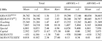
Panel A of Table 1 shows the distribution of funding council grants for the sample institutions from the two sources: HESA HE Finance Plus dataset (GRANTS HESA) and the grants allocation data from the funding councils (Teaching, Research, Special and Capital), for three groups, namely the whole sample, and the two sub-samples of institutions with and without the large ‘unanticipated payments’, as calculated from equation (4). It can be seen that grants for teaching and research take up 70% of the FC grants for the whole sample, and institutions identified as at risk (ABNML=1) have a higher percentage of special funding. Further the realized grants for the ABNML=1 sample is half as large as the not-at-risk sample, which is consistent with the at-risk sample, being predominantly smaller institutions. The distribution of the normalized ΔGRANTS is highly leptokurtic, which provides an additional motivation for defining ABNML=1 where the absolute value of the deviations of ΔGRANTS/SIZE from its mean represents an abnormal financial state. Note that the special funding for distressed and non-distressed institutions are similar in absolute values, implying that distressed institutions receive more funding for specific purposes after taking into account their relatively smaller size. By construction, the elements in the row ΔGRANTS, shows that institutions identified as being in financial distress have a much higher standard deviation of these ‘unanticipated payments’ than those institutions not in financial distress.
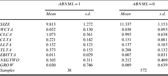
This table reports the mean, standard deviations, skewnes, and kurtosis for the variables of the logit model defined in equation (5) using the HESA HE Finance Plus dataset of 158 HE institutes from 2002 to 2005. Panel A reports the descriptive statistics for funding council grants and Panel B for the regression variables. GRANTS HESA is the total FC grants disclosed by the HESA HE Finance Plus. Teaching, Research, Special and Capital are the teaching, research, special and capital grants disclosed by individual FCs. ΔGRANTS is defined as in equation (3). ABNML is defined in equation (4). SIZE is the total book assets (TA). WCTA is the ratio of working capital to total assets. CLCA is current liabilities divided by current assets (CA). CLTA is current liabilities divided by total assets. LLTA is long-term liabilities divided by total assets. TLTA is the ratio of total liabilities (CL+LL) to total assets. EBITTA is the ratio of EBIT (earnings before interest and taxes) to total assets. NEGTWO is set to be equal to 1 if EBIT is negative for the last two years and 0 otherwise. GROW is the McKibben (Reference McKibben1972) growth ratio defined in equation (6).
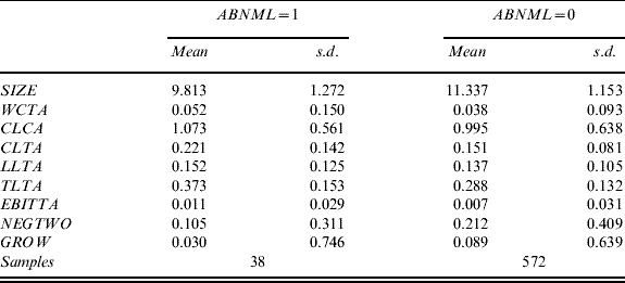
Panel B of Table 1 reports the descriptive statistics for the input variables for two groups of institutions: those with and without significant abnormal funding council grants. In total there are 38 institutions identified as having abnormal FC grants for the five sample years 2001–2005 and 572 institutions without abnormal grants. So around 6% of institutions are receiving abnormal grants and are regarded therefore as being in financial distress or ‘at-risk’. Institutions with abnormal grants are significantly smaller sizes than the rest of the sample (this is equivalent to over £65 million in absolute value), which means smaller institutions are relatively vulnerable to financial distress. However, since the difference between FC grants from the two data sources are weighted by total assets when calculating ABNML, it is possible that smaller institutions are more likely to have larger ratios and consequently be identified as having abnormal grants. Therefore, the size effect is taken into account in the empirical analysis.
Institutions with higher working capital and, therefore, a higher current ratio should be less likely to encounter financial distress; however, the results in the descriptive statistics do not suggest this behaviour. The mean of the inverse of the current ratio (CLCA) for institutions with abnormal grants is 1.1 – just slightly greater than that of those identified as safer institutions. The ratio of working capital to total assets (WCTA) is 5.2% for institutions with abnormal grants, which is higher than 3.8% for those without abnormal grants. This is possibly because cash is less important in the HE sector than industrial sectors. As for variables related to cash generating abilities, again there are some surprising results. For example, the earning/asset ratio (EBITTA) for ‘distressed’ institutions is 1.1%, which is 0.4% higher than those identified as ‘safe’. However on reflection, from the definition of the ABNML variable, this result is not that surprising, since institutions with ABNML=1 value tend to have smaller sizes. Actually, when looking at EBIT alone, the finding is reversed – the mean figure is £46,000 for distressed institutions and over £800,000 for non-distressed ones. The mean earnings growth (GROW) for institutions with higher abnormal grants is 3%, whilst it is 9% for the rest of the institutions, indicating that it is indeed the institutions with lower earnings growth that experience higher unanticipated payments.
The leverage ratios support the stock-based view of financial distress. The ratio of total debt to total assets is 0.37 for institutions with ABNML=1 and 0.29 for those with ABNML=0. This finding suggests that institutions with larger unanticipated abnormal grants are more financially constrained than other institutions, and this evidence is further supported by decomposing total liabilities into current and long-term liabilities. The liability that differentiates the two groups more notably is the current liability (CLTA), which is 0.22 for institutions with abnormal grants, 0.7 higher than their counterparts. This implies that institutions with higher abnormal grants are more financially distressed and thus have lower liquidity than financially stable institutions.
We might argue that by including non-USS institutions within the HESA dataset in the financial distress regressions, the results might be biased due to the unobserved correlations between pensions and cash flows or corporate expenditures.Footnote 13 Here we assume that there is no cross-correlation between the explanatory variables and pensions, and including the maximum number of institutions ensures the most precise estimates that best fit the HE sector. As a robustness check, we included only USS participating institutions in our regressions, but this did not alter the results significantly.Footnote 14
4 Empirical results for the prediction model
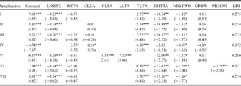
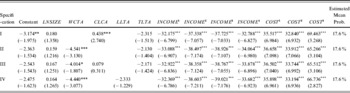
Table 2 reports the prediction results for the logit model in equation (5) under seven different specifications. Unlike the univariate analysis in the descriptive statistics, the logit regression shows that the main results have the same patterns and predicted signs as the Ohlson (Reference Ohlson1980) logit model, and we take this as evidence that our model and dependent variable used are a valid representation of financial distress within the HE sector.
Prediction results for the logit model
The table represents the results for the logit regression described in equation (5) with dependent variable as Pr (ABNML t=1|X), where X is the set of explanatory variables. ABNML is defined as in equation (4) and is the measure of financial distress. LNSIZE is the log of total book assets (TA). WCTA is the ratio of working capital to total assets. CLCA is current liabilities divided by current assets (CA). CLTA is current liabilities divided by total assets. LLTA is long-term liabilities divided by total assets. TLTA is the ratio of total liabilities (CL+LL) to total assets. EBITTA is the ratio of EBIT (earnings before interest and taxes) to total assets. NEGTWO is set to be equal to 1 if EBIT is negative for the last two years and 0 otherwise. GROW is the McKibben (Reference McKibben1972) growth ratio defined in equation (6). Specification (I) is the basic model as in Ohlson (Reference Ohlson1980). Specification (III) adds current liabilities in the regression and specification (II) excludes working capital from specification (II). Specification (IV) removes the size variable to check whether there exists any size effect. Specification (V) splits TLTA into CLTA and TLTL to look at the effects of different liabilities. Specification VI adds in a pre-1992 university dummy. Specification (VII) is the one used in the simulation in Section 7. Robust t-statistics are reported in the parenthesis and *, **, *** stand for 10%, 5%, and 1% significance levels, respectively.

In specification I, the coefficient on the size variable (LNSIZE) is −1.25 and is significant at 99% confidence level. This result holds across all the alternative specifications of the model, and suggests that smaller institutions are more likely to be in financial distress. The leverage ratio (TLTA) measures how much the institution's assets decline in value (market value of assets plus debt) before the liabilities exceed the assets and the institution becomes insolvent. This is a commonly used predictor for bankruptcy because of its direct link to the stock-based definition of financial distress. In specification I, the coefficient estimate for the leverage ratio is 5.73 and is significant at 99% confidence level. The results hold for specifications II, III, and IV, where the coefficient estimates are all positive and very significant. Specification V decomposes total liabilities into current liabilities (CLTA) and long-term liabilities (LLTA). The coefficient estimate for CLTA is 4.38 and 7.32 for LLTA, which are both significant at 99% confidence level, but are not significantly different from each other.
The variable EBITTA (EBIT divided by total assets) captures earnings power of the assets and measures the true productivity of the institution's assets net of any tax or leverage effects. The regression result is as expected: for all specifications (except specification IV), with the coefficient estimates exceeding 10 and are all significant at 95% confidence level.
Two more variables related to the earning-abilities of the institutions are also included in the regression. NEGTWO measures the continuity of the earnings. However, in contrast to the expectation that institutions with consecutive negative earnings should have higher probabilities of receiving abnormal funding, as in Ohlson (Reference Ohlson1980), the coefficient estimates are significantly negative. The variable GROW measures the change in EBIT and the coefficient estimates are positive for all specifications (except for specification IV).
A straightforward way to measure the goodness of fit for the model is to look at each specification's likelihood ratio index, calculated as
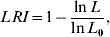
where ln L is the log-likelihood function for the model and ln L 0 is the log-likelihood computed with only a constant term, i.e. when all the slopes in the model are zero. The index provides an intuitive measurement for the goodness-of-fit similar to the R 2 in a classical regression. The index equals zero when all the slope coefficients are zero and is close to unity when the model correctly predicts the sample. The likelihood ratio indices for all seven specifications are reported in the final column of Table 2. For all specifications except specification IV, the likelihood ratio index is more than 0.27 and the hypothesis of all coefficients being zero is strictly rejected.
Specification IV excludes the LNSIZE variable in the regression, to examine the importance of collinearity with the remaining variables. It can be seen that the explanatory power of the regression drops substantially, and overall, the LNSIZE variable is regarded as an important variable that should not be excluded from the model. Specification VI includes a dummy variable for whether the institution was classified as a university pre-1992, which is the date on which a number of former polytechnics and colleges converted to full universities. This dummy variable takes the value of unity if the institution was a pre-1992 university and zero otherwise, and is related to both the age of the institution and also its size. It can be seen that the coefficient on the pre-1992 dummy is significantly negative, demonstrating that the pre-1992 universities have lower probabilities of financial distress. However, this variable is highly correlated with the size of the university, and, therefore the final model to be used to calibrate the insolvency risk is given in specification VII.
An alternative method to check for the predictive ability of the model is a 2×2 matrix of the hits and misses of a prediction rule such as

where  is the estimated probability from the model and F* is a threshold value or ‘cut-off’ point, which is usually set to be 0.5. In the context of a financial distress prediction model, a ‘hit’ means an observation is predicted to either be in financial distress or not, and the sample is also classified according to whether it is in actual financial distress or not. A ‘miss’ means a wrong prediction of the model for either a financially distressed or non-financially distressed firm. An error is Type-I if the estimated probability is greater than the cut-off point and the firm is non-financially distressed and Type-II if the probability is less than the cut-off point and the firm is financially distressed. This is an intuitive way to check the predictive power of the model since one can easily calculate the proportion of the sample that has been correctly predicted.
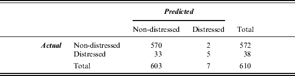
There is no criterion for the best cut-off point to use: it depends on the setting and on the criterion function upon which the prediction rule is based. In the multivariate discriminant analysis, a ‘good’ model is one that minimizes the sum of the two types of the errors. Table 3 shows the prediction results for specification VII in Table 2 using a 0.5 cut-off point.
Accuracy matrix for the logit model
The table depicts the performance of the logit model defined in equation (5) by looking at how many observations are correctly identified by the model as being financially distressed or non-distressed. The empirical specification used is Specification (VII) in Table 2. Predicted is the projected financial conditions identified by the logit model using a cut-off point of 0.5. Actual is the financial condition of an institution defined by the value of ABNML.
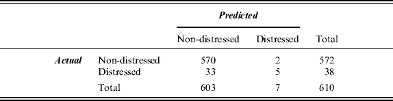
The table shows that the model predicts 575 out of 610, or 94.3%, of the observations correctly. Considered jointly with the likelihood ratio index of 0.27, the result is suggestive of a good fit. The finding that only five out of 33 institutions are correctly identified as in a financial distress is not surprising given the above arguments. Note that in this sample of 610 observations, only 38, or 6%, are identified as in financial difficulties (i.e. ABNML=1), which means that the average predicted probability of financial distress is also 0.06. As such, it may require an extreme configuration of regressors even to produce an estimated probability of 0.2, to say nothing of a value of 0.5. The reasoning is because a one half chance of financial distress for the HE sector is very high given that these are public sector institutions. Reducing the cut-off point will increase the correct prediction for distressed institutions but will also increase the predictive error for non-distressed institutions.Footnote 15
An alternative method of checking the performance of the model is to compare the results of our financial distress predictions with the results of other models within a similar sample. Recently the Education Guardian (10 July 2007) released a list based on information obtained from the Higher Education Funding Council for England under the Freedom of Information Act, naming 46 universities (about one-third of the total) from England on the HEFCE's list of colleges at risk of financial failure between 1998 and 2003. HEFCE had established a model to assess the financial performance of HE institutions, but this model was not publicly accessible. It contained four risk categories: first, institutions at immediate risk; second, at risk unless urgent action was taken; third, at risk unless action was taken; and, lastly, no risk.
The empirical financial distress prediction model in our paper is attempting to simulate the HEFCE prediction model using publicly available information. Our estimated probabilities are calculated from the logit regression and the 30% of institutions with the highest probabilities of financial distress are compared with the institutions identified by HEFCE as to fall within their first two risk categories, i.e. those institutions with immediate risk or at risk unless urgent action was taken.Footnote 16 For the set of the institutions that appear on both the HEFCE list and also in the dataset in this paper (that is, 36 out of 46 institutions), 25 institutions from the top 30 percentile from the sample appear at least once on the HEFCE list. This implies that the model used in this paper predicts over two-thirds of the universities that are likely to encounter financial distress correctly. Given that three year's worth of data from 1998 to 2000 that formed part of the Guardian list are missing from the HESA dataset in this research, the result provides strong evidence that the model used in this paper is appropriate and can be used to simulate the PPF insolvency risk and the risk-based levy in the next section.
5 The UK Pension Protection Fund
The UK Pension Protection Fund is a statutory fund run by the Board of the Pension Protection Fund, established under the provisions of the Pensions Act 2004. It was established to pay compensation to members of eligible defined benefit pension schemes, when there is a qualifying insolvency event in relation to the employer and where there are insufficient assets in the pension scheme to cover PPF levels of compensation. Existing schemes are charged an annual levy, which is a mixture of a scheme-based and a risk-based levy. The scheme-based levy is based on the scheme's pension liabilities and makes up 20% of the total pension protection levy. The risk-based levy is based on the scheme's underfunding risk and the insolvency risk of the sponsoring firm. The Pensions Act 2004 prescribes that after a transitional period, at least 80% of the pension protection levy (the levy) must be risk-based.Footnote 17 McCarthy and Neuberger (Reference McCarthy and Neuberger2005a) provide a model of a generic pension protection fund in which claims of the fund are infrequent but lumpy, and question whether the PPF will be able to build up sufficient reserves to be self-financing.
Together, the scheme-based levy and the risk-based levy make up the total PPF levy. From 2006/07 onwards, according to PPF (2006) the scheme-based levy is just proportional to the scheme's PPF protected liabilities L

where in 2006/07 the factor of proportionality is set as 0.00014. The long-term value of this parameter will be set to ensure that the scheme-based element comprises approximately 20% of the pension fund levy. Generally speaking, the PPF protected liability is the level of compensation that would be paid if the scheme were transferred to the PPF, it can either be the complete actuarial valuation according to section 179 of the Pensions Act 2004 or the adapted MFR (minimum funding requirement) liability (but only for 2006/07 is the MFR valuation eligible). Normally it should be smaller than the ‘true’ pension liabilities such as FRS17 or IAS19 liabilities.Footnote 18
In order to calculate the risk-based levy, the Board of the Pension Protection Fund considers the level of scheme underfunding (underfunding risk) and the likelihood of sponsoring employer insolvency (insolvency risk) and may also consider the asset allocation and any other risk factors that may be prescribed in regulations when setting the risk-based pension protection levy, which is reflected in the levy scaling factor the Board sets up and updates annually.
According to the PPF (2005b), the most recent risk-based levy (RBL) formula set by Pension Protection Board is calculated as

where U is the underfunding risk, P is the PPF assumed probability of insolvency, 0.8 is the percentage risk-based for levy year 2006/07, and c is the levy scaling factor, which will be set at 0.53 for levy year 2006/07. The Board decided to set the risk-based levy cap, after the application of the levy scaling factor, at 0.5% of section 179 liabilities in order to protect weaker schemes and a no risk-based levy is payable for schemes that are more than 125% funded on a PPF basis. McCarthy and Neuberger (Reference McCarthy and Neuberger2005b) criticize the proposed PPF levy structure in the Pension Protection Fund (2005a) on the basis that the risk-based structure relies on taxing the weakest schemes, which is infeasible as it will significantly increase the financial burdens for already distressed firms.
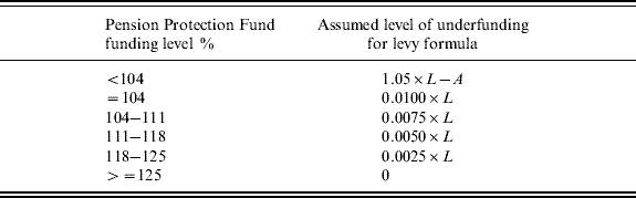
The underfunding risk is a measure of a participating scheme's pension fund deficit and this value is decreasing as the PPF funding level (scheme assets divided by liabilities) of the scheme increases. According to PPF (2005b), if a scheme is less than 104% funded on a PPF funding level, then the underfunding risk will remain the difference between 105% of the value of PPF liabilities and the value of scheme assets

For schemes that are funded above 104% on a PPF funding basis, the underfunding risk is tapered from 1% of PPF liabilities at the 104% funded level down to 0% in steps of 0.25%. This approach is detailed in Table 4.
Pension Protection Fund underfunding levy
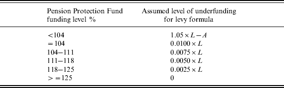
It can be seen that the greater the participating scheme's assets exceed its liabilities, the lower is the underfunding risk.
The PPF assumed probability of insolvency is calculated in conjunction with a third party provider. In 2006/07, this was Dunn & Bradstreet (D&B). The assumed probability of insolvency for the risk-based levy is calculated by identifying each participating scheme as being in one of the 100 risk bands related to the D&B failure score (the higher the score the lower the insolvency risk). Each risk band has an associated assumed probability of insolvency which is capped at 15%.
One of the complications regarding the risk-based levy arises from the structure of the eligible pension schemes. An eligible pension scheme covered by PPF can either be sponsored by a single employer (single-employer scheme) or more than one employer (multi-employer scheme) and according to the initial findings reported in the Pensions Protection Fund (2005a), many of the largest 500 pension schemes are multi-employer schemes with over 100,000 participating sponsoring employers between them. For a single-employer scheme, the Board only needs to consider the risks underlying this individual employer when calculating the pension protection levy. However, the risks faced by a multi-employer scheme may be different to those faced by single-employer schemes. The structure and the rules of different types of schemes have an impact on how the risk is shared among participating employers and, therefore, on the calculation of levy risk factors. Multi-employer schemes are classified into several categories according to the Pension Protection Fund (Multi-employer Schemes) (Modification) Regulations 2005 (or the Pension Protection Fund (Multi-employer Schemes) (Modification) Regulations (Northern Ireland) 2005) depending on whether the employers in the scheme are from the same or similar sectors (sectionalized/non-sectionalized) and whether the scheme has an option or requirement to segregate upon cessation of a participating employer.
For schemes with neither a requirement nor discretion to segregate on cessation of participation of an employer a LMS pension protection levy applies, under which the Board will not trigger an ‘assessment period’ until the last employer in that scheme becomes insolvent. For multi-employer sections/schemes with an option or requirement to segregate on cessation of participation, the scheme pays a ‘segmented’ levy, which means each sponsoring employer is only responsible for its own pension liabilities and, in the event of insolvency, only the insolvent firm's pension liabilities are transferred to the PPF, not the whole scheme.Footnote 19
For both LMS and segmented multi-employer schemes, the insolvency risk is calculated as the weighted average probability of insolvency for all participating sponsoring employers, but, in the case of an LMS arrangement, these probabilities are adjusted by a scaling factor δ<1 to reflect the degree of correlation across the employers in the scheme.Footnote 20
Hence, the scaling factor ensures that the LMS risk-based levy is lower, but raises a cross-subsidy issue, since an insolvent participating employer will be funded by the rest of the employers in the set of multi-employers. Consequently, there is a potential moral hazard problem, since managers of the participating pension schemes may behave irrationally or undertake risky activities once they realize that their pension fund is partially ‘insured’ by other firms in the scheme. Formally, for a segmented arrangement the levy is

For a LMS arrangement the levy is

The only difference between the risk-based levy for segmented and LMS schemes is the calculation of the insolvency probability P
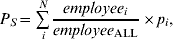
where p i is the assumed probability of insolvency for each participating employer/scheme. For all multi-employer LMS schemes, the assumed insolvency probability will be the same weighted average probability multiplied by a scaling factor defined as

with δ as the scaling factor.
6 Simulated PPF risk-based levies for USS under different arrangements
The Universities Superannuation Scheme Ltd publishes annual reports and accounts that provide information on the PPF levies in the statement of operating costs. For the year ended 31 March 2007, the total PPF levy for the USS, currently participating in the PPF according to a LMS basis, was £3.142 million, and this was the first year that the PPF split the levy into scheme-based and risk-based parts. According to the information provided by the USS, on 31 March 2006 it had a PPF liability of £22,214 million and its funding level on a PPF basis was 124%. Based on this information, one can use the risk-based levy formula given in equation (9) to calculate the implied aggregate probability of insolvency that the PPF applies to USS.
Using the information on the scheme's PPF liabilities and the PPF funding level provided by the USS, the scheme-based levy is 0.014% of the PPF liabilities, equal to £3.11 million, so the estimated risk-based levy for 2006/07 is £0.032 million.Footnote 21 As USS is 124% funded, the underfunding risk is 0.25% of PPF liabilities, equal to £55.52 million. Using the levy formula in equation (9), the implied P LMS is 0.14% for year 2006/07. Within the 100 insolvency risk bands imposed by the PPF, this is equivalent to a D&B failure score of 99, and is extremely low-risk in terms of the PPF's measure of insolvency risk.Footnote 22
However, consider an alternative measure of university insolvency risk implied by the Guardian list of 46 universities identified by HEFCE to be at risk of financial failure over the six-year period between 1998 and 2003. Now we obtain a completely different picture. Even if these 46 universities fell into financial distress no more than once over the five years, this would imply an average probability of financial failure of over 5%, a number that is over 30 times higher than the PPF implied probability of insolvency!Footnote 23 Of course one might argue that universities as public sector organizations will never be allowed to go bankrupt as the government will provide sufficient funds, in the event of insolvency, and the PPF implied probability is a reflection of this fact. However, this would imply inconsistencies in the use of the HEFCE term ‘at risk’, and/or the amounts of risk-based levies collected by the PPF from USS. Either some individual universities are at serious risk of financial failure and the PPF levy should reflect this, or universities are not at serious risk, in which case why does the PPF collect any risk-based levy from USS in the first place?
Other inconsistencies in the PPF funding have been emphasized by McCarthy and Neuberger (Reference McCarthy and Neuberger2005a, Reference McCarthy and Neuberger2005b) and Blake et al. (Reference Blake, Cotter and Dowd2007). McCarthy and Neuberger (Reference McCarthy and Neuberger2005a) show that there is a large chance the PPF will default on its liabilities if it sticks with its proposed levy structure and it will also raise severe moral hazard and agency problems. Blake et al. (Reference Blake, Cotter and Dowd2007) make similar arguments by comparing the PPF regulation with the regulatory system applied to other financial institutions like banks and insurance companies, as well as with the government-sponsored schemes in other countries such as the Pension Benefit and Guarantee Corporation in the US. McCarthy and Neuberger (Reference McCarthy and Neuberger2005b) criticize the risk-based levy for its reliance on weaker schemes to pay the levy, and propose an alternative levy structure through a less distortionary mechanism, which also considers seriously underfunded firms not being able to afford the PPF levy.
We will now proceed by assuming that there is a ‘real’ risk of some universities becoming insolvent, and we will simulate the appropriate aggregate P LMS that USS should pay, based on the individual insolvency probabilities of each institution calculated from our financial distress prediction model. The simulation uses the estimated probabilities from 2004/05 since this is the most recent HESA data available to us and we believe provides adequate approximations for the insolvency risk for the following years.
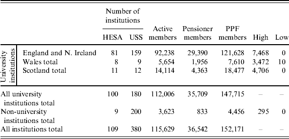
The information in USS 2005/06 Reports and Accounts on the participating members in each institution enable us to estimate the weighted average probability of insolvency across institutions. Table 5 shows the composition of USS member institutions and comparison with the available institutions reported in the HESA dataset. The membership numbers for a PPF scheme, according to the PPF (2005a), is the sum of active, deferred and pensioner members. As USS only provides splits of active and pensioner members of the scheme, the number of PPF members in our simulations used the sum of the active and pensioner numbers.Footnote 24 It can be seen that within the HESA data for 2005/06, 109 institutions can be matched with the USS membership statistics. Within these 109 institutions, only nine are non-university and the rest are all university institutions. Although losing 80 university institutions and most of the non-university institutions, the HESA data capture a total membership of 139,288, which includes more than 90% of the total PPF members.Footnote 25 We believe our sample is sufficiently representative to estimate the distribution of the PPF levies for USS.
Comparison of USS membership statistics
This table shows the composition of USS membership and the USS members that can be matched with the HESA HE Finance Plus dataset for year 2005/06. Under the column labelled Number of institutions, HESA is the number of institutions that are within the HESA Finance Plus dataset and are also USS participating institutions, and USS is the total number of USS participating institutions. The number of PPF members is the sum of active and pensioner members; High and Low are institutions with the highest and lowest number of PPF members.
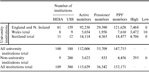
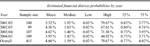
Table 6 shows the basic distribution of the estimated financial distress probabilities from equation (5). The mean probability of financial distress for the entire four-year sample is 4.6%, which matches the probability implied by the Guardian list of 46 universities identified as being at risk (implying approximately 5% probability of annual insolvency risk). In Table 6, the mean estimated probability of financial distress is decreasing for the four sample years, and is supportive of the claim made by the HEFCE in the Education Guardian (2007) that HE institutions have improved their finances over the period.
Statistics for estimated probabilities of financial distress
This table reports the yearly simulated probabilities of insolvency for UK HE institutions (that participate in the USS) estimated by the logit model defined in equation (5) using the coefficient estimates in specification (VII) of Table 2 from financial years 2001 to 2004. Low and High stand for the lowest and the highest value, and 25% and 75% stand for the 25 and 75 percentile of the estimated values, respectively.
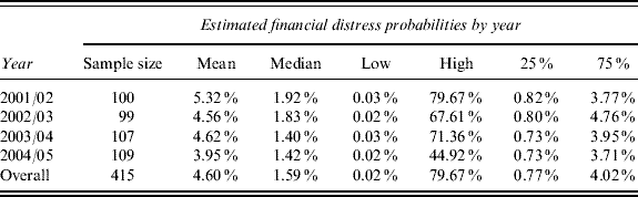
Using the logit model in equation (5), we estimate the individual insolvency risk associated with each of the universities participating in USS. We then compute the aggregate insolvency risk as the weighted average of these probabilities using equation (13). We calculate this aggregate probability P S, to be 1.20%, and since the current USS participation in the Pension Protection Fund is on a LMS basis, with a scaling factor δ=0.9, then from equation (14), the simulated P LMS is 1.1%. This is greater than the implied insolvency probability P LMS of 0.14% obtained from the aggregate USS accounts.
By comparing these two sets of probabilities, our estimates suggest that currently USS member institutions appear to be paying less than the fair risk-based levy. However, this is because during the initial phase of the PPF the risk-based levies are much lower as a proportion of the total levy than the intended steady-state value. The implication is that if USS paid the same total levy but where the risk-based component was four-fifths of the total, then USS would be paying substantially more than its fair risk-based levy.
Having assessed whether the risk-based levy paid by USS members is fairly priced, we now turn to the implicit cross-subsidy under a LMS PPF levy relative to a segmented arrangement. As we have seen, as a multi-employer defined benefit pension scheme, USS contributes to the PPF on a LMS basis and benefits from the less-than-perfect positive correlation between the solvency of the schemes' institutions. However, the scaling factor of 0.9 for associated schemes means that the total risk-based levies do not differ dramatically whether the USS participates as an LMS scheme or as a segmented scheme, since the scaling factor is so close to unity. The main difference between the LMS and segmented participating methods arises from the cross-subsidy among the schemes – under LMS, institutions with lower risks pay a higher pension protection levy for those more financially distressed institutions. In addition, whenever these riskier institutions become insolvent, the remainder of the institutions will be obliged to fund those insolvent schemes. Evidence of the existence of the cross-subsidy phenomena would be a highly asymmetric distribution of risk-based levies paid by individual participating institutions, skewing towards lower values (i.e. left-hand towards the mean value). This idea is the starting point for the empirical design to compare the two alternative risk-based levies.
In order to simulate the distribution of risk-based levies for individual institutions, we first need to estimate imputed values for PPF liabilities for each institution. These are imputed values since USS is constituted as a mutual organization and there is no provision within USS rules for a segmentation arrangement. USS Ltd publishes in its annual report and accounts membership statistics for all participating institutions each year, which include the number of the members in each institution as well as the value of the USS pension assets and liabilities under FRS17 Retirement Benefit. We estimate pension liabilities for individual member institutions on the basis of the number of USS members within that institution, calculated as

where subscript i indicates the ith institution and subscript USS stands for the data for the entire Universities Superannuation Scheme. Assuming the same funding level with the USS (124%) for all participating institutions, the underfunding risk is, therefore, 0.25% of the PPF liabilities for each institution according to Table 4. Moreover, considering that the USS members within the HESA dataset are only proportional to the total number of USS members as shown in Table 5, we scale the total USS pension liabilities by the ratio of the total number of HESA-USS members to the total number of USS members.Footnote 26
From Table 6 we know that the average estimated probability of insolvency for 2004/05 is 3.95%, which is lower than the average for 2005/06 using samples that can be retrieved from the USS annual report only (5.9%, results not reported). This is because some institutions with extremely high estimated probabilities cannot be retrieved from the USS membership data, which are then excluded from the simulation. Recall that the weighted average simulated probability of insolvency was 1.2% – much lower than the arithmetic mean. This finding confirms the result from the logit regression that it is the small institutions that are more likely to encounter financial difficulty, and these institutions will have a low weight in the average probability.
If the weighted average simulated probability were scaled properly as a LMS associated scheme by 0.9, this would imply that the USS insolvency probability is 1.08%. Using these weighed average probabilities in the 100 risk bands to calculate the PPF assumed probability of insolvency, the USS falls between the 74th (with assumed insolvency probability of 1.11%) and 75th band (assumed probability of 1.06%), which is consistent with the view that universities have a low risk of financial failure. The fairly priced risk-based levy simulated from PPF formula equation (9) should be £255,542 for 2006/07, which works out to an average of £1.70 for each individual USS member.
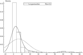
Figure 1 depicts the histogram and the density for the distribution of the estimated levies per USS member using forecasted probabilities of financial distress for 2004/05. The numbers for each institution are listed in Appendix 1. Using levy per member rather than levy per participating institution guarantees that the value of the levy does not pick up the size of the institution and the levy reflects directly the probability of financial distress for each institution. Compared to the normal distribution, represented by the dashed line, the distribution of the simulated risk-based levy is obviously asymmetric and positively skewed (i.e. to the left). From the histogram describing the frequencies for different levy values, the bin-range with the highest frequency also has the smallest value, which is between £0 and £4 per member and most of the distribution is clustered within the levy below £10 per member. The peak for the probability density function for the risk-based levy, is just over £2, is significantly lower than that of the sample mean of £6, which is depicted by the highest point of the normal distribution. This can be seen more intuitively from Figure 2, where the distribution of the simulated risk-based levy is compared to that of the normal distribution.
Histogram and density for the simulated risk-based levy (per member) against normal distribution

Distribution of the simulated risk-based levy against normal distribution

These findings suggest that under a segmented participating rule for the PPF, most of the USS member institutions would pay a relatively low risk-based levy. However, the fact that the levies with the highest frequencies are less in value than the mean levy across all USS members means that schemes paying higher levies are contributing more than those paying lower levies. Schemes that pay high levies are normally larger institutions with high pension liabilities and therefore larger underfunding risk and from the regression results they are usually low-risk institutions.
The levy paid by the USS under the LMS rule is just a weighted average of individual levies and, therefore, this is evidence of the cross-subsidy amongst the participating schemes where low-risk institutions provide a free insurance to those with higher risk of failure because they have to use their own assets to pay for the deficits of the high-risk institutions as long as the USS as a whole stays solvent. This cross-subsidy is a cost to the financially secure universities. The LMS arrangement is a consequence of the mutual organization of USS, but the cross-subsidy disadvantages, may be outweighed by other advantages of mutuality.
We note that there are other advantages from USS being organized as a mutual institution. First, there may be economies of scale in pension fund management, from having a single large pension fund, rather than a large number of smaller ones. However, the optimal arrangements for pension fund management are unclear, since the economies of scale advantages need to be weighed against any second-best principal-agent considerations in a delegated portfolio management environment (Sharpe, Reference Sharpe1980; Lakonishok et al., Reference Lakonishok, Shleifer and Vishny1992; Kapur and Timmermann, Reference Kapur and Timmermann2005; Tonks, Reference Tonks, Clark, Munnell and Orszag2006; van Binsbergen et al., Reference Binsbergen, Brandt and Koijen2008). Second, the existence of an industry-wide pension scheme allows for flexibility in job turnover across the participating institutions (Dorsey, Reference Dorsey1995; Blake and Orszag, Reference Blake and Orszag1998; Blake, Reference Blake2000). Thirdly, it is well known from the corporate governance literature (Smith and Stulz, Reference Smith and Stulz1985; Guay, Reference Guay1999; Sudarasanam and Huang, Reference Sudarsanam and Huang2006), that risk-averse executives, whose human capital is tied up in their organization, under-invest in risky projects: a segmented university pension scheme might result in decision-makers at universities making sub-optimal investment decisions.
7 Robustness checks
An alternative measure of financial distress in HE institutions are variables related to the earning power of that institution. EBIT (earnings before interest and taxes) are a natural candidate since they are linked to both stock-based and flow-based aspects of the financial distress definition: a negative EBIT reflects the firm's inability to generate positive cashflows to cover future contractual and operating expenses and will eventually reduce the firm's assets. They are an indicator of poor performance and as they determine the fair value of firms' assets, are negatively related to firms' solvency. The model also adopts the logit model in Ohlson (Reference Ohlson1980) and Lennox (Reference Lennox1999) and uses two-year consecutive negative earnings as predictors, which is equivalent to the independent variable NEGTWO t in equation (3).
As the model uses EBIT as the proxy for financial distress, it captures the components of earnings, normally equal to the difference between incomes and expenditures. We have already discussed that income of HE institutions mainly consists of funding council grants, tuition fees, and research grants and contracts. Expenditure can be decomposed into staff costs, other operating expenses, and interest payable. The remaining variables are typical control variables in bankruptcy prediction models, including LNSIZE, WCTA, and TLTA as defined in Section 2. The final model is in the form of

where
INCOME 1=funding council grants/total asset
INCOME 2=tuition gees & education grants/total asset
INCOME 3=research grants & contracts/total asset
INCOME 4=other income/total asset
COST 1=staff cost/total asset
COST 2=other operating expenses/total asset
COST 3=interest payable/total asset
and the subscripts t and t−1 imply that the data from the previous year are used to predict the EBIT value in the current financial year. Variables related to income should be negatively correlated to the probability of continuous low earnings and the opposite should hold for variables depicting the costs. The rest of the explanatory variables should have the same sign as in the original model.
Table 7 reports the estimates of the parameters from the logit regression in equation (16) and the predicted probability of financial distress. As expected variables related to the income and expenditure streams are significantly correlated with the earnings pattern at 99% confidence interval, higher income will lower the probability of continuously poor financial performance and vice versa for the cost-related variables. The combined coefficients on incomes and expenditures effectively cancel out. In all four specifications, the size of an institution appears to be unimportant in predicting the probability of consecutive negative earnings. This might be because other variables scaled by total assets may capture the statistical significance of the size variable. However, size is still insignificant when regressed as the only explanatory variable (results not reported). Working capital is significant and is negatively correlated with the probability of consecutive negative earnings, as expected. This implies that working capital is important in explaining the income pattern of HE institutions. The total liabilities/total assets ratio is insignificant and with the wrong sign, indicating that the dependent variable is a poor proxy for financial distress in the HE sector. The estimated financial distress probabilities are more than 17% for all four specifications, and are much higher than the 6% mean probability predicted in the original model using unanticipated funding council grants as the predictor of financial distress.
Robustness tests using continuous negative earnings as the financial distress predictor
The table represents the results for the logit regression described in equation (16) with dependent variable as Pr (NEGTWO t=1|X), where X is the set of explanatory variables. LNSIZE is the log of total book assets (TA). WCTA is the ratio of working capital to total assets. CLCA is current liabilities divided by current assets (CA). CLTA is current liabilities divided by total assets. LLTA is long-term liabilities divided by total assets. TLTA is the ratio of total liabilities (CL+LL) to total asset. INCOME and COST are as defined in equation (16). Specification (I) is the basic model as in Ohlson (Reference Ohlson1980). Specification (II) adds working capital in the regression and specification (III) includes current liabilities from specification (II). Specification (IV) only includes long-term liabilities as compared to specification (I). Robust t-statistics are reported in parenthesis and *, **, *** stand for 10%, 5%, and 1% significance levels, respectively.

In summary, using consecutive negative earnings as a predictor of financial distress partially confirms the relation between financial statement variables and the probability of financial distress. However, it performs less well than the model using abnormal funding council grants as the proxy for financial distress both in the explanatory power of important variables and the predicted probability of financial distress.
8 Conclusions
This paper has estimated the risks of financial distress of UK universities, and has then used these estimates to examine the basis of the annual levies paid to the UK's Pension Protection Fund by the Universities Superannuation Scheme, a multi-employer scheme covering 391 universities and related institutions. We have investigated the trade-off between the two PPF participating arrangements for multi-employer pension schemes, namely last-man-standing and segmented levies, using a sample dataset from participating USS HE institutions We estimated an insolvency prediction model, using the allocation of unanticipated funding council grants as the proxy for financial distress, and we found that financially distressed institutions are smaller in size, with higher leverage ratios and lower earnings, which is consistent with the conventional results from the bankruptcy prediction literature. As a check on the predictive accuracy of our model, we compared the institutions identified as being in financial distress with the list of HE institutions at risk of financial failure disclosed by Education Guardian (10 July 2007). We find that over two-thirds of the universities from the Guardian list can be retrieved by our financial distress prediction model.
We then used the information provided by USS Annual Reports to calculate the implied probabilities of financial distress. Then we compared this implied probability with the simulated financial distress probability using our empirical specifications to assess whether the PPF levies are fairly priced. Our estimates suggest that in 2006/07 USS member institutions appeared to be paying less than the fair risk-based levy. However, this is because during the initial phase of the PPF, the risk-based levies were much lower as a proportion of the total levy than the intended steady-state values. The implication is that if USS had paid the same total levy but where the risk-based component was four-fifths of the total, then USS would have been paying substantially more than its fair risk-based levy.
In addition, by examining the distribution of risk-based levies for individual institutions under a simulated segmented PPF arrangement, we find a highly asymmetric distribution skewed towards lower values. This provides evidence of significant cross-subsidies under the current LMS levy between participating USS institutions from those institutions with better financial conditions to financially distressed institutions. Of course, there may be advantages in USS mutuality, in terms of: economies of scale in pension fund management, flexibility in job turnover, and appropriate alignment of goals of the institutions and their executives. However, the implied segmented levies make explicit the cross-subsidy between the financially stronger and weaker HE institutions.
Appendix 1

The total sample of the Guardian list contains 180 (English) universities of which 43 are deemed ‘at risk’. From our table of 109 institutions (including non-English universities), 20 institutions can be found in the Guardian list. The entry ‘yes×n’ means either the institution has been identified in the list n times or the institutions have now merged as one. Many of the missing institutions have subsequently merged with larger universities that are not now at risk (e.g. Bretton Hall which is now part of University of Leeds) or they no longer exist. The rest of the missing institutions are due to not being identified from the USS membership data.
 is equal to its mean. A naive t-statistic would be
 and a t value greater than 2 means we can reject the hypothesis at briefly 95% confidence level.