2. TEST PROCEDURES

Consider the univariate time series process {y_t}, generated according to

where φ(z) ≡ (1 − φ₁ z)(1 − φ₂ z) is a second-order polynomial in the lag operator L; L^ky_t ≡ y_t−k, k = 0,1,2,…. We follow Haldrup (1994, p. 110) and assume that the innovations {ε_t} are weakly dependent and heterogeneous, satisfying the well-known strong mixing conditions of, inter alia, Phillips (1987, Assumption 2.1, p. 280) with long-run variance σ².

As demonstrated in Hasza and Fuller (1979), (2.1) may be equivalently reparameterized as

where (γ₀^*, γ₁^*) and (γ₀, γ₁) form a one-to-one mapping, ρ₁ = −(1 − φ₁) × (1 − φ₂), and ρ₂ = (φ₁φ₂ − 1). Our interest centers on testing the null hypothesis that y_t ∼ I(2), namely,

such that the process requires double differencing to attain stationarity, against the alternative that y_t is either explosive, I(1) or I(0),

Consequently, a test for H₀ of (2.3) against H₁ of (2.4) can be based on a joint F-type test for the exclusion of both the regressors y_t−1 and Δy_t−1 from (2.2).

We explore the impact of the (observable) starting values of the process, y₀ and y₋₁, on the null distributions of test statistics for double unit roots, via three important cases.

Case 1. y₀ = μ₀ and y₋₁ = μ₋₁, with μ₀ and μ₋₁ fixed constants.

Case 2. y₀ and y₋₁ are both O_p(1) random variables.

Case 3. For some κ > 0,

.

Case 1 is assumed by Hasza and Fuller (1979) and Sen and Dickey (1987), the latter imposing further that μ₀ = μ₋₁. To illustrate Case 2, two particular examples seem useful: first, the case where y₀ = ε₀ and y₋₁ = ε₋₁, that is, where the initial values have variances equal to that of the shocks; second, where, under H₀ of (2.3), the history of the process stretches back to some point in the finite past, namely,

, where m is a strictly positive finite constant. For finite T, it is always possible to find values of m and κ such that Cases 2 and 3 coincide. However, this is not the case asymptotically because under Case 3 y₀ and y₋₁ are both of O_p(T^3/2); that is, the starting values are of the same stochastic order as the data points y₁,…, y_T. The asymptotic distribution theory under Case 3 is therefore likely to give a better approximation to the finite-sample null behavior of the statistics of Section 2 under random starting values than is that under Case 2. In the standard unit root literature the analogue of Case 3 has also been widely adopted for related reasons (see, inter alia, Phillips and Lee, 1996; Canjels and Watson, 1997). Although other assumptions could be made concerning the mechanism generating y₀ and y₋₁ we believe that Case 3 is of most practical relevance because here the starting values are generated by the same underlying process as {y₁,…, y_T}. However, our main focus here is to identify those double unit root tests that are exact similar to the initial conditions. If we then restrict ourselves to such tests, what we assume about the initial conditions (provided they are well defined) becomes irrelevant.

2.1. The Hasza and Fuller Test

Hasza and Fuller (1979) develop a test for H₀ of (2.3) based on indirect detrending by using the standard OLS regression F-statistic for the exclusion of both y_t−1 and Δy_t−1 from (2.2), which we denote by F₄^OLS. Hasza and Fuller (1979) also consider the case where the linear trend term is omitted from (2.2). In what follows we will refer to this restricted test regression as (2.2a) and to the corresponding F-statistic as F₂^OLS.¹

Notice that, by the familiar Frisch–Waugh theorem, F₄^OLS is numerically identical to the F-statistic obtained from a regression of Δ²y_t on the variables

of (3.6) and (3.7), respectively, whereas F₂^OLS is numerically identical to the statistic from a regression of Δ²y_t on the variables y_t−1 and

of (3.2) and (3.5), respectively.

Alternatively one can use direct demeaning via the regression model,²

As shown in Section 3, Δ²y_t ≡ Δ²y_t and Δy_t−1 ≡ Δy_t−1. Moreover, notice that

.

where

, is y_t demeaned, and compute the OLS F-type test for the exclusion of y_t−1 and Δy_t−1 from (2.5). This test will be denoted F₁^OLS in what follows. In the case where the linear trend is retained in (2.2), a similar alternative is to calculate the F-statistic from the OLS regression of

, where

is y_t demeaned and detrended; we will refer to this regression as (2.5a) and to the associated F-test as F₃^OLS. However, contrary to what is observed for standard unit root tests, neither F₁^OLS and F₂^OLS nor F₃^OLS and F₄^OLS are equivalent, even asymptotically, as will be shown subsequently.

2.2. The Simple Symmetric Test

Considering first the no-trend case, it follows from Fuller (1996) and Sen and Dickey (1987) that the SSLS estimator

from (2.2a) is given by

, where ω = diag(½,…,½) is a 2T × 2T diagonal weight matrix, X comprises the second (with the term −μ omitted) and third columns from Table 2 of Sen and Dickey (1987, p. 465) augmented by a column of ones, and Y ≡ (Δ²y₁,…, Δ²y_T, Δ²y_T,…, Δ²y₁)′. From this we obtain that the SSLS estimators for ρ₁ and ρ₂ in the case of indirect demeaning are given by,

³

Notice that Sen and Dickey (1987) set ω = I_2T. However, the test statistics they propose will clearly yield identical critical regions, but do not possess identical distributions, to those in (2.6) and (2.7); see Remark 4.7.

Defining R = [0_2×1 : I₂] , the F-type test for the joint significance of ρ₁ and ρ₂ is given by

where

is the associated SSLS estimator of σ² (see Fuller, 1996, p. 415). Similarly, the SSLS t-statistics

for testing ρ_j = 0, j = 1,2, may be defined as

where R₁ = (0 1 0) and R₂ = (0 0 1).

For the case where direct demeaning is employed, the SSLS estimator from (2.5) is given by

, where

comprises the second and third columns from Table 2 of Sen and Dickey (1987, p. 465) with the term μ replaced by the sample mean y. As discussed in Fuller (1996, p. 416), and in contrast to the Hasza and Fuller (1979) procedure,

is asymptotically equivalent to

obtained using indirect demeaning previously. Consequently, the F-statistic

and corresponding

, are also asymptotically equivalent to those given for the case of indirect demeaning previously.

The corresponding tests that allow for a linear trend may be straightforwardly obtained from SSLS estimation of (2.2) and (2.5a). We denote these statistics by F₄^SSLS and F₃^SSLS, respectively. However, here the two approaches are not equivalent, even asymptotically. In both cases

coincides and has an expression similar to (2.6) except that the demeaned y_t−1, y_t−1, is replaced by demeaned and detrended y_t−1,

. For

, the expression in (2.6) is obtained for the SSLS estimation of (2.2), but where the tests are obtained from SSLS estimation of (2.5a) the expression for this statistic is given by (2.6) but with

replacing Δy_t. For details see the Appendix of Rodrigues and Taylor (2002).

3. DIRECT AND INDIRECT DEMEANING AND DETRENDING

Under H₀ of (2.3) it is straightforward to show that

Defining t ≡ (T + 1)/2, it follows that the demeaned process y_t ≡ y_t − y may be written as

where

As a consequence of (3.2),

Moreover, Δ²y_t = Δ²y_t = ε_t.

It is seen from (3.2) that the demeaned process {y_t} depends on the difference between the initial conditions, (y₀ − y₋₁), with this dependence growing linearly with t. The first difference of the demeaned process {Δy_t} also depends on (y₀ − y₋₁), but here the dependence is constant over the sample. In contrast to (3.4), if we demean Δy_t itself (as will be the case with the use of indirect demeaning) it is straightforward to establish that

which is invariant to the starting values.

It is clear from (3.2) and (3.4) that the F₁^OLS and F_j^SSLS, j = 1,2, tests of Section 2 will not be exact similar under either Cases 2 or 3 but only under Case 1 where μ₀ = μ₋₁ (cf. Sen and Dickey, 1987). As regards the F₂^OLS test, although this too is not exact similar, we might expect it to be less affected than the F₁^OLS statistic by virtue of the invariance of

to the initial values; cf. (3.5). This conjecture appears to be supported by the numerical results reported in Section 5, where F₂^OLS is shown to be considerably less sensitive to the starting values. In the next section we show that tests based on the F_j^OLS and F_j^SSLS, j = 1,2, statistics are asymptotically similar under Cases 1 and 2 but not under Case 3. In Case 3, the limiting null distributions of the statistics are shown to depend on the history parameter κ.

Although the demeaned data y_t depend on the initial values of the process, it is straightforward to show that the demeaned and detrended data,

, satisfy

where

is as defined in (3.3) and, hence, is invariant to the initial conditions, as will be

. Moreover, it is also easily demonstrated that the demeaned and detrended Δy_t satisfies

which is also invariant to these parameters. Consequently, the F₃^OLS, F₄^OLS, and F₃^SSLS statistics of Section 2 will all yield exact similar inference. In contrast, the F₄^SSLS test is not exact similar with respect to y₀ and y₋₁, as is clear from the discussion at the end of Section 2.2. Hence, one should not use indirect detrending in the context of the SSLS tests.

Remark 3.1. Notice from (3.1) that by considering the transformation

we obtain transformed data {y_t^*} that are exact invariant to the initial conditions under H₀ of (2.3). Consequently, the F-statistics calculated from the OLS and SSLS regressions of Δ²y_t^* on y_t−1^* and Δy_t−1^* will yield exact similar tests with respect to y₀ and y₋₁. We will refer to these statistics as F_*^OLS and F_*^SSLS, respectively. It is easily demonstrated that the limiting null distribution of F_*^OLS is as given for the

statistic in Theorem 1 of Haldrup (1994, pp. 111–112), whereas that of F_*^SSLS is as given for the

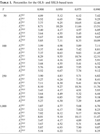
statistic in Theorem 1 of Shin and Kim (1999, p. 68). Semiparametric modifications to these statistics may be carried out in the manner outlined in Haldrup (1994, pp. 112–113) and Shin and Kim (1999). Appropriate critical values for tests based on the modified F_*^OLS and F_*^SSLS statistics are therefore as given for the statistic labeled Φ₁(2) in Table 4.1 of Hasza and Fuller (1979, p. 1116) and in Table 1, which follows, respectively.

Percentiles for the OLS- and SSLS-based tests

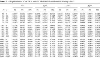
Size performance of the OLS- and SSLS-based tests under random starting values

4. ASYMPTOTIC REPRESENTATIONS

Suppose that y_t is generated according to (2.1) under H₀ of (2.3) with y₀ and y₋₁ generated according to Case 3. We then have that

as T → ∞, where V(.) is a standard Brownian motion; ⇒ is used throughout this paper to denote weak convergence of the associated probability measures. Using Donsker's theorem (see Billingsley, 1968), it follows using (4.1) that

Remark 4.1. Notice that under both Case 1 and Case 2, T^−3/2y_j, j = 0,−1 and T^−1/2(y₀ − y₋₁) are of o_p(1).

Now, from (3.1) we have that

Consequently, from (4.1), (4.2), Equation (2.3) of Haldrup (1994, p. 111), and applications of the continuous mapping theorem we obtain that as T → ∞,

where [·] denotes the integer part of its argument, W(·) is a standard Brownian motion independent of V(·), and

are (independent) integrated Brownian motions. The result in (4.3) is the building block of the results that are stated subsequently. It also serves to illustrate the difference between Cases 1 and 2 and Case 3 on the asymptotic distribution theory, because under Cases 1 and 2 the first two terms of the right member of (4.3) vanish; cf. Remark 4.1.

In Lemma 4.1, we now detail the limiting behavior of the sample regression quantities used in constructing the OLS and SSLS statistics of Sections 2.1 and 2.2. The proof of Lemma 4.1 is available from the accompanying working paper, Rodrigues and Taylor (2002). We explicitly state the limiting results only for Case 3 of the initial values. However, Cases 1 and 2 obtain directly from the results that follow simply by setting κ = 0 throughout, noting that V(0) ≡ 0.

LEMMA 4.1. Let {y_t} be generated by (2.1) under H₀ of (2.3), with y₀ and y₋₁ generated according to Case 3. Then as T → ∞,

where W(·), V(·), W^*(·), and σ² are as defined previously,

where

, and κ is nonnegative.

Remark 4.2. Notice from Lemma 4.1 that the directly and indirectly demeaned and detrended regression quantities used in constructing the double differencing test statistics of Section 2 have different large-sample properties under H₀ of (2.3). This contrasts sharply with the standard unit root ADF statistics where the direct and indirect methods of demeaning/detrending are asymptotically equivalent. As an example, from parts (iii) and (iv) of the lemma we see that the scaled partial sum of the directly demeaned quantity Δy_t weakly converges to the sum of two independent Brownian motions (one of which appears only where κ > 0), whereas the corresponding scaled partial sum of the indirectly demeaned quantity

weakly converges to a demeaned Brownian motion.

We now provide limiting null representations for the Hasza and Fuller–type statistics and simple symmetric statistics of Section 2. These results follow from Lemma 4.1 after lengthy but tedious algebra; proofs are provided in Rodrigues and Taylor (2002). Again, although results are explicitly stated only for Case 3 of the initial values, results for Cases 1 and 2 obtain by setting κ = 0 throughout.

4.1. The Hasza and Fuller Statistics

In Theorem 4.1 we provide representations for the limiting null distribution of the Hasza and Fuller (1979) F₁^OLS and F₂^OLS statistics of Section 2. Corresponding representations for the F₃^OLS and F₄^OLS statistics are subsequently discussed in Theorem 4.2.

THEOREM 4.1. Under the conditions of Lemma 4.1 the F₁^OLS and F₂^OLS statistics of Section 2.1 have the following limiting distributions:

Remark 4.3. If the initial values are generated according to either Case 1 or Case 2 of Section 2, such that κ = 0, and σ² = σ_ε², as happens when ε_t ∼ IID(0, σ²), then the right member of (4.4) corresponding to F₂^OLS reduces to the equivalent

representation, formulated in terms of linear combinations of independent and identically distributed (i.i.d.) N(0,1) variates, given in Corollary 3.1 of Hasza and Fuller (1979, p. 1115). Hasza and Fuller derive this result under Case 1 with i.i.d. errors. Theorem 4.1 therefore demonstrates that their result holds under much weaker conditions on the initial values. However, although they derive their results under Case 1, Hasza and Fuller subsequently suggest (p. 1119) that these representations hold irrespective of the initial values. Theorem 4.1 demonstrates that this is not the case and that here the limiting representations of the Hasza and Fuller statistics depend on the history parameter κ.

Remark 4.4. The representations for the limiting null distributions of F₁^OLS and F₂^OLS given in Theorem 4.1 do not coincide, even for κ = 0. The former is a functional of a demeaned integrated Brownian motion and a standard Brownian motion, whereas the latter is a functional of a demeaned integrated Brownian motion and a demeaned Brownian motion that, for κ = 0, coincides with the representation given in Haldrup (1994, p. 113). This disparity is confirmed by a comparison of the percentiles given in Table 1. This disproves the claim made in Haldrup (1998, p. 611) that the two detrending procedures “are going to deliver the same results.”

THEOREM 4.2. Under the conditions of Lemma 4.1 the F₃^OLS and F₄^OLS statistics of Section 2.1 have the following limiting distributions:

Remark 4.5. As with the F₁^OLS and F₂^OLS statistics, the limiting null distributions of the F₃^OLS and F₄^OLS statistics are not equivalent, again contrary to what is claimed in Haldrup (1998, p. 611). The representation given for F₄^OLS coincides with that given in Haldrup (1994, p. 113). However, the limiting null distributions of F₃^OLS and F₄^OLS, unlike those of F₁^OLS and F₂^OLS, do not involve V(κ). Recall that these statistics are exact invariant to the initial values; cf. Section 3.

Remark 4.6. In light of Remarks 4.4 and 4.5, the testing strategy proposed by Haldrup (1994, p. 115) requires modification: either Haldrup's step 2 is altered to allow use of a test regression with the necessary deterministic variables included rather than “prior detrending of the series” (1994), or alternatively step 5 needs to accommodate the use of the critical values for the F₁^OLS and F₃^OLS statistics presented in Table 1. See also the discussion on semiparametric modifications of the OLS-based statistics in Section 6.

4.2. The Simple Symmetric Statistics

In Theorem 4.3 we now provide representations for the limiting null distribution of the SSLS statistics of Section 2.2 appropriate to the no-trend case. The following results are appropriate to the SSLS estimation of both (2.2a) and (2.5), that is, to the cases where demeaned data are used and where a column of ones is included in X, respectively. A formal proof of this result is provided in Remark A.3 of the Appendix to Rodrigues and Taylor (2002). Limiting null representations appropriate to the trend case are subsequently detailed in Theorem 4.4.

THEOREM 4.3. Under the conditions of Lemma 4.1, the SSLS t-statistics,

, have the following large-sample distributions:

Remark 4.7. Notice that the right members of (4.6) and (4.7) both depend on the history parameter κ. If, however, κ = 0, as happens when the initial values are generated according to either Case 1 or Case 2 of Section 3, then η₂(0) coincides for the case where ε_t ∼ IID(0, σ²) with the limiting distributions given in Fuller (1996, Theorem 10.1.7, p. 570) for the simple symmetric studentized statistic obtained from a first-order autoregression (with no constant) under the unit root (I(1)) null. Moreover, in such cases,

is also equivalent to the corresponding distribution provided by Sen and Dickey (1987, p. 466).

From (2.7) it can be established that the scaled second moment matrix from the SSLS estimation of (2.2a) and (2.5) is asymptotically block diagonal between y_t−1 and Δy_t−1 (see Rodrigues and Taylor, 2002, equation (A.29)). Consequently, unlike the Hasza and Fuller (1979) F₁^OLS and F₂^OLS statistics, the limiting null distributions of the F₁^SSLS and F₂^SSLS statistics of Section 2 are identical and are simply the average of the square of the limit distributions in (4.6) and (4.7).

COROLLARY 4.1. Under the conditions of Lemma 4.1,

We now turn to the statistics derived from the SSLS estimation of (2.5a) and (2.2). We demonstrate in Theorem 4.4 that although the limiting null distributions of the test statistics on ρ₁ are equivalent across these two cases, the statistics on ρ₂, and hence the joint statistics, F₃^SSLS and F₄^SSLS, are not. Again, the scaled second moment matrix in both of these cases is block diagonal between the stochastic regressors.

THEORM 4.4. Under the conditions of Lemma 4.1, the

statistics obtained from SSLS estimation of (2.5a) have the following large-sample distributions:

and the corresponding statistics obtained from SSLS estimation of (2.2) satisfy

where

Remark 4.8. In accordance with their exact similar properties demonstrated in Section 3, the limiting representations in (4.9)–(4.11) of Theorem 4.4 do not depend on V(κ), regardless of what is assumed about the starting values y₀ and y₋₁. This also holds true for

in (4.12), obtained from the SSLS estimation of (2.2). However, the limiting null distribution of the

statistic from SSLS estimation of (2.2), η₃, is identical to that of the corresponding statistic from the SSLS estimation of (2.5); that is, it, and consequently the joint statistic F₄^SSLS, is not asymptotically pivotal, except where κ = 0.

6. SEMIPARAMETRIC TESTS

It is clear from Theorems 4.1–4.4 that the limiting null distributions of the OLS and SSLS statistics depend on the nuisance parameters σ² and σ_ε². Following Haldrup (1994) and Shin and Kim (1999) we can modify these statistics to obtain statistics with limiting null distributions that correspond to those in Theorems 4.1–4.4 appropriate to those where ε_t ∼ IID(0, σ²) and, hence, σ² = σ_ε². Consequently, the critical values provided in Table 1 can then be used for the modified statistics (where the tests are similar with respect to the starting values) with these remaining asymptotically valid under a wide class of weakly dependent and heterogeneously distributed errors, {ε_t}.

Consider first the Hasza and Fuller–type statistic based on directly demeaned data, F₁^OLS. Following Haldrup (1994, p. 112) we define the following directly demeaned quantities:

Following Haldrup (1994, pp. 112–113) consider now the transformed statistic

where

is the long-run variance estimator of Haldrup (1994, equation (3.2), p. 112) with

the OLS residuals from estimating (2.5),

. Then, under the conditions on {ε_t} given in Phillips (1987) and Phillips and Perron (1998) to ensure that the estimators

are consistent under the null, it follows exactly as in Haldrup (1994, Theorem 2, p. 112) that Z(F₁^OLS) will have the limiting null distribution given by that of F₁^OLS in Theorem 4.1 with σ² = σ_ε². The transformed F₁^SSLS statistic of Shin and Kim (1999),

where

, will similarly obtain the null distribution for F₁^SSLS in Corollary 4.1 with σ² = σ_ε². Notice that these representations will still involve the limiting process V(κ) arising from the initial conditions under Case 3.

In the case of the F₂^OLS statistic where we indirectly demean the data through estimating (2.2a), the directly demeaned quantities Δy_t−j, j = 0,1, and Δ²y_t in the expressions in (6.1) must be replaced by the indirectly demeaned quantities

, respectively. We denote these indirectly demeaned quantities by, for example,

, and so on. The variance estimators

are correspondingly constructed from the OLS residuals from (2.2a). The resulting modified statistic Z(F₂^OLS), constructed as in (6.2) but using the preceding quantities to modify F₂^OLS, will then have the limiting null distribution given by that of F₂^OLS in Theorem 4.1 with σ² = σ_ε². The modified F₂^SSLS statistic, Z(F₂^SSLS), constructed as for Z(F₁^SSLS) previously but from the indirectly demeaned data and using the estimators

as for Z(F₂^OLS), similarly obtains the null distribution for F₂^SSLS in Corollary 4.1 with σ² = σ_ε². Again these representations involve V(κ) under Case 3.

For the case where detrending, either direct or indirect, is used, the preceding procedures are modified in an entirely obvious way with the resulting modified statistics denoted Z(F_j^OLS) and Z(F_j^SSLS), j = 3,4, although it should be noted that Z(F₄^SSLS), like F₄^SSLS, will still depend on κ under Case 3. At this point it is crucial to stress that the directly and indirectly demeaned quantities used in the construction of Z(F₁^OLS) and Z(F₂^OLS) respectively, must not be interchanged, contrary to what is outlined in Haldrup (1994, p. 113). That is, the directly demeaned quantities in (6.1) must not be used in constructing the Z(F₂^OLS) statistic, nor should the indirectly demeaned quantities be used in constructing Z(F₁^OLS). This is clear from the results in Lemma 4.1, where it was seen that the directly and indirectly demeaned quantities do not converge to the same limiting distributions. The same comment clearly also applies to the Z(F₃^OLS) and Z(F₄^OLS) statistics.