1 Introduction
Logic-based Benders decomposition (LBBD) is a generalization of classical Benders decomposition that can be applied to a much wider variety of combinatorial optimization problems. LBBD is particularly attractive for planning and scheduling, where it can combine mixed integer programming (MIP) and constraint programming (CP) in a way that exploits their relative strengths. Implementations of this method have obtained computational results superior to those of state-of-the-art MIP and CP solvers, sometimes by several orders of magnitude.
However, a computational analysis of the precise factors responsible for this success has never been conducted. In particular, applications of LBBD typically strengthen the Benders cuts in various ways, as well as including a subproblem relaxation in the master problem, on the assumption that these techniques improve performance. We undertake here a systematic study of their actual impact. In addition, because MIP technology has improved markedly in recent years, we compare LBBD with a recent state-of-the-art commercial MIP solver (CPLEX) to determine whether the advantage of LBBD persists.
We focus attention on a basic planning and scheduling problem in which tasks are assigned to resources and then scheduled on those resources. The tasks assigned to a given resource can run concurrently so long as the total rate of resource consumption never exceeds a given maximum (cumulative scheduling). The assignment problem is solved by MIP and the scheduling problem by CP.
2 Previous work
LBBD was introduced by Hooker (Reference Hooker1995) and a general theory was presented in Hooker (Reference Hooker2000) and Hooker and Ottosson (Reference Hooker and Ottosson2003). A guide to applying LBBD to planning and scheduling problems is provided in Hooker (Reference Hooker2007, Reference Hooker2012).
Classical Benders decomposition derives Benders cuts from dual or Lagrange multipliers in the subproblem (Benders, Reference Benders1962; Geoffrion, Reference Geoffrion1972). However, this presupposes that the subproblem is a linear programming (LP) or nonlinear programming problem. LBBD has the advantage that Benders cuts can, at least in principle, be obtained from a subproblem of any form by solving its inference dual (Hooker, Reference Hooker1996). The solution of the dual is a proof of optimality for fixed values of the master problem variables (whence the name ‘logic based’). The core idea of Benders decomposition is that this same proof may establish a bound on the optimal value when the master problem variables take other values. The corresponding Benders cut enforces this bound in the master problem.
Logic-based Benders cuts must be designed specifically for each class of problems, but this provides an opportunity to exploit problem structure. The Benders framework is also natural for combining MIP and CP, because one method can be used to solve the master problem and the other the subproblem. This is particularly advantageous when the subproblem is a scheduling problem, for which CP methods are well suited (Baptiste et al., Reference Baptiste, Le Pape and Nuijten2001; Hooker, Reference Hooker2012). The combinatorial nature of the scheduling problem is no longer a barrier to generating Benders cuts.
The computational advantages of LBBD have been demonstrated in a number of studies, including Benini et al. (Reference Benini, Bertozzi, Guerri and Milano2005), Cambazard et al. (Reference Cambazard, Hladik, Déplanche, Jussien and Trinquet2004), Chu and Xia (Reference Chu and Xia2004), Çoban and Hooker (Reference Çoban and Hooker2013), Corréa et al. (Reference Corréa, Langevin and Rousseau2004), Fazel-Zarandi and Beck (Reference Fazel-Zarandi and Beck2009), Harjunkoski and Grossmann (Reference Harjunkoski and Grossmann2001, Reference Harjunkoski and Grossmann2002), Heching and Hooker (Reference Heching and Hooker2016), Hooker (Reference Hooker2004, Reference Hooker2005a, Reference Hooker2005b, Reference Hooker2006, Reference Hooker2007), Jain and Grossmann (Reference Jain and Grossmann2001), Maravelias and Grossmann (Reference Maravelias and Grossmann2004), Terekhov et al. (Reference Terekhov, Beck and Brown2007), Thorsteinsson (Reference Thorsteinsson2001), Timpe (Reference Timpe2002), and Yunes et al. (Reference Yunes, Aron and Hooker2010).
We presented some of the computational results given here at a recent CPAIOR conference (Ciré et al., Reference Ciré, Coban and Hooker2013). In this paper, we present more detailed results, including performance profiles, iteration counts, a computation time breakdown by master and subproblem, and the performance of Benders cuts without a subproblem relaxation. We also analyze the implications of these results.
3 Fundamentals
LBBD is based on the concept of an inference dual. Consider an optimization problem:
 $$\matrix{ {{\rm min}\;f(x)} \hfill \cr {C(x)} \hfill \cr {x \in D} \hfill \cr } $$
where C(x) represents a constraint set containing variables x, and D is the domain of x (such as
 $${\Bbb R}^{n} $$
or
 $${\Bbb Z}^{n} $$
). The inference dual is the problem of finding the tightest lower bound on the objective function that can be deduced from the constraints:
 $$\matrix{ {{\rm max}\;v } \hfill \cr {C\left( x \right)\mathop{\,\vdash\,}\limits^{P} \left( {f\left( x \right)\,\ges \,v } \right)} \hfill \cr {v \in{\Bbb R},\;P\in{\cal P}} \hfill \cr } $$
Here
 $$C\left( x \right)\mathop{\,\vdash\,}\limits^{P} \left( {f\left( x \right)\,\ges \,v} \right)$$
indicates that proof P deduces f(x) ⩾ v from C(x). The domain of variable P is a family
 $${\cal P}$$
of proofs, and the dual solution is a pair (v, P). When the primal problem (1) is a feasibility problem with no objective function, the dual can be viewed as the problem finding a proof P of infeasibility.
If problem (1) is a LP problem min{cx|Ax⩾b, x⩾0}, the inference dual becomes the classical LP dual (assuming feasibility) for an appropriate proof family
 $${\cal P}$$
. Namely, each proof P corresponds to a tuple u⩾0 of multipliers, and P deduces the bound cx⩾v when the surrogate uAx⩾ub dominates cx⩾v; that is, uA⩽c and ub⩾v. The dual therefore maximizes v subject to uA⩽c, ub⩾v, and u⩾0. Equivalently, it maximizes ub subject to uA⩽c and u⩾0, which is the classical LP dual.
LBBD applies to problems of the form:
 $$\matrix{ {{\rm min}\;f\left( {x,\,y} \right)} \hfill \cr {C\left( {x,\,y} \right)} \hfill \cr {x \in D_{x} ,\;y \in D_{y} } \hfill \cr } $$
Fixing x to
 $$\bar{x}$$
defines the subproblem:
 $$\matrix{ {{\rm min}\;f\left( {\bar{x},\,y} \right)} \hfill \cr {C\left( {\bar{x},\,y} \right)} \hfill \cr {y \in D_{y} } \hfill \cr } $$
Let proof P solve the inference dual of the subproblem by deducing the bound
 $$f(\bar{x},y)\ges\, v^{{\asterisk}} $$
. A Benders cut
 $$v\,\ges\, B_{{\bar{x}}} (x)$$
is derived by identifying a bound
 $$B_{{\bar{x}}} (x)$$
that the same proof P deduces for any given x. Thus, in particular,
 $$B_{{\bar{x}}} (\bar{x}){\equals}v^{{\asterisk}} $$
. The kth master problem is
 $$\matrix{ {{\rm min}\;v } \hfill \cr {v \,\ges\, B_{{x^{i} }} \left( x \right),\;i\,{\equals}\,1,\,\ldots\,,k{\minus}1} \hfill \cr {x \in D_{x} } \hfill \cr } $$
where x
1, … , x
k−1 are the solutions of the first k−1 master problems. If the subproblem is a feasibility problem with no objective function, the Benders cut is a constraint that excludes
 $$\bar{x}$$
and perhaps other solutions that proof P shows to be infeasible.
At this point we solve the master problem and set
 $$\bar{x}$$
equal to an optimal solution of the master, whereupon the process repeats. The algorithm terminates when the optimal value v
k
of the master problem is equal to the minimum of
 $$B_{{x^{i} }} (x^{i} )$$
over i=1, … , k. At any stage of the algorithm, v
k
is a lower bound on the optimal value of (3), and each
 $$B_{{x^{i} }} (x^{i} )$$
is an upper bound.
Classical Benders decomposition is the result of applying LBBD to a problem of the form:
 $$\matrix{ {{\rm min}\;f\left( x \right){\plus}cy} \hfill \cr {g\left( x \right){\plus}Ay\,\ges\, b} \hfill \cr {x \in D_{x} ,\;y\,\ges\, 0} \hfill \cr } $$
The subproblem is an LP:
 $$\matrix{ {{\rm min}\;f(\bar{x}){\plus}cy} \hfill \cr {Ay\,\ges\, b{\minus}g\left( {\bar{x}} \right)} \hfill \cr {y\,\ges\, 0} \hfill \cr } $$
whose inference dual is the LP dual. Its solution u defines a surrogate
 $$uAy\,\ges\, u\left( {b{\minus}g\left( {\bar{x}} \right)} \right)$$
that dominates cy⩾v
* and therefore deduces that
 $$f\left( {\bar{x}} \right){\plus}cy\,\ges \,f\left( {\bar{x}} \right){\plus}u\left( {b{\minus}g\left( {\bar{x}} \right)} \right)$$
. The same u deduces f(x)+cy⩾f(x)+u(b−g(x)) for any x, and we have the classical Benders cut v⩾f(x)+u(b−g(x)). When the subproblem is infeasible, the dual has an extreme ray solution u that proves infeasibility because uA⩽0 and u(b−g(x))>0. The Benders cut is therefore u(b−g(x)) ⩽0.
In practice, the solution of the subproblem inference dual is the proof of optimality obtained while solving the subproblem. The simplest type of Benders cut is a nogood cut, which states that the solution of the subproblem cannot be improved unless at least one x j is fixed to a different value. This yields a nogood cut:
 $$v\,\ges\, \left\{ {\matrix{ {v^{{\asterisk}} } \hfill & {\:{\rm if}\;x_{j} \,{\equals}\,\bar{x}_{j} \;{\rm for}\;{\rm all}\;j\in\;J} \hfill \cr {{\minus}\infty} \hfill & {\:{\rm otherwise}} \hfill \cr } } \right.$$
where J is the index set for the x
j
s. If the subproblem is infeasible, the nogood cut states simply that
 $$x_{j} \,\ne\,\bar{x}_{j} $$
for some j∈J.
Nogood cuts can be strengthened in various ways. The simplest examines the dual proof and observes that only the variable settings
 $$x_{j} \,{\equals}\,\bar{x}_{j} $$
for
 $$j\in\bar{J}$$
appear as premises. This yields a strengthened nogood cut by replacing J with
 $$\bar{J}$$
in (8). If the dual proof is not accessible, we can strengthen the cuts by re-solving the subproblem when some of the premises
 $$x_{j} \,{\equals}\,\bar{x}_{j} $$
are dropped, and checking whether the optimal subproblem value is the same. Further analysis of the optimality proof may yield analytic Benders cuts that provide useful bounds when
 $$x_{j} \,\ne\,\bar{x}_{j} $$
for some of the j∈J.
4 Logic-based Benders decomposition for planning and scheduling
The problem is to assign each of n tasks to one of m resources so as to minimize cost, subject to the condition that the tasks assigned to each resource can be feasibly scheduled on that resource. Each task j must be processed within time window [L j , U j ], has processing time p ij on resource i, and consumes resource i at the rate r ij . The total rate of resource i consumption can be at most L i . It is assumed that there is a fixed cost c ij for processing task j on resource i.
The master problem variables x become binary variables δ ij , where δ ij is 1 when task j is assigned to resource i. The master problem (5) is
 $$\matrix{ {{\rm min}\;\mathop{\sum}\limits_{ij} c_{{ij}} \delta _{{ij}} } \hfill \cr {\mathop{\sum}\limits_i \delta _{{ij}} \,{\equals}\,1,\;\;j\,{\equals}\,1,\,\ldots\,,n} \hfill \cr {\:{\rm Benders}\;{\rm cuts}} \hfill \cr {\:{\rm Subproblem}\;{\rm relaxation}} \hfill \cr {\delta _{{ij}} \in\left\{ {0,\,1} \right\},\;\;{\rm all}\;i,\;j} \hfill \cr } $$
The subproblem decouples into a separate scheduling problem for each resource. The subproblem variables y are the start time s j of task j. Let J i be the set of tasks assigned to resource i in the solution of the master problem. Let the constraint cumulative(s, p, r, R) require that tasks be scheduled at start times s=(s 1, … , s k ) so that the resource consumption rate never exceeds R. The subproblem for resource i is the feasibility problem:
 $$\matrix{ {L_{j} \,\les\, s_{j} \,\les\, U_{j} {\minus}p_{{ij}} ,\;\;{\rm all}\;j \in J_{i} } \hfill \cr {\:{\rm cumulative}\,\left( {\left( {s_{j} ,\,j \in J_{i} } \right),\,\left( {p_{{ij}} ,\,j \in J_{i} } \right),\,\left( {r_{{ij}} ,\,j \in J_{i} } \right),\,R_{i} } \right)} \hfill \cr } $$
We generate a Benders cut for each resource for which the assignment is infeasible. A simple nogood cut is as described above, which in the present context becomes
 $$\mathop{\sum}\limits_{j\, \in \,J_{i} } \left( {1{\minus}\delta _{{ij}} } \right)\,\ges\, 1$$
Stronger cuts would ideally be obtained by examining the proof of infeasibility when the subproblem is solved. For example, if infeasibility is proved by edge finding (Baptiste et al., Reference Baptiste, Le Pape and Nuijten2001), or edge finding plus branching, one could observe the set
 $$\bar{J}_{i} $$
of tasks that actually play a role in the proof, and replace J
i
with
 $$\bar{J}_{i} $$
in (11). Unfortunately, this kind of information is not available from the commercial CP software used to solve the scheduling problem. We therefore strengthen the nogood cut heuristically as indicated earlier. We remove elements from J
i
one at a time and re-solve the subproblem until the scheduling problem becomes feasible. We then restore the last element removed, and the resulting
 $$\bar{J}_{i} $$
becomes the basis for the strengthened nogood cut (Hooker, Reference Hooker2005b, Reference Hooker2007).
We also tighten the master problem (9) with a relaxation of the subproblem. We use a very simple relaxation that requires that the processing times of tasks assigned to resource i fit between the earliest release time and the lastest deadline:
 $$\mathop{\sum}\limits_j p_{{ij}} \delta _{{ij}} \,\les\, \mathop {{\rm max}}\limits_j \left\{ {U_{j} } \right\}{\minus}\mathop {{\rm min}}\limits_j \left\{ {L_{j} } \right\}$$
The subproblem is a feasibility problem because we are minimizing assignment cost only. An optimal solution is obtained as soon as the assignment is feasible on all resources. As a result, the Benders method yields no upper bound on the optimal value until it terminates with an optimal solution. This is not the case with other common objectives, such as minimizing makespan, minimizing the number of late tasks, or minimizing total tardiness. These objectives result in subproblems that are optimization problems, and they require different (and more complex) Benders cuts and subproblem relaxations. They are discussed in Hooker (Reference Hooker2005b, Reference Hooker2007).
5 Computational results
The problem instances are those used in Hooker (Reference Hooker2004, Reference Hooker2005b, Reference Hooker2007) and elsewhere. The instances and full documentation are available at http://web.tepper.cmu.edu/jnh/instances.htm
They consist of ‘c’ instances, which schedule 10–32 tasks on two to four resources, and ‘e’ instances, which schedule 10–50 tasks on 2–10 resources.
The ‘c’ instances are designed to be difficult for LBBD, because the processing times on different resources differ by as much as a factor of m when there are m resources. This causes many more tasks to be assigned to the more efficient resources, which results in a computational bottleneck on those resources. There are also fewer resources, resulting in less decoupling of the subproblem. The ‘e’ instances are more suited to LBBD, even though they are larger. Processing times differ by at most a factor of 1.5 across resources, so that the load is more evenly (and perhaps more realistically) balanced.
We implemented LBBD by solving the master problem with CPLEX 12.4.01 and the subproblems with IBM CP Optimizer 12.4.01 using extended filtering, DFS search, and default variable and value selection. We also solved the instances by pure MIP, using the best known formulation and CPLEX 12.4.01. We did not solve the instances with pure CP, because previous experience indicates that CP solvers are considerably slower than MIP on these instances (Hooker, Reference Hooker2005b, Reference Hooker2007). All tests are run on an Intel Xeon E5345 2.33 GHz (64 bits) in single core mode with 8 GB RAM.
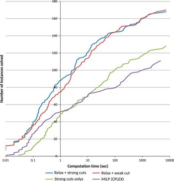
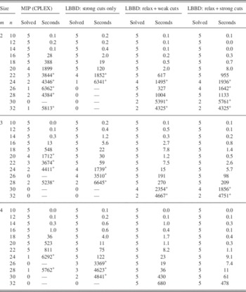
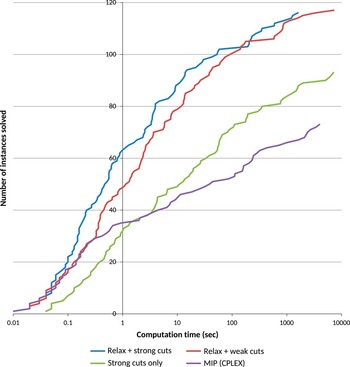
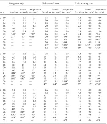
Table 1 shows our results for the ‘c’ instances. LBBD is clearly superior to MIP, running at least 1000 times faster on the larger instances with more than two resources. The advantage is less pronounced when there are only two resources, which is not surprising because there is less decoupling of the subproblem. The superiority of LBBD is equally evident in the performance profile of Figure 1.
Performance profile for all 180 ‘c’ instances

Computational results for the ‘c’ instances, which are designed to be difficult for logic-based Benders decomposition (LBBD)

n Tasks are scheduled on m resources. The number of problem instances solved (out of five) and average computation time in seconds are shown. Results are shown for the CPLEX mixed integer programming (MIP) solver, LBBD with strengthened cuts but no subproblem relaxation in the master problem, LBBD with a relaxation and simple nogood cuts, and LBBD with a relaxation and strengthened cuts.
+Computation terminated after 7200 seconds for instances not solved to optimality. In cases where CPLEX terminated prematurely due to lack of memory, the computation time was set at 7200 seconds when computing the average time for CPLEX.
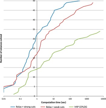
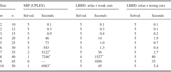
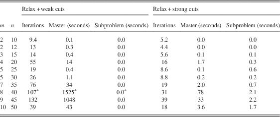
The superiority of LBBD is even clearer for the ‘e’ instances, as revealed in Table 2 and the performance profile in Figure 2.
Performance profile for all 50 ‘e’ instances. MIP=mixed integer programming

Computational results for the ‘e’ instances

LBBD=logic-based Benders decomposition; MIP=mixed integer programming.
+Computation terminated after 7200 seconds for instances not solved to optimality.
The importance of the subproblem relaxation is equally evident in the results. If strengthened nogood cuts are used without a relaxation, the advantage of LBBD is substantially reduced, and it disappears completely in some instances.
Strengthening of the nogood cuts, however, is not always effective. It actually worsens performance in ‘c’ instances with two resources, and it brings rather limited improvement in the overall performance profile. Even when the instances with two resources are removed from the profile, as in Figure 3, the effect of strengthening is not as great as one might expect. On the other hand, cut strengthening is significantly more effective in the ‘e’ instances, as is evident in Figure 2.
Performance profile for the 120 ‘c’ instances with three and four resources. MIP=mixed integer programming

6 Analysis of results
More detailed computational data can shed light on the results described above. Tables 3 and 4 show the average number of iterations for each instance size, as well as a breakdown of the average solution times by master problem and subproblem.
Computational analysis of logic-based Benders decomposition for ‘c’ instances, showing the average number of iterations and the average computation time spent solving master problems and subproblems

+Computation terminated for unsolved instances after the total computation time reaches 7200 seconds.
Computational analysis of logic-based Benders decomposition for ‘e’ instances

+Computation terminated for unsolved instances after the total computation time reaches 7200 seconds.
We can immediately see the effect of the subproblem relaxation. The lack of a relaxation results in a dramatic increase in the number of iterations and therefore in the solution time. This is intuitively reasonable, because a Benders method in effect computes the projection of the feasible set onto the master problem variables. As more Benders cuts are added, the projection is more accurately described. Eventually, enough cuts are added to describe the projection completely, and the problem can be solved by solving only the master problem. It is impractical to generate so many cuts, however, and the effectiveness of the Benders method rests on the fact that cut generation is guided by interim solutions of the master problem. Cuts tend to be generated only in the vicinity of the optimal solution, and this is enough to solve the problem. A relaxation of the subproblem is useful because it more tightly circumscribes the projection from the start, so that many fewer cuts are necessary to chip away regions near the optimum that are not part of the projection.
The absence of a relaxation not only generates more iterations, but each iteration requires longer to solve. This is because more iterations produce more Benders cuts, which makes the master problem larger and harder to solve. The tables suggest that a successful application of the Benders method tends to result in well under 100 iterations. After this point, solution of the master bogs down, and the method tends to fail.
The results also reveal why the ‘c’ instances are harder for LBBD. Once the number of tasks reaches a certain point, the subproblem solution time explodes, even while the master problem solution time remains small. This point is reached earlier when there are fewer resources, indicating that the key factor is the average number of tasks per resource. In fact, the break point is about 10 tasks/resource. Due to the uneven loads, this places subtantially more than 10 tasks on the fastest resource, whereupon the CP problem becomes highly combinatorial, and solution time explodes. This phenomenon does not occur in the ‘e’ instances, where there are only five tasks per resource, and the resource loads are more evenly balanced.
From a broader perspective, the ‘c’ instances are less suitable for LBBD because the assignment problem is relatively easy when there are only two or three resources. Most of the combinatorial complexity is relegated to the scheduling subproblem, which can quickly become intractable as the instances scale up. In the ‘e’ instances, the assignment problem bears a more equal share of the combinatorial burden. Decomposition is more effective because the labor is more equally shared between master and subproblem.
It is less obvious how the effect of cut strengthening can be explained, but a pattern is visible. We first observe that strong cuts tend to result in greater subproblem solution time per iteration, because the subproblem is solved repeatedly in each iteration to tighten the cuts. However, this tends to be more than offset by the smaller number of iterations. As one might expect, stronger cuts remove more solutions that lie outside the projection, and fewer cuts are therefore necessary. The key observation is that when there are fewer resources relative to tasks, the subproblem relaxation already substantially reduces the number of iterations. This means that there is less room for further reduction due to strong cuts. This is particularly evident in the ‘c’ instances with only two or three resources (Table 3).
The data further suggest that cut generation should result in a rough balance between the total master solution time and the total subproblem solution time. This is particularly evident for the ‘e’ instances (Table 4), for which weak cuts result in nearly 0 subproblem solution time, while strong cuts roughly equalize the master and subproblem time in most cases. LBBD is somewhat less efficient for instances with eight and nine resources, for which the master solution time is significantly greater than the subproblem time. This suggests that one should invest more time to generate stronger cuts for these instances.
7 Conclusions
Based on the experiments described above, we conclude that LBBD is more effective when the problem in fact decomposes. The planning and scheduling components should both embody substantial shares of the problem’s combinatorial complexity.
When the planning portion involves the assignment of tasks to resources, the average number of tasks per resource should be small enough that the assignment problem is roughly as hard as the scheduling problem. In particular, it should remain below the threshold at which solution time of the scheduling problem tends to explode. LBBD failure most often occurs when the CP solver blows up because of too many tasks are assigned to the resource. This is less likely to occur when no resource is significantly faster than others.
We also find that the most effective technique for reducing solution time is to include a relaxation of the subproblem in the master problem. This can dramatically reduce the number of iterations, as well as the solution time per iteration, because the master problems are smaller when there are fewer iterations.
The identification of stronger cuts can also significantly reduce the number of iterations, especially when the master and subproblem complexity are properly balanced. A rough guideline is to invest greater time in identifying strong cuts when the subproblem solution time per Benders iteration is less than the master problem solution time.
In any event, LBBD remains substantially faster than state-of-the art MIP on the problem class studied here. This is despite the marked improvement of MIP solvers, already highly advanced, over the last few years. The advantage exceeds a factor of 1000 for larger instances. In fact, the LBBD method presented here is best conceived as an enhancement of MIP rather than a competitor, because MIP solves the master problem, and LBBD will therefore improve as MIP improves. LBBD also benefits from advancements in CP, used here to solve the subproblem.
On the other hand, LBBD is likely to fail when the imbalance or size of the master and subproblem result in more than 100 Benders iterations.
These results suggest several research directions. When the number of tasks per resource crosses the CP solver’s tractability threshold, one option is to solve the scheduling subproblem with failure-directed search, which was recently introduced in the IBM CP optimizer. Another option is to decompose the scheduling problem itself using LBBD. This can be done by dividing the time horizon into segments and creating a subproblem for each segment. This approach has been successfully applied in the context of single-resource scheduling (Çoban & Hooker, Reference Çoban and Hooker2013).
The overriding importance of a subproblem relaxation suggests that further research should be conducted in this area. For example, some of the subproblem constraints could be incorporated verbatim into the master problem, along with the subproblem variables that occur within them. Normally, subproblem variables do not occur in the master, but their inclusion is consistent with the Benders mechanism so long as their solution values in the master are discarded before the next subproblem is solved. Their presence in the master serves only to restrict the possible values of the master variables. This strategy has been applied in a Benders-based solution of the home health-care delivery problem (Ciré & Hooker, Reference Ciré and Hooker2012). A practice of decomposing problems while allowing the components to intermingle could lead to a research program that improves decomposition methods in general.
One characteristic of LBBD not exploited here is that the subproblem is easily parallelized by assignining each facility to a different processor. This could be a significant advantage if there are a large number of facilities, or if the scheduling subproblem is itself decomposed.
Finally, the generation of strong Benders cuts could benefit from access to dual information in the subproblem solver. That is, the solver should report how it proved optimality or infeasibility. The cuts used here were strengthened by repeatedly re-solving the subproblem to tease out dual information, but cuts based on the actual dual solution could be much more effective.