1. Introduction
An axial compressor consisting of rows of rotors and stators uses the lift on the blades to increase the pressure of the through flow. As the flow is throttled at a fixed rotor speed, the angle of attack (AoA) on the rotor blades is raised, resulting in increased blade lift and thus higher pressure rise of the compressor. So, the compressor performance can be described by the pressure rise as a function of flow rate, namely a pressure rise characteristic. Generally, the characteristic curve will continue to rise with decreasing flow rate, provided that the flow remains circumferentially uniform. However, axisymmetric flow in the compressor will become unstable as the flow rate is reduced to a limit. Then, one to several cells of stalled flow develop over the compressor annulus, rotating in the direction of rotor rotation (Emmons, Kronauer & Rockett Reference Emmons, Kronauer and Rockett1959; Greitzer Reference Greitzer1976; Day Reference Day2016). Once it occurs, rotating stall will cause a severe degeneration in the performance of the compressor, limiting its useful operating range.
How does a compressor make the transition from a nominally steady, axisymmetric flow to rotating stall? This problem has been of great interest. Regarding this, the prediction of linear stability models, notably the Moore–Greitzer (Reference Moore and Greitzer1986) model, is that rotating stall grows from a type of long-length-scale disturbance, known as modal waves, whose primary mode has a wavelength as long as the compressor circumference. Similar to the classical Kelvin–Helmholtz and Tollmien–Schlichting instability waves, modal waves are sinusoidal and grow exponentially with time. Hoewver, the growth rate of this type of disturbance is generally low, such that the transition time from the onset of instability to fully developed stall is up to dozens or hundreds of rotor revolutions (typical time scale of modal-type inception). Also, its propagation speed is generally below 50 % of the rotor speed. The existence and features of modal waves were experimentally confirmed in the early 1990s (Mcdougall, Cumpsty & Hynes Reference Mcdougall, Cumpsty and Hynes1990; Garnier, Epstein & Greitzer Reference Garnier, Epstein and Greitzer1991); since then, the focus of rotating stall study has begun to shift from fully developed stall to the process of stall inception.
However, modal-type inception is not the only route to rotating stall. The use of improved instrumentation led to the discovery of another type of stall inception in experiments in the 1990s (Day Reference Day1993 a), termed as spike-type inception because of the spike-like appearance of the disturbances. Spikes are localised over just several blade spacings or pitches, typically an order of magnitude shorter in length scale than modal waves (Tan et al. Reference Tan, Day, Morris and WADIA2010). Correspondingly, this type of disturbance propagates faster and grows more rapidly, with a characteristic time scale of only several rotor revolutions. Moreover, the so-called ‘zero slope criterion’ (linear models predict that instability will occur when the compressor characteristic reaches the peak with zero slope, which is valid for modal waves) does not apply to spikes, for they tend to emerge when the characteristic seems to still be rising. Based on this observation, Camp & Day (Reference Camp and Day1998) proposed an empirical criterion for spike stall inception: there exists a rotor critical incidence, if it is exceeded before the peak of the characteristic is reached, then spike stall inception will occur; otherwise, stall will be initiated by modal waves.
Different from modal-type stall inception, spike-type inception cannot be explained by conventional stability theory. So, it is a difficult problem to mathematically model this type of spike instability and give an in-depth mechanical description, for which considerable efforts have been made over the past decades.
From a practical point of view, the aim to study stall inception is to develop an effective means to prevent or delay the onset of rotating stall in compressors. Based on linear stability models, stabilisation of a compression system has been realised either by controlling the unstable modes with additional perturbations (Paduano Reference Paduano1992; Hynes, Hendricks & Epstein Reference Hynes, Hendricks and Epstein1994; Nie et al. Reference Nie, Xu, Cheng and Chen2002) or by altering the system eigenvalues by means of some special casing treatments (Sun et al. Reference Sun., Liu, Hou and Sun2013; Sun et al. Reference Sun, Sun, Liu, Yu and Wang2014a ,Reference Sun, Liu, Jin, Gui and Sun b ). However, in contrast to modal waves, spikes have the features of being abrupt and localised (broadband), which pose significant challenges for their control via either active cancellation or passive suppression strategies (Paduano, Greitzer & Epstein Reference Paduano, Greitzer and Epstein2001). Especially, there is a lack of theoretical basis for developing novel methods to control spike-type stall.
As early as in the 1950s, Emmons, Pearson & Grant (Reference Emmons, Pearson and Grant1955) gave a qualitative explanation of stall propagation, suggesting the possibility of evolution of rotating stall from a short length scale disturbance. As illustrated in figure 1 (generally attributed to Emmons, also see Iura & Rannie Reference Iura and Rannie1954), if a minor flow non-uniformity causes flow separation on one blade in a highly loaded blade row, then the local blockage will divert the approaching flow such that the incidence angle is increased to the right of the stalled blade and decreased to the left. So, the next blade to the right will subsequently stall and the blade already stalled tends to unstall. Thus, a localised stall cell will be formed and propagate forward. Obviously, such a stall cell, which affects the flow around just a few aerofoils, is literally a spike which immediately disrupts the circumferential symmetry of the flow field. However, there is a lack of a mathematical model to support this stalling–unstalling scenario; even the model of Emmons et al. in the same paper was in favour of modal-type inception.
Physical mechanism for stall propagation in a cascade. Stall cell moves in the direction opposite to the blade movement in the reference fame fixed to the cascade.

Since approximately 2000, there has been an increasing trend to develop CFD (computational fluid dynamics) models to investigate the problem of spike-type stall inception. Much attention has been paid to what blade-passage-level flow structures/events are responsible for spike formation. Two different conceptual pictures of spike flow structure have been put forward, attracting wide interest. The first is forward spillage of tip-leakage flow at the blade’s leading edge and simultaneous backflow at the trailing edge, which were proposed as two criteria for spike formation (Vo, Tan & Greitzer Reference Vo, Tan and Greitzer2008). The second involves the radial vortex (also called tornado-like vortex) resulting from leading edge separation and its travelling from blade to blade (Yamada et al. Reference Yamada, Kikuta, Iwakiri, Furukawa and Gunjishima2013; Pullan et al. Reference Pullan, Young, Day, Greitzer and Spakovszky2015). The connection of radial vortices with spikes was initially suggested by Inoue et al. (Reference Inoue, Kuroumaru, Tanino and Furukawa2000, Reference Inoue, Kuroumaru, Yoshida and Furukawa2002) based on their detailed experiment for part-span stall cells (which are stable and can be measured with a phase-locked technique). They argued that spikes resembled the small cells since both had similar length scale and propagation speed. In the radial vortex scenario, a spike is considered to consist of a low-pressure part from the vortex core and a high-pressure part resulting from the passage blockage (Pullan et al. Reference Pullan, Young, Day, Greitzer and Spakovszky2015). However, in some cases, simulations of compressor instabilities demonstrated the importance of tip leakage flow, but show no sign of radial vortices (Ju & Ning Reference Ju and Ning2014; Bousquet et al. Reference Bousquet, Binder, Rojda and Thacker2022). In contrast, in other cases, simulations with and without tip clearance captured radial vortices during stall onset, indicating that spike formation does not depend on tip leakage (Pullan et al. Reference Pullan, Young, Day, Greitzer and Spakovszky2015). In addition, Hewkin-Smith et al. (Reference Hewkin-Smith, Pullan, Grimshaw, Greitzer and Spakovszky2019) suggested that the two flow events could act synergistically, with tip leakage flow being the cause of the high incidence necessary for the creation of radial vortices. In a special attempt, Gong et al. (Reference Gong, Tan, Gordon and Greitzer1999) developed a simplified CFD model that assumed an infinite number of blades and used a body force field to model the blade row effects. It was shown that the experimentally observed spike features could be reproduced, even if flow details at the blade-passage level were smeared out.
So, ‘at present, we do not have a description of stall cell formation which is acceptable to all’. We believe this comment made by Day (Reference Day2016) nearly 10 years ago still holds true.
This background motivates us to develop a new approach and focus on the problem of how nonlinearity causes the formation of spikes. So far, there is still a lack of insight into this basic problem, although it is generally recognised that spikes are nonlinear in nature. The CFD models naturally incorporated nonlinear effects through solving flow governing equations, but they did not explain how nonlinearity plays its role in a spike-type instability in much detail. Conventionally, in stability analysis, nonlinearity is associated with large disturbances. For instance, this notion is reflected in the computational model of Gong et al. (Reference Gong, Tan, Gordon and Greitzer1999), which used large input disturbances to trigger stall in the simulations (we will further discuss this in § 4.3). However, stall inception is a self-excited process. In practice, a compressor is usually throttled to a flow limit and then left to stall of its own accord. Hence, for spike stall to occur spontaneously, nonlinearity must set in from the very beginning when disturbances are still small or the blade row flow is almost circumferentially symmetrical, rather than arising from large disturbances. That is to say, if a compressor stalls via spikes, then it should represent such a flow system that cannot be linearised even to small perturbations.
Considering an individual blade row, since both upstream and downstream flows can be linearised to small perturbations, whether the flow system can be linearised or not depends on how flow separation develops inside the blade row. If flow separation develops gradually like the wall separation in a diffuser, then the blade row flow can be represented by a smooth characteristic, such as the well-used S-shaped curve in current rotating stall models (Koff & Greitzer Reference Koff and Greitzer1986). As such, linearising the upstream and downstream flow as well as the blade row characteristic must lead to an eigenvalue problem for describing the system dynamical behaviour, with each complex eigenvalue
 $\omega _{n}$
corresponding to a modal wave with the time dependence of
 $\mathrm{e}^{i{\omega _{n}}t}$
. Once there is a mode with a negative damping
 $\mathrm{Im}(\omega _{n})$
, it will grow exponentially in time, causing the system to lose stability; this is the modal route to rotating stall. For this route, nonlinear effects become significant only when the unstable mode grows to be sufficiently large, and their role is to limit its exponential growth (Moore Reference Moore1984, part III; Moore & Greitzer Reference Moore and Greitzer1986). In contrast, spike-type inception represents a kind of flow instability without eigenvalues. Behind the differences in phenomena (as mentioned previously), this is, in essence, the distinction between the two types of stall inception.
This leads us to deduce that, for a blade row under the condition of high incidence, it is possible for a sudden breakdown of attached flow to occur on some overloaded blade(s), causing a sharp drop in local pressure rise, so that local blade row characteristics can be approximately or ideally described by a discontinuous function. This situation may be analogous to the leading edge stall of an isolated aerofoil. In figure 2, leading edge stall is compared with two other common types of stall – trailing edge and thin aerofoil stalls (McCullough & Gault Reference Mccullough and Gault1951; van den Berg Reference Van den Berg1969). For leading edge stall, the lift coefficient suddenly drops from where the slope is still positive as the angle of attack
 $\alpha$
exceeds a critical value
 $\alpha _{cr}$
, rather than decreasing from the zero-slope peak as seen for the other two types of stall. That stall occurs at the zero-slope peak indicates that flow separation gradually develops on the aerofoil, whereas the ‘unexpected’ stalling prior to zero slope results from an abrupt flow separation over the suction surface.
Lift coefficient
 $C_{L}$
versus angle of attack
 $\alpha$
for an isolated aerofoil (after van den Berg Reference Van den Berg1969), with critical AoA
 $\alpha _{cr}$
corresponding to the maximum lift: (a) trailing edge stall; (b) leading edge stall; (c) thin aerofoil stall.

Note the similarity between the critical incidence found by Camp & Day (Reference Camp and Day1998) for spike inception and the critical angle of attack in leading edge stall of an isolated aerofoil. Camp & Day’s critical incidence also occurs before the slope of the characteristic would become zero, indicative of abrupt flow separation on the blades. Furthermore, it was also proposed that the blade loading at which both the forward spillage and backflow criteria occurred corresponded to Camp & Day’s critical incidence (Vo et al. Reference Vo, Tan and Greitzer2008; Tan et al. Reference Tan, Day, Morris and WADIA2010). This implies that these criteria can also be signs of abrupt drop in blade loading. Moreover, there are accumulating experimental and numerical results showing that leading edge separation possibly occurs in the tip region of a cascade blade due to high incidence, giving rise to shedding of a radial vortex of large strength (Yamada et al. Reference Yamada, Kikuta, Iwakiri, Furukawa and Gunjishima2013; Pullan et al. Reference Pullan, Young, Day, Greitzer and Spakovszky2015). Then, at the same time, there must be a corresponding drop in blade circulation or lift in the tip region, satisfying Kelvin’s theorem. Indeed, as shown by casing pressure measurements (Yamada et al. Reference Yamada, Kikuta, Iwakiri, Furukawa and Gunjishima2013), as a radial vortex is shed from the leading edge of a blade, the peak suction near the leading edge considerably diminishes or collapses.
For a blade row having a discontinuous local characteristic and operating sufficiently close to the stall point, a small velocity defect in the incoming flow can cause a large drop in blade loading. As such, the flow system cannot be linearised in the vicinity of the stall point, precluding the possibility of modal-type stall inception. As far as we know, the implication of a discontinuous characteristic to the problem of stall inception has not been explored up to now.
In the present paper, a two-dimensional (2-D) point vortex model is established to study how a spike is formed and grows into rotating stall in a cascade of aerofoils or a blade row, which has the following ingredients: (i) the cascade is replaced by an array of bound vortices, and large-scale shed vortices from the blades are represented by point vortices; (ii) it assumes that the cascade has a discontinuous bound circulation versus flow incidence characteristic.
First, we will demonstrate with this model that the extreme nonlinearity associated with the discontinuous characteristic plays a key role in the spontaneous formation of spikes, or it is such nonlinearity that determines that the route to rotating stall is through spikes.
Moreover, we will use this model to elucidate the flow structure of spikes. Although CFD simulations have linked spikes with radial vortices or tip leakage flow, these flow structures have relatively fixed length scales (radial vortices are of sub-passage dimensions, while the tip leakage flow in the criteria of Vo et al. spans roughly two passages), which can hardly explain that the extent of a spike increases rapidly as it propagates. In other words, the previous depictions of spike flow structure may be incomplete, which need further improvements.
Finally, this simple model will be applied to capture and explain the key features of spike-type stall inception. Especially, we notice that no attempt has previously been made to predict the temporal variation of stall cell size and compare the results with existing experiments. Also, there is little detailed knowledge on how spikes grow with time, though it is expected that they would not grow exponentially like modal waves. We will provide new results and analysis in this regard.
Although our understanding of spike-type inception has considerably improved compared with when it was first discovered, many questions regarding its underlying mechanism remain unanswered. We will try to shed light on some of these key questions (as stated previously) from the perspective of vortex dynamics by the advantage of the point vortex model being simple to understand.
2. Formulation
As a powerful approach for modelling unsteady separated flow, vortex methods have been widely used to predict dynamic-stall or post-stall behaviour of an isolated aerofoil (Katz Reference Katz1981; Pullin & Wang Reference Pullin and Wang2004; Ramesh et. al. Reference Ramesh, Gopalarathnam, Granlund, M.V. and Edwards2014; Darakananda & Eldredge Reference Darakananda and Eldredge2019). However, there were very limited efforts to extend vortex methods to rotating stall occurring in a cascade of aerofoils. In only a few attempts, this kind of method was used to simulate fully developed rotating stall with some success (Stenning, Seidel & Senoo Reference Stenning, Seidel and Senoo1959; Spalart Reference Spalart1985).
Different from these previous efforts, the present vortex model focuses on the problem of stall inception. For simplification, a blade row is replaced by an array of bound vortices or, in other words, the blade loading is modelled by concentrated lift generated by the bound vortices (hereafter, we will use ‘blade’ and its replacement ‘bound vortex’ interchangeably). Also, as suggested by the experiment of Kriebel, Seidel & Schwind (Reference Kriebel, Seidel and Schwind1958), it is assumed that shed vorticity is concentrated in point vortices departing from the blades. So, in the present study, development of the flow instability will be described by the evolution of point vortices. Next, the formulation of this point vortex model will be presented in detail.
2.1. Velocity field
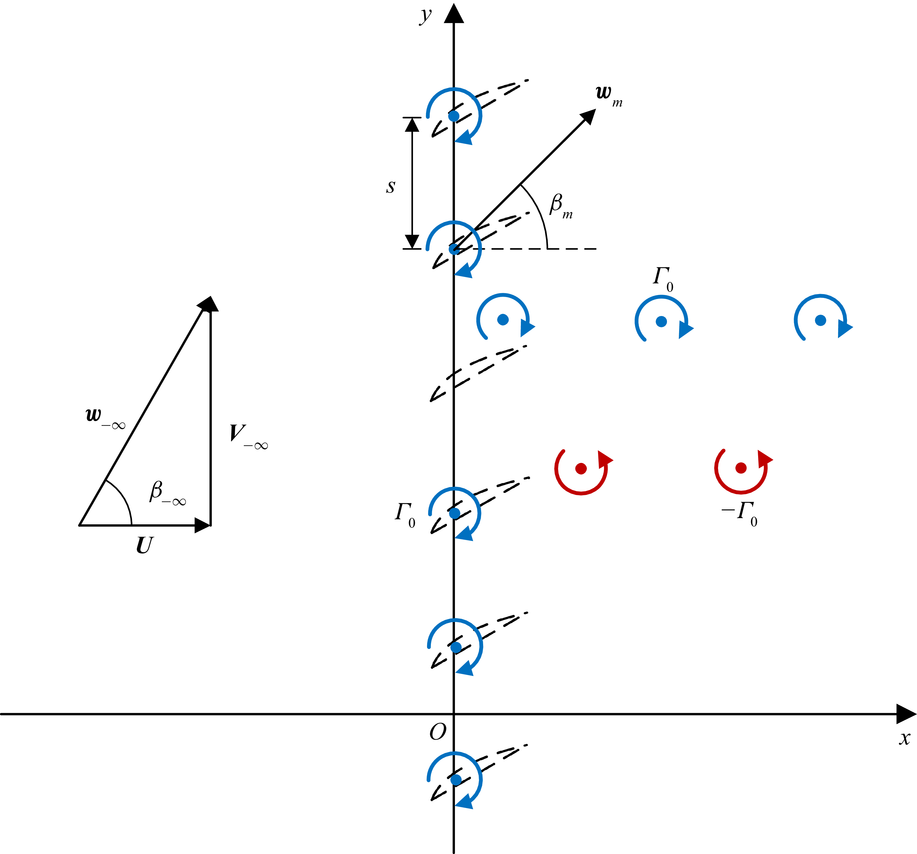
As illustrated in figure 3, an array of equidistant bound vortices lies along the y axis in the xy plane, which represents an unwrapped annular blade row of very high hub-to-tip ratio. So, 2-D flow is assumed in the present model. Previously it was speculated that spikes were due to three-dimensional (3-D) effects since they were usually observed to occur in the tip region of a rotor. However, as demonstrated by He (Reference He1997) and Pullan et al. (Reference Pullan, Young, Day, Greitzer and Spakovszky2015), 2-D CFD solvers were capable of simulating spike stall inception in a linear cascade. This provides evidence that 3-D effects are not a necessary requirement for spike formation. So, the reason why spikes tend to appear in the tip region is probably because excessive incidence more likely occurs in this region than in the lower regions of the blades. Also, compressibility and viscosity of the fluid are neglected as they are not essential factors to the flow instability problem.
Schematic of a cascade of blades (dashed lines) that are replaced by an array of bound vortices. Stall and starting vortices with circulations
 $\pm \varGamma _{0}$
are shed from the cascade and convect downstream.

The cascade flow is periodic in the y direction (circumferential direction) with a period of
 $2\pi\! R$
, where
 $R$
is the mean radius of the corresponding annular blade row. Let there be
 $N_{b}$
bound vortices within one period (i.e.
 $N_{b}$
is the number of blades). Then, the spacing between two adjacent bound vortices or blade pitch is
 $s=2\pi\! R/N_{b}$
. The positions of the blades are given as:
 $ y_{n}=(n-{1}/{2})s$
, where
 $n=1,2,\ldots ,N_{b}$
. So, through using bound vortices or point-like body forces to represent a blade row, the present model is able to take into account the effects of blade discreteness. This is different from the models relying on the assumption of infinite number of blades, such as actuator disk models (Emmons et al. Reference Emmons, Pearson and Grant1955; Marble Reference Marble1955; Sears Reference Sears1955; Stenning Reference Stenning1980; Moore Reference Moore1984; Moore & Greitzer Reference Moore and Greitzer1986) and the distributed body force model of Gong et al. (Reference Gong, Tan, Gordon and Greitzer1999).
In the absolute frame of reference, the blades move to the negative y direction at constant speed
 $V$
(wheel speed). When the reference frame is changed to that fixed to the cascade, in which the present model is set up, the incoming flow approaches the cascade with velocity
 $\boldsymbol{w}_{-\boldsymbol{\infty }}=(U,V_{-\infty })$
, as shown in figure 3. If the absolute velocity of the incoming flow is axial, then
 $V_{-\infty }=V$
; we assume this is the case throughout.
When the cascade is in steady operation, all the blades have the same circulation
 $\varGamma _{0}$
in the clockwise direction (negative sign). Once flow instability occurs, the bound circulations are no longer constant, varying with both time and location. Consequently, there will be vorticity shed from the cascade into the ambient fluid, which is in the form of point vortices. When a blade suddenly stalls, it will shed a stall vortex with strength being equal to the drop in its bound circulation. Subsequently, when it unstalls, that blade will shed a starting vortex of equal but opposite strength. Further discussion of the vortex shedding will be continued in §§ 2.2 and 2.4. As time proceeds, there will appear increasingly more shed vortices moving in the flow field, interacting with each other and with the bound vortices, as illustrated in figure 3. However, the total circulation in the flow field is conserved all the time,
 $\varGamma _{t}=N_{b}\varGamma _{0}$
, in accordance with Kelvin’s theorem.
Throughout the paper, the annular blade row radius R and the wheel speed
 $V$
are selected as the reference length and velocity, respectively. So, time is normalised by
 $R/V$
, pressure by
 $\rho V^{2}$
(
 $\rho$
is the fluid density), and both circulation and velocity potential by
 $\textit{VR}$
.
Note that each point vortex, either bound or shed, has an infinite number of ‘images’ because periodic boundary conditions are imposed on
 $y=0$
and
 $2\pi\! R$
. A point vortex and its images constitute an infinite row of point vortices, for which the complex potential at time
 $t$
is expressed as follows (Lamb Reference Lamb1932):
 \begin{equation}F_{m}(z,t)=\frac{\varGamma _{m}(t)}{2\pi \mathrm{i}}\ln \left\{\sinh \left[\frac{1}{2}\left(z-z_{m}(t)\right)\right]\right\}\! ,\end{equation}
where
 $z=x+\mathrm{i}y$
with
 $\mathrm{i}=\sqrt{-1} ; \varGamma _{m}$
and
 $z_{m}$
denote the instantaneous circulation and position of the mth point vortex (
 $z_{m}$
is fixed for a bound vortex), respectively. Notice that during the process that a blade is shedding a vortex, both its bound circulation and the strength of the new shed vortex are time dependent, for which details will be presented in the next section. So, the derivative of (2.1) gives the induced velocity of the mth point vortex,
 \begin{align} u_{m}(x,y,t) & =-\frac{1}{4\pi }\frac{\varGamma _{m}(t)\sin \left(y-y_{m}(t)\right)}{\cosh \left(x-x_{m}(t)\right)-\cos \left(y-y_{m}(t)\right)} ,\\[-8pt]\nonumber\end{align}
 \begin{align} v_{m}(x,y,t) & =\frac{1}{4\pi }\frac{\varGamma _{m}(t)\sinh \left(x-x_{m}(t)\right)}{\cosh \left(x-x_{m}(t)\right)-\cos \left(y-y_{m}(t)\right)} .\end{align}
With all the point vortices being superimposed with the uniform incoming flow, the complex potential is written as
 \begin{equation}F(z,t)=\left[U-\mathrm{i}\left(V_{-\infty }+\frac{\varGamma _{0}}{2s}\right)\right]z+\frac{1}{2\pi \mathrm{i}}\sum _{m=1}^{N_{t}}\varGamma _{m}(t)\ln \left\{\sinh \left[\frac{1}{2}\left(z-z_{m}(t)\right)\right]\right\}\! ,\end{equation}
where
 $ N_{t}$
is the total number of point vortices at time
 $t$
, including both bound and shed vortices. Accordingly, the flow velocity is given by
 \begin{align} u(x,y,t) & =U-\frac{1}{4\pi }\sum _{m=1}^{N_{t}}\frac{\varGamma _{m}(t)\sin \left(y-y_{m}(t)\right)}{\cosh \left(x-x_{m}(t)\right)-\cos \left(y-y_{m}(t)\right)} ,\\[-8pt]\nonumber\end{align}
 \begin{align} v(x,y,t) & =V_{-\infty }+\frac{\varGamma _{0}}{2s}+\frac{1}{4\pi }\sum _{m=1}^{N_{t}}\frac{\varGamma _{m}(t)\sinh \left(x-x_{m}(t)\right)}{\cosh \left(x-x_{m}(t)\right)-\cos \left(y-y_{m}(t)\right)} .\end{align}
It can be easily verified that, as
 $x\rightarrow -\infty$
, the above-mentioned equations meet the upstream boundary condition.
2.2. Generation and advection of shed vortices
Evidently, a certain time is required for shed vorticity to accumulate near the separation point before a stall or a starting vortex is completely formed. This short time, denoted by
 $\tau _{d}$
, is referred to as boundary layer delay (Kriebel et al. Reference Kriebel, Seidel and Schwind1958; Stenning Reference Stenning1980) or blade response time (Hynes et al. Reference Hynes, Hendricks and Epstein1994), which characterises the time scale for the adjustment of blade loading after a sudden change in incidence. In this model, the rolling-up vortex sheet that is being shed from a blade is replaced by a point vortex (nascent vortex) and a feeding sheet of vorticity joining it to the blade, as illustrated in figure 4 (figure 4
a is similar to figure 1, but here it is emphasised that a localised stall cell emerges as the result of abrupt leading edge stall rather than the gradual separation over the blade suction surface; more discussion of this will be given later). During the vortex shedding process, circulation is continuously fed into the nascent vortex through the feeding sheet. This idea was first proposed by Brown & Michael (Reference Brown and Michael1954) for analysing steady separated flow over a delta wing and, since then, has been extended to the problems of unsteady vortex shedding (Rott Reference Rott1956), unsteady vortex lift (Wang & Eldredge Reference Wang and Eldredge2013) and vortex sound interaction (Howe Reference Howe1996; Kuo & Dowling Reference Kuo and Dowling2000; Dai, Jing & Sun Reference Dai, Jing and Sun2011).
Illustration of the vortex shedding process: (a) physically, the shear layer shed from a blade rolls up into a growing spiral vortex; (b) in this model, the spiral is replaced by a variable-strength point vortex and a feeding sheet of vorticity.

Because its strength depends on time, a nascent vortex must move at a velocity departing from local flow velocity, such that the Joukowski lift
 $\boldsymbol{F}_{\!\boldsymbol{L}}$
on it balances the pressure jump
 $p_{+}-p_{-}$
across the feeding sheet. Hence, the vector coordinate
 $\boldsymbol{r}_{\!\boldsymbol{n}}=(x_{n},y_{n})$
of a shed vortex
 $\varGamma _{n}$
during its formation phase satisfies the following equation (Rott Reference Rott1956):
 \begin{equation}\frac{\mathrm{d}\boldsymbol{r}_{\!\boldsymbol{n}}}{\mathrm{d}t}=\boldsymbol{w}\left(\boldsymbol{r}_{\!\boldsymbol{n}},t\right)-\frac{\boldsymbol{r}_{\!\boldsymbol{n}}-\boldsymbol{r}_{\mathbf{0}\boldsymbol{n}}}{\varGamma _{n}}\frac{\mathrm{d}\varGamma _{n}}{\mathrm{d}t},\end{equation}
where
 $\boldsymbol{w}=(u,v)$
is the local flow velocity at
 $(x_{n},y_{n})$
, given in (2.4) (excluding the contribution from
 $\varGamma _{n}$
itself); and
 $\boldsymbol{r}_{\mathbf{0}\boldsymbol{n}}$
denotes the location of the blade releasing the nascent vortex.
For the present simplified model, it needs as an input the nascent vortex circulation as a function of time. However, there is a lack of such information in the open literature for stalling aerofoils in a cascade. Perhaps the most relevant results are those obtained for leading edge vortices (LEVs) over an isolated pitching wing. It was shown by experiments that the LEV circulation exhibited a roughly linear growth with time, followed by a transition to a constant value (Otomo et al. Reference Otomo, Henne, Mulleners, Ramesh and Viola2021). In light of this, the following relation is assumed for the time dependence of
 $\varGamma _{n}$
:
 \begin{equation}\varGamma _{n}\left(t\right)=\pm \varGamma _{0}\times \begin{cases} 1.2\dfrac{t}{\tau _{d}} \quad \quad\quad \quad\quad\quad \quad\; \left(0\leq t\leq \dfrac{2}{3}\tau _{d}\right)\!, \\[9pt] 1-1.8\!\left(1-\dfrac{t}{\tau _{d}}\right)^{2} \quad \quad \left(\dfrac{2}{3}\tau _{d}\lt t\leq \tau _{d}\right)\!, \\ \end{cases} \end{equation}
where the plus or minus sign corresponds to a stall or starting vortex, respectively; and
 $t$
is measured relative to the beginning time of the vortex shedding process. As seen in figure 5, the (2.6) fits well with the measurements from Otomo et al. (figure 16a in their paper). We have digitised the data from the published figure, but the data density is reduced to some extent.
Magnitude of shed vortex circulation as a function of time, where circular symbols are the data of Otomo et al. (Reference Otomo, Henne, Mulleners, Ramesh and Viola2021), the solid line represents (2.6).

Following Hynes et al. (Reference Hynes, Hendricks and Epstein1994), the boundary layer delay
 $\tau _{d}$
is estimated by 1.5 times of the blade passage convection time,
 \begin{equation}\tau _{d}=1.5\frac{c_{x}}{U},\end{equation}
where
 $c_{x}=c\cos \gamma$
is the axial chord length, with
 $c$
and
 $\gamma$
being the chord length and stagger angle of blades, respectively. It is worth mentioning that
 $c_{x}$
is the only blade geometrical parameter adopted in this model, and it is only used to estimate the boundary layer delay.
Special care is needed to determine the initial velocity of a nascent vortex, since the second term in the right-hand side of (2.5) becomes singular when
 $\varGamma _{n}=0$
at
 $t=0$
. However, this term can be rewritten as
 $(-({\boldsymbol{r}_{\!\boldsymbol{n}}-\boldsymbol{r}_{\mathbf{0}\boldsymbol{n}}})/{\varGamma _{n}})( {\mathrm{d}\varGamma _{n}}/{\mathrm{d}t})= -({\boldsymbol{r}_{\!\boldsymbol{n}}-\boldsymbol{r}_{\mathbf{0}\boldsymbol{n}}})/{t}\rightarrow - {\mathrm{d}\boldsymbol{r}_{\!\boldsymbol{n}}}/{\mathrm{d}t}$
as
 $t\rightarrow 0$
. So, there is the result of
 ${\mathrm{d}\boldsymbol{r}_{\!\boldsymbol{n}}}/{\mathrm{d}t}=\boldsymbol{w}(\boldsymbol{r}_{\!\boldsymbol{n}},0)/{2}$
at the initial instant.
When
 $t\gt \tau _{d}$
, the circulation
 $\varGamma _{n}$
becomes constant since there is no feeding of vorticity any longer. Then, (2.5) reduces to
 \begin{equation}\frac{\mathrm{d}\boldsymbol{r}_{\!\boldsymbol{n}}}{\mathrm{d}t}=\boldsymbol{w}(\boldsymbol{r}_{\!\boldsymbol{n}},t) .\end{equation}
That is to say that a free vortex of constant strength just convects at the local flow velocity.
The initial conditions for (2.5) are
 $\boldsymbol{r}_{\!\boldsymbol{n}}=\boldsymbol{r}_{\mathbf{0}\boldsymbol{n}}$
when
 $t=t_{0n}$
(
 $t_{0n}$
denotes the time when the nascent vortex begins to shed). The trajectories of the shed vortices can be calculated by numerically integrating (2.5). By tracking all the vortices moving in the flow field, the vorticity distribution,
 $\sum \varGamma _{n}\delta (x-x_{n})\delta (y-y_{n})$
, is obtained at any time
 $t$
, where the summation is over every shed and bound vortex. Then, all the other time-dependent flow variables can be determined for the unsteady potential flow.
2.3. Pressure equation
Time-dependent pressure is calculated by using the unsteady Bernoulli equation. To do this, each shed vortex
 $\varGamma _{n}$
is paired with another vortex of equal but opposite strength,
 $\varGamma _{n}^{*}$
, located at the blade from which
 $\varGamma _{n}$
is released. So, letting
 $\varGamma _{n}$
be released from the mth blade at
 $z_{m}$
, whose current circulation is
 $\varGamma _{m}$
, there is the following relation:
 \begin{equation}\varGamma _{m}=\varGamma _{0}-\sum _{z_{n}^{*}=z_{m}}\varGamma _{n} .\end{equation}
Notice that the subscript m only refers to blades or bound vortices for the moment. Equation (2.9) states nothing but the conservation of circulation, namely that the current circulation of a blade is equal to the initial circulation
 $\varGamma _{0}$
deducting the sum of the circulations shed from that same blade. So, (2.3) for the complex potential can be rewritten as
 \begin{align}F & =\left[U-\mathrm{i}\left(V_{-\infty }+\frac{\varGamma _{0}}{2s}\right)\right]z +\frac{1}{2\pi \mathrm{i}}\sum _{m=1}^{N_{b}}\left(\varGamma _{m}+\sum _{z_{n}^{*}=z_{m}}\varGamma _{n}\right)\ln \left\{\sinh \left[\frac{1}{2}\left(z-z_{m}\right)\right]\right\}\nonumber\\& \quad +\frac{1}{2\pi \mathrm{i}}\sum _{n}\varGamma _{n}\ln \frac{\sinh \left[\frac{1}{2}\left(z-z_{n}\right)\right]}{\sinh \left[\frac{1}{2}\left(z-z_{n}^{*}\right)\right]},\end{align}
where the summation in the last term is over all the shed vortices, including the nascent vortices. By substituting (2.9) into (2.10), and using the identity
 $\sin (Nz)=2^{N-1}\times \prod _{k=0}^{N-1}\sin (z+{k\pi }/{N})$
(Gradshteyn & Ryzhikis Reference Gradshteyn and Ryzhik2007), we get
 \begin{align} F & =\left[U-\mathrm{i}\left(V_{-\infty }+\frac{\varGamma _{0}}{2s}\right)\right]z+\frac{\varGamma _{0}}{2\pi \mathrm{i}}\ln \left\{\sinh \left[\frac{\pi }{s}\left(z-z_{0}\right)\right]\right\}\nonumber\\[5pt]& \quad +\frac{1}{2\pi \mathrm{i}}\sum _{n}\varGamma _{n}\ln \frac{\sinh \left[\frac{1}{2}\left(z-z_{n}\right)\right]}{\sinh \left[\frac{1}{2}\left(z-z_{n}^{*}\right)\right]},\end{align}
where
 $z_{0}$
is the position of the bound vortex nearest to the coordinate origin. This states that the complex potential at any time can be decomposed into two parts: the steady-state potential before vortex shedding and that part due to the vortex pairs each of which consists of
 $\varGamma _{n}$
at
 $z_{n}$
and
 $\varGamma _{n}^{*}$
at
 $z_{n}^{*}$
. In (2.11), only the last term on its right-hand side is time-dependent, so the time derivative of the complex potential is
 \begin{equation}\frac{\partial F}{\partial t}=\frac{1}{2\pi \mathrm{i}}\sum _{\nu }\dot{\varGamma }_{\nu }\ln \frac{\sinh \left[\frac{1}{2}\left(z-z_{\nu }\right)\right]}{\sinh \left[\frac{1}{2}\left(z-z_{\nu }^{*}\right)\right]}-\sum _{n}\left(u_{n}-\mathrm{i}v_{n}\right)\left(\dot{x}_{n}+\mathrm{i}\dot{y}_{n}\right)\!,\end{equation}
where
 $\dot{\varGamma }_{\nu }$
is the time rate of change of circulation for each nascent vortex (denoted by subscript
 $\nu$
);
 $(u_{n},v_{n})$
is the induced velocity of the nth shed vortex, given by (2.2), while
 $(\dot{x}_{n},\dot{y}_{n})$
is its convection velocity, given in (2.5).
The flow field upstream of the cascade is almost free of vorticity, since the shed vortices are mainly convected downstream with the mean flow. So, it is appropriate to apply the unsteady Bernoulli equation between an upstream observation point and far upstream,
 \begin{equation}p+\frac{1}{2}\big(u^{2}+v^{2}\big)+{Re}\left(\frac{\partial F}{\partial t}\right)=p_{-\infty }+\frac{1}{2}\big(U^{2}+V_{-\infty }^{2}\big)+\textit{Re}\left(\frac{\partial F_{-\infty }}{\partial t}\right)\!.\end{equation}
As
 $x\rightarrow -\infty$
,
 $\ln ({\sinh [({1}/{2})(z-z_{\nu })]}/{\sinh [({1}/{2})(z-z_{\nu }^{*})]})=(z_{\nu }-z_{\nu }^{*})/{2}$
and
 $u_{n}-\mathrm{i}v_{n}=-\varGamma_{n}/(4\pi\mathrm{i})$
, there is the asymptotic result,
 \begin{equation}\frac{\partial F_{-\infty }}{\partial t}=\frac{1}{4\pi \mathrm{i}}\left[\sum _{\nu }\dot{\varGamma }_{\nu }\left(z_{\nu }-z_{\nu }^{*}\right)+\sum _{n}\varGamma _{n}\left(\dot{x}_{n}+\mathrm{i}\dot{y}_{n}\right)\right]\!.\end{equation}
Substituting into (2.13) the time derivatives of the complex potential from (2.12) and (2.14), we arrive at the following equation:
 \begin{align}p-p_{-\infty } & =\frac{1}{2}\big(U^{2}+V_{-\infty }^{2}-u^{2}-v^{2}\big)-\sum _{\nu }\dot{\varGamma }_{\nu }\left[\varphi _{\nu }-\frac{1}{4\pi }\left(y_{\nu }-y_{\nu }^{*}\right)\right]\nonumber\\& \quad +\sum _{n}\left[u_{n}\dot{x}_{n}+\left(v_{n}+\frac{\varGamma _{n}}{4\pi }\right)\dot{y}_{n}\right]\!,\end{align}
where
 \begin{equation} \varphi _{\nu }=\mathrm{Re}\left\{\frac{1}{2\pi \mathrm{i}}\ln \frac{\sinh \left[\frac{1}{2}\left(z-z_{\nu }\right)\right]}{\sinh \left[\frac{1}{2}\left(z-z_{\nu }^{*}\right)\right]}\right\}\! . \end{equation}
The branch cut of the multivalued function
 $\varphi _{\nu }$
is as shown in figure 4, which can also be regarded as the feeding sheet of vorticity. When
 $(2.15)$
is used to solve for the unsteady pressure
 $p$
,
 $p_{-\infty }$
may be considered as the reference pressure and set to zero, because all the disturbances vanish in the far field.
2.4. Local cascade characteristic
It is necessary to specify a local cascade characteristic (blade characteristic) to close the formulation of the present model. Since the early study of rotating stall, it has been assumed that a compressor blade row can be analogous to paralleling channels. Koch (Reference Koch1981) further proposed that an analogy could be made between compressor and diffuser performance to obtain a correlation of stalling pressure rise coefficient versus cascade parameters. The diffuser analogy led to smooth characteristics commonly used in compressor stability analysis. However, as mentioned, a blade row can be more complicated in that flow separation is likely to occur on an overloaded blade in an abrupt manner. In particular, if leading edge separation occurs on a blade, it will give rise to a radial vortex (Inoue et al. Reference Inoue, Kuroumaru, Tanino and Furukawa2000, Reference Inoue, Kuroumaru, Yoshida and Furukawa2002; Yamada et al. Reference Yamada, Kikuta, Iwakiri, Furukawa and Gunjishima2013; Pullan et al. Reference Pullan, Young, Day, Greitzer and Spakovszky2015), so that the blade circulation is abruptly fed to the radial vortex. Hence, the resulting local characteristic should be very different from that due to the progressive build-up of passage blockage as occurs in diffusers.
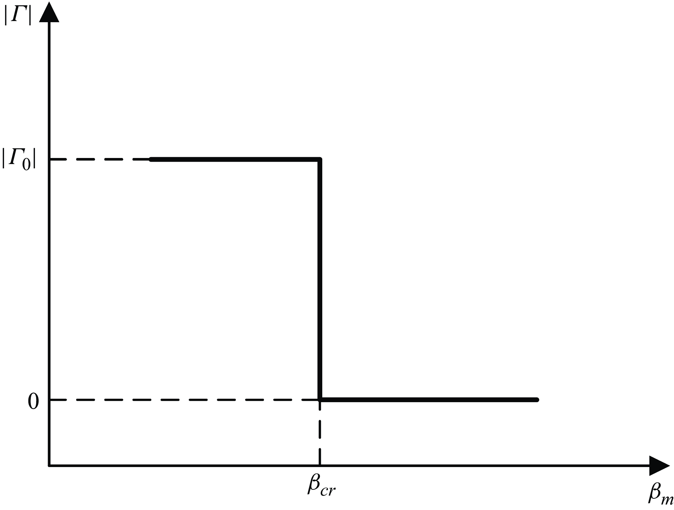
So, the following step-type blade characteristic is assumed:
 \begin{equation}\varGamma =\varGamma _{0}-\varGamma _{0}h\left(\beta _{m}-\beta _{cr}\right)\!,\end{equation}
where
 $\beta _{m}$
is local flow angle at the position of a blade (see figure 3),
 $\beta _{cr}$
is the critical angle at which leading edge separation occurs and
 $h(\beta )$
denotes the Heaviside function. This form of characteristic is shown in figure 6. Obviously, this represents an idealised situation (local pumping ability suddenly switches on and off), but the effects of abrupt change in blade loading are singled out in this way.
Local cascade characteristic (bound circulation versus flow angle) given by the Heaviside function.

Although it is well recognised that significant drop in blade loading occurs when blades stall, there is a lack of quantitative results on how much bound circulation is left on the stalled blades. Perhaps Kriebel et al. (Reference Kriebel, Seidel and Schwind1958) provided the only experimental results in this regard, which were obtained on a stationary circular cascade and showed that the pressure difference between the suction and pressure sides of the stalled blades almost vanished, i.e. nearly all of their bound circulation was lost. The experimental evidence is considered as a basis for (2.17).
It is also assumed that the blade stalling and unstalling starts at the same critical angle, i.e. the step-type characteristic is free of hysteresis. Based on Moore’s (Reference Moore1984, part I) idea of an underlying axisymmetric characteristic and its further development (Koff & Greitzer Reference Koff and Greitzer1986), it is common for rotating stall models to adopt single-valued or no-hysteresis characteristics. However, the model predictions are able to reproduce the stall/recovery hysteresis observed in experiments. So, this indicates that the hysteresis exhibited in the actual characteristics turns out to be a system feature that depends on the existence of rotating stall (Moore & Greitzer Reference Moore and Greitzer1986).
Equation (2.17) in combination with (2.6) for the time dependence of the shed circulation are used to describe the unsteady response of a blade. As local flow angle
 $\beta _{m}$
exceeds the critical angle
 $\beta _{cr}$
, a normal or unstalled blade immediately starts to shed vorticity, until all its circulation is transferred to the stall vortex after the time delay of
 $\tau _{d}$
. Conversely, as
 $\beta _{m}$
just decreases below
 $\beta _{cr}$
, a stalled blade starts to shed a starting vortex, so that its bound circulation is restored at the end of the time delay.
Although smooth characteristics have been commonly employed in existing rotating stall models, there were a few exceptions to be discussed in detail here. Marble (Reference Marble1955) first proposed a type of characteristic with a discontinuity at the stall point; and owing to this nonlinear characteristic, his model (which linearises both upstream and downstream flow) is perhaps the only small perturbation model that is able to predict the size of a stall cell, in addition to propagation speed. Stenning et al. (Reference Stenning, Seidel and Senoo1959) hypothesised a step-type characteristic with hysteresis for their vortex flow model, which calculated the properties of a full stall cell using an iterative algorithm. Moore (Reference Moore1984, Part III) simplified compressor characteristics as line-segment curves (with the step function being one special case) to facilitate solving the Lienard equation for stall oscillations in the phase space. His method found that rotating stall had the nature of a limit cycle.
All these previous studies concentrated on fully developed rotating stall. When the oscillation amplitude is large, as is the case of fully developed stall, the flow pattern depends on the entire unstable part of the characteristic, no matter whether this part is steep or not. Thus, the exact shape of this part may be unimportant (Koff & Greitzer Reference Koff and Greitzer1986). In contrast, for the inception process when disturbances are still small, the characteristic is essentially linear if the unstable part decreases smoothly, whereas it can be nonlinear if this part drops sharply. This difference is crucially important to the development of initial disturbances.
3. Method of calculation
3.1. Vortex core model
When a shed vortex is in the proximity of a bound vortex or another shed vortex, these vortices cannot be considered anymore as concentrated singularities of infinite vorticity, otherwise, they will induce unphysically large velocities on each other. So, as with other discrete vortex methods, a vortex core model is required to desingularise (2.2) for the induced velocity. Physically, as the shear layer shed from a blade rolls up, the tightly wound spiral will be smeared out by viscous diffusion into a vortex core with a smooth distribution of vorticity. Besides, because bound circulation is about a finite-chord blade rather than a singular point in reality, we also need to assign a finite core to the bound vortex that replaces the blade.
With a finite core of a small radius
 $\sigma _{m}$
being introduced to each point vortex, (2.2) is modified as
 \begin{equation}u_{m}=-\frac{\varGamma _{m}}{4\pi }\frac{\sin \left(y-y_{m}\right)}{\sqrt{\left[\cosh \left(x-x_{m}\right)-\cos \left(y-y_{m}\right)\right]^{2}+\left(\frac{\sqrt{2}}{2}\sigma _{m}\right)^{4}}} ,\end{equation}
 \begin{equation}v_{m}=\frac{\varGamma _{m}}{4\pi }\frac{\sinh \left(x-x_{m}\right)}{\sqrt{\left[\cosh \left(x-x_{m}\right)-\cos \left(y-y_{m}\right)\right]^{2}+\left(\frac{\sqrt{2}}{2}\sigma _{m}\right)^{4}}} .\end{equation}
For simplicity, the bound and shed vortices use the same vortex core model. The induced velocity is thus bounded with a maximum at the core edge, and vanishing at the core centre. For a point close to
 $(x_{m},y_{m})$
, (3.1a
,
b
) is reduced to
 $w_{\theta }=({\varGamma _{m}}/{2\pi })({r}/{\sqrt{r^{4}+\sigma _{m}^{4}}})$
(
 $w_{\theta }$
is the azimuthal velocity at distance
 $r$
from the vortex centre), which is referred to as the Vatistas model. This algebraic vortex core model, proposed by Vatistas, Kozel & Mih (Reference Vatistas, Kozel and Mih1991) as an empirical relation, is a close approximation to the Lamb–Oseen model which is an exact solution to the Navier–Stokes equations.
For a shed vortex, the vorticity in its core will diffuse outward as it is convected downstream. So, Bhagwat & Leishman (Reference Bhagwat and Leishman2002) proposed the following relation for the expansion of a vortex core:
 \begin{equation}\sigma _{n}=\sqrt{\sigma _{0}^{2}+aT_{n}} ,\end{equation}
where
 $\sigma _{0}$
is an initial core radius and
 $T_{n}$
is the age of the nth shed vortex; the diffusion coefficient
 $a=4\alpha \nu _{t}$
, with
 $\alpha =1.25643$
(Oseen parameter) and
 $\nu _{t}$
being the non-dimensional turbulent viscosity. However, (3.2) is based on the Lamb–Oseen model derived for an isolated vortex. When many vortices interact with each other strongly, turbulent diffusion may be further enhanced. So, Kuwahara & Takami (Reference Kuwahara and Takami1973) treated the viscosity for vortex core diffusion as a kind of ‘artificial viscosity’ with adjustable values in their discrete vortex model. Similarly,
 $a$
in (3.2) is considered as a smoothing parameter with a suitably chosen value. In the present calculations,
 $a=0.02$
is assumed throughout.
As for the bound vortices, their core size remains constant. For simplicity, it is also assumed that
 $\sigma _{0}$
of the shed vortices is the same as the core radius of the bound vortices, which is always specified to be
 $0.3s$
in the calculations.
3.2. Calculation procedure
Before the start of the calculation, a number of parameters need to be specified, which are: the number of blades
 $N_{b}$
, upstream axial velocity
 $U$
, initial bound circulation
 $\varGamma _{0}$
, the axial chord length
 $c_{x}$
and the critical angle
 $\beta _{cr}$
.
Briefly speaking, the calculation proceeds as follows: a new shed vortex is introduced at any blade that loses or regains its bound circulation, and then it is tracked together with the previously shed vortices by a Lagrangian scheme.
At each time step
 $t_{k}=k\Delta t$
(
 $\Delta t$
is time increment,
 $k=0, 1, 2,\ldots$
), the flow angle
 $\beta _{m}$
at each blade in the cascade is first calculated from the relation
 $\beta _{m}=\text{atan} (v_{m}/u_{m})$
, with
 $u_{m}$
and
 $v_{m}$
being the local axial and circumferential velocity components. According to the step-type characteristic (2.17), if at any time step
 $\beta _{m}$
just exceeds
 $\beta _{cr}$
for any unstalled blade or decreases below
 $\beta _{cr}$
for any stalled blade, then a new stall or starting vortex starts to shed from that blade. In either case, once vortex shedding is initiated, it will take a number of time steps (depending on the length of
 $\tau _{d}$
relative to
 $\Delta t$
) for the blade to complete the shedding process, during which the shed circulation increases with time as given by (2.6). Simultaneously, there is a corresponding change in the bound vortex strength to satisfy the conservation of circulation.
Next, the position of each shed vortex at any time step is determined by numerically integrating (2.5) for the vortex motion. The time advancement uses a second-order Adams–Bashforth scheme. The initial position of a shed vortex is at the position of the bound vortex that feeds circulation to it. In the first time step of the vortex movement, a first-order Euler scheme is used to start the Adams–Bashforth. Note that (2.5) reduces to (2.8) as
 $\varGamma _{n}$
reaches
 $\varGamma _{0}$
or
 $-\varGamma _{0}$
and keeps constant.
With the positions of the shed vortices being obtained at any time step, the time-dependent velocity and pressure distributions can be calculated from (2.4) (with vortex cores being included) and (2.15), respectively. Although (2.15) for unsteady pressure is derived based on the point vortex assumption, it can be used to a good approximation as long as the pressure is calculated at a point which is well beyond the vortex cores.
4. Results and discussion
4.1. Stall cell development
In this section, the development of a stall cell, from a small to fully developed size, is calculated and interpreted in terms of the evolution of discrete vortices. The calculated results are presented in the relative frame of reference in which the stall cell propagates in the direction opposite to the blade movement (the positive y direction in figure 3).
The following example is first considered, for which the number of blades
 $N_{b}$
, the flow coefficient
 $U$
(axial velocity normalised by wheel speed is also referred to as flow coefficient), circulation per unit length of the cascade
 $\varGamma _{0}/s$
and the axial chord length
 $c_{x}$
are respectively
Case I:
 $N_{b}=20$
,
 $U=0.35$
,
 $\varGamma _{0}/s=-0.424$
,
 $c_{x}=0.707\varDelta$
;
where
 $\varDelta =\pi /10$
, one-tenth of the half-cascade circumference. If the blade stagger angle
 $\gamma$
is set to
 $45^{\circ}$
(which is assumed in all cases), the above-mentioned value of
 $c_{x}$
corresponds to a cascade solidity of 1.0. From (2.7), the boundary layer delay
 $\tau _{d}$
is calculated to be 0.952. With the flow coefficient being throttled to the above-mentioned value, the upstream flow angle
 $\beta _{-\infty }$
reaches a high value of
 $70.7^{\circ}$
, while the flow angle
 $\beta _{m}$
at the blades is
 $66^{\circ}$
. By considering a rectangular contour enclosing a bound vortex, it is straightforward to derive the relation
 $\Delta V=-\varGamma _{0}/s$
, with
 $\Delta V$
being the change in the circumferential component of flow velocity through the cascade (Dixon & Hall Reference Dixon and Hall2010, p. 67). A larger flow turning
 $\Delta V$
results in a higher pressure rise across the cascade. So,
 $| \varGamma _{0}| /s$
or
 $\Delta V$
can be used as a measure reflecting the blade row loading.
Throughout the calculations, it is assumed that there is only a small margin of 2
 $^{\circ}$
between
 $\beta _{m}$
just prior to stall and
 $\beta _{cr}$
for leading edge separation to occur. At
 $t=0$
,
 $\beta _{m}$
at the location of some blade, say the middle one in the cascade, is artificially raised by
 $2^{\circ}$
(mimicking the effect of a minor non-uniformity of the incoming flow), so that it exceeds
 $\beta _{cr}$
momentarily there. Then, vortex generation immediately starts from that blade as it loses bound circulation in an abrupt manner as described by (2.17).
A small time step
 $\Delta t=2.5\times 10^{-4}$
is used for the calculations, amounting to approximately 25 000 time steps in one rotor revolution, which has been chosen by gradually reducing the step size until there is negligible variations in the calculated results.
As shown in figure 7(a), being initially disturbed, blade A in the middle of the cascade suddenly releases its circulation at
 $t=0$
, presumably as the result of leading edge separation. The stall vortex generated from blade A moves downstream and towards the next or upper neighbouring blade (blade B). During the short time
 $\tau _{d}$
when the vortex gains strength, it moves at a velocity different from the local velocity, satisfying the Brown–Michael equation (2.5). After that, its movement is pure advection at the local velocity. The insert of figure 7(a) shows the trajectory of the stall vortex calculated from (2.5).
Description of the stall inception process in terms of the evolution of point vortices (Case I):
 $(a)\, t=0.8$
;
 $(b)\, t=3.1$
;
 $(c)\, t=6.3$
;
 $(d)\, t=12.6$
;
 $(e)\, t=19$
;
 $(f)\, t=31$
. Triangles denote blades (the grey filled triangle denotes blade A in each panel), while blue and red circles denote stall and starting vortices, respectively; and grey bars mark the stalled region at different instants. The inset in panel (a) shows the trajectory of the vortex initially shed from blade A.

As can be seen, at
 $t=0.8$
(approximately 0.13 rotor revolutions), the shed vortex has drifted to the vicinity of blade B. Just at this moment, a new stall vortex is released from blade B, indicating that it becomes overloaded (i.e.
 $\beta _{cr}$
is exceeded there) as the shed vortex approaches. Thus, there appears a small stall cell in the cascade. Obviously, the emergence of such a localised cell structure immediately disrupts the circumferential symmetry of the flow field. Consequently, the whole system drops into instability.
In this vortex model, the stall vortex, which resembles the inter blade vortex described in previous studies, naturally appears because of the discontinuous blade characteristic. The earliest observation of the inter blade vortex, which sheds from a blade and triggers a new separation on the adjacent blade, dates back to the early days of rotating stall study in the 1950s (Kriebel et al. Reference Kriebel, Seidel and Schwind1958; Stenning & Kriebel Reference Stenning and Kriebel1958). It should be noted that, in the experiment of Kriebel et al., the flow through the circular cascade was fairly 2-D, as indicated by the traversing hot wire across the span of the blades. Thus, it would be more likely that the observed inter blade vortex extended from tip to hub. However, if 3-D effects are prominent, the leading edge stall vortex will span between the casing and the blade suction surface, as first revealed by Inoue et al. (Reference Inoue, Kuroumaru, Tanino and Furukawa2000, Reference Inoue, Kuroumaru, Yoshida and Furukawa2002). However, even in such situations, the vortex tube created by the rolling up of shear layer shed from the blade leading edge is still largely aligned with the spanwise direction (corresponding to the direction normal to the xy plane in this 2-D model), as shown by recent numerical simulations (Yamada et al. Reference Yamada, Kikuta, Iwakiri, Furukawa and Gunjishima2013; Pullan et al. Reference Pullan, Young, Day, Greitzer and Spakovszky2015). So, it is also referred to as the radial vortex. More recently, experimental and CFD work on the radial vortex has focused on its involvement in the formation of spikes.
(a) Blockage between a stalling blade and the adjacent blade can be considered as due to the reverse flow induced by a vortex pair consisting of the shed vortex
 $\varGamma _{n}$
and the imaginary counter vortex
 $-\varGamma _{n}$
. (b) Velocity contribution of a stall cell (Case I) obtained by subtracting the steady-state velocity distribution from the current flow field, showing that the reverse flow induced by the shed vortices in the cell accounts for the blockage effect.

It seems that the vortex shedding at a blade is caused by the stall vortex shed from the previous blade and approaching it, as emphasised in recent work (Yamada et al. Reference Yamada, Kikuta, Iwakiri, Furukawa and Gunjishima2013; Pullan et al. Reference Pullan, Young, Day, Greitzer and Spakovszky2015). However, we need to discuss in more detail the mechanism of how incidence on the next blade is increased as the previous blade stalls in the cascade. This is important to better understand the stall propagation mechanism. For simplicity, we leave aside the shed vortex for the moment. The circulation on blade A induces a positive component of axial velocity at the adjacent blade B, which is estimated to be
 $| \varGamma _{0}| /2\pi\! s$
(an approximate result of (2.2) when the distance to the bound vortex is small). So, when the circulation on blade A drops to zero, the axial velocity at blade B will decrease from
 $U$
to
 $U-| \varGamma _{0}| /2\pi\! s$
, resulting in a corresponding increase in the local flow angle at B, which is a contribution to the blockage effect. To consider the combined effect of the reducing blade circulation and the stall vortex, we hypothetically introduce a positive sense vortex at blade A which exactly cancels the amount of circulation lost by blade A (see figure 8
a). That is to say, the stalling blade is substituted by a blade with normal circulation plus an imaginary counter vortex located at its position. Then, as illustrated in figure 8(a), this imaginary vortex and the stall vortex constitute a vortex pair, inducing a stream of fluid flowing upstream. Because the stall vortex trajectory is more aligned to the y direction due to high uptream flow angle (see the inset of figure 7
a), the induced reverse flow is largely in the opposite x direction, producing local blockage in the region between the two adjacent blades or ‘blade passage’. The area of the reverse flow is enlarged as the stall vortex gets closer to blade B, leading to increasing local blockage. Hence, it is the passage blockage due to both the loss of blade circulation and the induction of the stall vortex that causes the overloading of the next blade. However, this approach of modelling the passage blockage is admittedly approximate, since the boundary effect of the blade surfaces has been ignored as a result of blades being replaced by point vortices.
As we know, the blockage above a stalled blade has the effect of improving the incidence on it. Thus, when the local incidence decreases below
 $\beta _{cr}$
as a result of build-up of blockage in the upper region, the stalled blade starts to restore its circulation by shedding a starting vortex.
As more discrete vortices are shed from the cascade, the stall cell grows while propagating in the positive y direction, as seen from figure 7(b–f). When
 $t=3.1$
or half a rotor revolution, the developing stall cell just occupies 3 blade pitches. So, the localised cell has a similar length scale as the characteristic wavelength of spikes, which is approximately 2–3 blade pitches (see e.g. Tan et al. Reference Tan, Day, Morris and WADIA2010). In approximately 5 rotor revolutions, the spike disturbance nearly grows into a mature stall cell, whose extent is approximately half the circumference of the cascade. The stall or starting vortices shed into the flow field line up as they move downstream, such that the two rows of discrete vortices of opposite rotation form the leading and trailing edges of the stall cell, respectively. Note that the leading and trailing edges of a stall cell are in reference to its propagation direction, so they swap when the reference frame is changed from one fixed to the cascade to a stationary one. The two rows of shed vortices roll up towards the wake region behind the stall cell, where there is a velocity defect. The spirals thus formed are similar to the rolling-up shear layers trailing behind a bluff body.
As demonstrated in figure 7, while the front boundary of the stall cell extends upward as the blades successively stall, its rear boundary retreats upward as the blades successively unstall. Thus, the shedding of starting vortices from the unstalling blades is also crucial to the formation of a localised stall cell. However, little attention has been given to the role of starting vortices in spike-type stall, as far as we know. Perhaps the only report on the involvement of starting vortices in rotating stall is attributed to Stenning & Kriebel (Reference Stenning and Kriebel1958); their experimental observation showed that, after a stall vortex was shed from a blade, it would be followed by a starting vortex as that blade is subsequently unstalled.
Conventionally, the blockage effect of a stall cell is interpreted as the result of increasing static pressure ahead of the cell. This is because the stalled blades can no longer maintain normal pressure rise across the portion of the cascade occupied by the cell. However, from the perspective of vortex kinematics, the blockage effect may be understood as follows. If the steady-state velocity distribution is subtracted from the non-uniform velocity distribution in the presence of rotating stall, then the velocity contribution due to the existence of the stall cell is obtained, as shown in figure 8(b). The vortex rows bounding the stall cell induce a reverse flow from downstream to upstream within the cell, which accounts for the blockage effect of the stalled region. So, a stronger equivalent strength of the vortex rows (estimated by the shed circulation divided by the average vortex spacing in each row) results in a larger stall blockage.
Between the stall and starting vortex rows is a region where total pressure loss occurs, because static pressure is continuous across the vortex rows, while the induced reverse flow causes a reduction in velocity in this region. As vortices are shed from the cascade, a portion of potential flow energy is converted to the kinetic energy of the shed vortices, which is similar to the mechanism where acoustic energy is dissipated through the generation of vorticity (Dai et al. Reference Dai, Jing and Sun2011). This portion of energy (most of it or all) will not be converted back to pressure energy, accounting for the total pressure loss associated with rotating stall.
During the inception stage, the starting vortices are shed at a lower frequency than the stall vortices, so the stall cell continues to extend in size as it propagates. When the speed of the trailing edge catches up with that of the leading edge, both the size and propagation speed of the stall cell become stable. Figure 9 shows the fully developed pattern in approximately 10 rotor revolutions, whose extent reaches approximately 60 % of the blade row circumference. The low-velocity cell wake extends downstream and inclines slightly to the direction of the blade movement. The inclination angle with respect to the axial direction is roughly
 $10^{\circ}$
, as indicated by the dash-dotted line in the figure, which is within the experimental range obtained by Kriebel et al. (Reference Kriebel, Seidel and Schwind1958). The measured ‘stall cell angle’, as they referred to, was within
 $\pm 20^{\circ}$
, with the plus and minus signs corresponding to the upper and lower sides of the axial direction, respectively.
Calculated fully developed stall cell at
 $t=66$
(Case I), same notation as figure 7.

4.2. Streamlines and pressure distributions
Figure 10 shows the instantaneous streamlines around a developing stall cell at two instants when its circumferential extent grows from a small to a relatively larger size. The results are also presented in the relative frame of reference. Note that the position of the initially disturbed blade has been adjusted so that the stall cell appears nearly in the middle of
 $[0, 2\pi ]$
at the time of observation. From figure 10(a), it can be seen that the streamlines are diverted as they approach the stall cell, which is approximately 2 blade pitches in circumferential extent. As the cell extends in size, as seen in figure 10(b), the incoming streamlines are distorted more severely so that those streamlines, which are diverted upward near the front of the cell, almost align with the circumferential direction. Also, the density of streamlines reduces significantly within the cell, indicating that there is a large velocity defect. The inset of figure 10(b) is a photograph of propagating stall in the linear cascade of the experiment of Sovran (Reference Sovran1959), obtained by means of the smoke-flow visualisation technique. As seen, the calculated streamlines bear noticeable resemblance to the visualised flow patterns around the stall cell in the experiment.
Streamlines around a developing stall cell (Case I) when its circumferential extent is approximately (a) 2 blade pitches and (b) 6 blade pitches. The figure inset is a flow visualisation photo of rotating stall from Sovran (Reference Sovran1959).

Instantaneous pressure distributions ahead of a stall cell (Case I) when its width is approximately (a) 2 blade pitches, (b) 4 blade pitches and (c) 11 blade pitches.

In addition, upstream static pressure is calculated over a rectangular domain whose right boundary is at
 $x=-0.5\varDelta$
. As shown in figure 11, there is a corresponding rise in static pressure (red-orange contour region) just ahead of the stall cell, as the result of local blockage. Or, we may say that, because the blades lose their lift in the stalled region, high pressure behind the cascade penetrates locally into the upstream of the region, retarding or blocking the incoming flow there. It is clearly shown that the circumferential extent of such a localised pressure buildup is approximately equal to the width of the stall cell. That is to say, a high-pressure region of several blade pitches in circumferential extent, which is observed just upstream of the cascade, would be an indication of the existence of a stall cell of similar extent in the cascade. In each panel of figure 11, the contours in the high-pressure region are nearly symmetric about a normal line to the cascade, indicating that the stall cell has an axially symmetric upstream influence region. This is consistent with the experimental observation of Sovran (Reference Sovran1959). The pressure contours also show that the stall disturbance decays with upstream distance from the cascade, with its decay rate being inversely proportional to the cell size, such that in the upstream, the stall cell is confined to a distance comparable to its width. The downstream wake of the stall cell is also contained within a similar distance when its width is no more than several blade pitches, as can be seen from figure 7. Thus, an emerging stall cell is not only small in circumferential extent, but also is localised in the axial direction, which agrees with the existing observation that a spike is a localised phenomenon starting in an individual blade row, even if it occurs in a multi-stage compressor (Day Reference Day2016).
4.3. Disturbance waveform and time traces of pressure and velocity
Different from long length-scale modal waves, which are global oscillations in sinusoidal waveforms, short length-scale disturbances are of the order of several blade pitches and exhibit a sharp waveform. As stated by Tan et al. (Reference Tan, Day, Morris and WADIA2010), ‘the term spike has come into common usage because any pressure measurement taken upstream of a developing disturbance will show an upward spike. Measurements of velocity, conversely, will show a downward spike’. Figure 12 displays the circumferential profiles of static pressure and axial velocity at an early time
 $t=1/4$
rotor revolutions. The results are obtained in the absolute frame of reference, in which the disturbance propagates in the negative y direction. Notice that static pressure is invariant under the Galilean transformation, and so is axial velocity, since the relative motion between the two frames of reference, one fixed to the laboratory and the other fixed to the blades, is in the y direction. The position of observation is at an upstream distance
 $0.5\varDelta$
(half-chord length in Case I) from the cascade. It is shown that the spike is approximately 3 blade pitches during its early development. Qualitatively, the calculated circumferential extent and waveform of the disturbance are similar to that of a spike observed in previous experiments (the measured spike waveform can be found from, e.g. Tan et al. Reference Tan, Day, Morris and WADIA2010).
Calculated waveforms (Case I) when
 $t=1/4$
rotor revolutions: (a) static pressure and (b) axial velocity.

As experimentally found, a spike retains its narrow structure only for a short time, seldom more than half a revolution around the circumference (Camp & Day Reference Camp and Day1998). Due to this reason, Camp & Day concentrated probes in that part of the annulus where a spike disturbance was most likely to occur to better capture its early evolution. Similarly, six equally spaced numerical probes are positioned along a quarter of the circumference at an upstream distance
 $0.5\varDelta$
from the cascade. These probes are fixed in the absolute frame of reference, so they move at velocity
 $V$
in the positive y direction in the relative frame in figure 3. At
 $t=0$
, the first probe is just one blade pitch apart from the initially stalled blade in the direction of stall propagation.
The calculated time traces of static pressure and axial velocity for Case I are shown in figures 13 and 14, respectively. The pressure traces are successively offset by a value of 0.4 and the velocity traces by 0.8 to avoid overlapping of the curves. Note that blade passing frequency has been filtered out from the time traces to single out the signals of interest. Immediately after the initially disturbed blade starts to shed circulation, a spike disturbance appears in the otherwise steady flow field. The spike is upward in the pressure traces, while it is downward in the velocity traces, as can be seen from the two figures. In the previous section, it is shown that an emerging stall cell causes a slow-down of axial velocity (see figure 10) and the corresponding pressure rise (see figure 11) in a small zone just upstream of the cascade. So, such a short length-scale moving cell must manifest itself as a downward velocity spike and a corresponding upward pressure spike in time traces.
Calculated static pressure traces (Case I) showing that an upward spike directly develops into rotating stall, the integer above each curve denotes the numerical probe number.

Calculated axial velocity traces showing that the inception process begins with a downward spike, which corresponds to the upward spike in the static pressure traces in figure 13.

As shown by the calculated time traces, being initially small in amplitude (see trace 1), the spike grows rapidly as it propagates, directly leading to fully developed rotating stall. During this process, there is no sign of a modal wave. The time taken for the spike to evolve into a mature stall cell is approximately 5 rotor revolutions, coinciding with the experimental observation that the typical time characterising spike stall inception is within approximately 5 rotor revolutions (Tan et al. Reference Tan, Day, Morris and WADIA2010). This time scale is much shorter than that of modal stall inception, which is up to tens or hundreds of rotor revolutions.
Furthermore, another two cases are investigated:
Case II:
 $N_{b}=30$
,
 $U=0.4$
,
 $\varGamma _{0}/s=-0.424$
,
 $c_{x}=0.566\varDelta$
;
Case III:
 $N_{b}=40$
,
 $U=0.3$
,
 $\varGamma _{0}/s=-0.212$
,
 $c_{x}=0.424\varDelta$
.
With the above-mentioned specified values of
 $c_{x}$
, the cascade solidity for both cases are 1.2. Compared with Case I, the parameters of Cases II and III are varied considerably, except for
 $\varGamma _{0}/s$
of Case II. Blade number is considerably increased, while the cascade solidity is increased from 1 to 1.2. The upstream flow angle in Cases II and III is respectively lower and higher than that of Case I. Flow turning
 $\Delta V=-\varGamma _{0}/s$
is reduced by half in Case III. For the two latter cases,
 $\tau _{b}$
is set to the same value of 0.666, smaller than that of Case I.
Figures 15 and 16 give the time traces of static pressure and velocity for Cases II and III, respectively, which are plotted using the data from the even-number numerical probes. Similarly, the time traces are successively offset for clarity. Generally speaking, these two figures show similar features of spike stall as those shown in figures 13 and 14, in terms of the characteristic length scale and time scale of the disturbance evolution.
Calculated static pressure and axial velocity traces for Case II.

Calculated static pressure and axial velocity traces for Case III.

The velocity traces in figures 14–16 indicate that the initial amplitude of the spike is much smaller than the mean axial velocity. This is expected since stall inception is a self-excited process. Although spikes are often observed to be of large strength compared with modes, this may be because their growth is so rapid that they are difficult to be detected before transitioning from small to relatively large amplitudes. More recently, taking advantage of sophisticated instrumentation and data processing, Weichert & Day (Reference Weichert and Day2014) were able to capture the embryonic phase of a spike, demonstrating that the spike indeed grew from small amplitude. For this to occur, nonlinearity must come into play at small amplitudes. However, this is not the case for a blade row with a smooth characteristic. In this situation, nonlinearity can set in from the beginning only when initial disturbances are sufficiently large. Among the existing models for simulating spike stall inception, the numerical model of Gong et al. (Reference Gong, Tan, Gordon and Greitzer1999) is perhaps the only one that attempted to simplify the computation through using blade row characteristics. More specifically, they adopted the well-used S-shaped smooth characteristics to set up the body force representing the blade rows. Because of this, only when the input spike-like disturbances were large enough to effect zero pressure rise (the initial velocity defects were comparable to mean flow velocity), sustained spikes could be obtained in the simulations. However, the physical origin of such large-amplitude initial disturbances is not evident, for compressors can drop into stall without any apparent external excitations in reality.
4.4. Propagation speed and stall cell size
During the inception stage, the propagation speed and circumferential extent of a stall cell or spike change dramatically, and thus, it is important to obtain these quantities as a function of time. To do this, the circumferential profile of axial velocity is calculated just ahead of the cascade (at
 $x=-0.5\varDelta$
) in each time step. Then, the front and rear edges of the stall cell are estimated to be the respective locations where the axial velocity decreases below or increases above the mean value. So, the stall cell size is given by the circumferential length between the two edges. At any instant, the propagation speed is calculated from the distance that the cell centre travels over a subsequent short duration (say, 0.01 rotor revolutions) divided by the duration.
Predicted propagation speed and stall cell size as a function of time: (a) propagation speed; (b) stall cell size in fraction of circumference, with a comparison with the published experimental data. The blue solid, green dashed and red dash-dotted lines denote the calculated results for Cases I–III, respectively; the black open circles and dotted line denote the experimental data from Greitzer (Reference Greitzer1976) and Perovic et al.(Reference Perovic, Hall and Gunn2019), respectively.

Figure 17(a) shows the results of propagation speed for Cases I–III. The calculated propagation speeds drop rapidly from the initial values of approximately 70 % of rotor speed, and then approach a constant in roughly 8–10 rotor revolutions. As established in previous experiments, spikes are characterised by a high initial propagation speed, usually between 60 and 80 % of rotor speed (Camp & Day Reference Camp and Day1997). In contrast, the propagation speed of modal waves is generally less than 50 % of rotor speed. As a general rule, short length-scale disturbances propagate faster than long length-scale disturbances, this is a major difference manifested between spikes and modes. As they propagate and grow in size, localised stall cells rapidly slow down and approach the propagation speed of the fully developed stall. So, qualitatively, the calculated evolution of propagation speed is in accordance with previous experimental observations of spike stall inception.
In figure 17(b), the predicted stall cell size as a function of time is presented and compared with two previous experiments. Greitzer (Reference Greitzer1976, Part I) gave the data on stall cell growth from a test of a three-stage compressor to assess the time scale of stall inception. Because the literature on the temporal growth of a stall cell is scant, the data from the experiment of Perovic, Hall & Gunn (Reference Perovic, Hall and Gunn2019) are also used for comparison, although their measurements were carried out in the presence of inlet distortion. In their experiment, the fan rotor of the low-speed fan rig has 20 blades, the same number of blades as that used in Case I. In both the experiments, a number of pressure probes were placed around the annulus to track the development of the stall cell. However, there were only results available for the stall cell size, so no corresponding results for the propagation speed versus time in these papers. Small errors may arise from digitising the data from the published figures (figure 3 in Greitzer and figure 17 in Perovic et al.), which should be acceptable for the present purpose.
As we can see, the model predictions for the three cases and the experimental data are consistent in trend. Compared with Cases I and II, the results of Case III show closer agreement with the data of Greitzer. However, no attempt has been made to tune the model parameters to obtain the closest agreement with the experimental data. It is shown that the cell size undergoes a rapid increase within the first 1–2 rotor revolutions, and then grows gradually and tends towards a steady size of approximately half a circumference (the length of the data of Perovic, et al. is approximately 16 rotor revolutions, which was truncated when plotting figure 17 b; at the end of the data set, the cell size is approximately 55 % of the circumference). Notice that, in Perovic et al.’s experiment, the inlet distortion caused periodic growth and decay of the stall cell, as seen from the large oscillations in the dotted curve in figure 17(b). The predicted time for the stall cell to grow to full size is roughly 5–6 rotor revolutions, being reasonably close to the observation of Greitzer (roughly 7 rotor revolutions). However, the data of Perovic et al. indicate that it takes a longer time, more than 10 rotor revolutions, for the stall cell to settle down to its final size, because of the influence of inlet distortion.
It is generally recognised that a smaller stall cell will result in a faster propagation in the absolute frame of reference. In figure 18, we further plot the propagation speed against the cell size to explore the relationship between the two quantities. As seen from the figure, the results of Cases I–III exhibit a similar trend. It is shown that the stall cell is able to maintain a fast speed (above approximately 60 % of the wheel speed) only when its size is a small fraction (less than 10 %) of the blade row circumference. As its size increases to more than a quarter of circumference, the stall cell already decelerates to a speed comparable to that of the fully developed stall. There are small loops appearing at the end of the curves, particularly in Case I, indicating that the cell size and speed slightly oscillate in phase before they settle down to final values.
Calculated propagation speed as a function of the stall cell size. The notation for the curves is the same as in figure 17.

Finally in this subsection, a parametric analysis is carried out based on the present model. More cases are calculated to examine the sensitivity of the calculated results to the key model parameters, including blade number
 $N_{b}$
, flow coefficient
 $U$
, flow turning
 $\Delta V$
and boundary layer delay
 $\tau _{b}$
. All the cases are hypothetical, with the values of the parameters being within the usual range in compressor practice. When
 $U$
is fixed, we can use either
 $\tau _{b}$
or axial chord length
 $c_{x}$
as one of the input parameters of this model, but when
 $U$
varies, as is the case in the parametric analysis, it is more convenient to use
 $\tau _{b}$
as an independent input variable.
We focus on the early growth of a localised stall cell, and this may be reflected by the cell size or spike width at two representative instants of time, which are chosen to be t = 0.2 and 1 rotor revolution. The first instant of time represents the initial stage when the spike just emerges. At the end of the first rotor revolution (the second representative time), the cell size reaches approximately 20–25 % of the circumference. This is approximately half of the size of the fully developed stall cell. As the localised stall cell further extends, it will no longer exhibit the narrow width that a spike should have.
The spike width at the two representative times is respectively denoted by
 $W_{s1}$
and
 $W_{s2}$
in the following discussion. From the fitting to the experimental data for stall cell growth (see figure 3 of Greitzer Reference Greitzer1976), the measured values for
 $W_{s1}$
and
 $W_{s2}$
are estimated to be 0.07 and 0.20 times the blade row circumference, respectively. To perform the parametric analysis, the results of
 $W_{s1}$
and
 $W_{s2}$
are calculated when each key parameter varies in a certain range in uniform increments. While a parameter is varying, the others are fixed at some selected values. These results are presented in figure 19.
Variation of the stall cell size with (a) flow turning
 $\Delta V$
(when
 $U=0.35$
and
 $\tau _{d}=1$
), (b) flow coefficient
 $U$
(when
 $\Delta V=0.3$
and
 $\tau _{d}=0.7$
) or (c) boundary layer delay
 $\tau _{d}$
(when
 $U=0.3$
and
 $\Delta V=0.2$
) and at different blade numbers, with the open circles, squares and triangles denoting the results for blade number 20, 30 and 40, respectively.

In figure 19(a), the range of the influencing parameter
 $\Delta V$
is set from 0.2 to 0.44. Being a measure of blade row loading, typically, flow turning
 $\Delta V$
should not exceed approximately 0.4 to maintain an acceptable level of diffusion factor (Dixon & Hall Reference Dixon and Hall2010, p. 154). Also,
 $\Delta V$
should not be too low, since spikes tend to occur in highly loaded tip regions. In figure 19(b), the influencing parameter
 $U$
varies from 0.3 to 0.45. This is the flow coefficient range where spikes are most likely to occur. Figure 19(c) uses the boundary layer delay
 $\tau _{d}$
as the abscissa. Recall that
 $\tau _{d}$
scales to blade chord length when
 $U$
remains constant. So, we may also use blade chord length or axial chord length as the abscissa of this panel.
We can first note the influence of blade number from figure 19, which shows that the results for blade number 30 and 40 nearly coincide, while those for blade number 20 are slightly higher. A blade row normally has 20 to over 80 blades in axial compressors (Tan et al. Reference Tan, Day, Morris and WADIA2010). The present results seemingly indicate that, for usual blade number, the effect of blade discreteness is unimportant in the development of localised stall cells. This supports the viability of using the assumption of an infinite number of blades to simulate the spike phenomena (as was the case in the study of Gong et al. Reference Gong, Tan, Gordon and Greitzer1999).
As shown in figure 19, the variation of
 $\Delta V$
or
 $\tau _{d}$
only slightly affects the results, but varying
 $U$
appears to have some influence. Figure 19(b) indicates that the cell sizes at the fixed evolution times increase with increasing flow coefficient or decreasing upstream flow angle, which is more apparent for the results of
 $W_{s2}$
. This trend can also be seen in figure 17(b). In general, the parametric study shows weak sensitivity of the calculated results to the variations of the key parameters. This seems to suggest that the early development of the localised stall cell (localised both circumferentially and axially, as discussed in § 4.2) might not be sensitive to the details of the compressor. For this reason, it makes sense to compare the model prediction with the experimental data for stall cell growth, even without knowing whether the parameters of the model are consistent with the experimental conditions.
The predicted results for
 $W_{s1}$
are approximately 0.1–0.12, considerably higher than the experimental value of 0.07. However, the predicted results for
 $W_{s2}$
, which are approximately 0.19–0.25 in most cases except when U is relatively large, agree satisfactorily with the experimental value of 0.2. However, a quantitative comparison between the model prediction and the experimental data should be taken with caution, because of the simplifications made in this model, especially the neglect of 3-D effects and the simplified viscous treatment (viscous effects are implicitly incorporated through vortex shedding from a blade).
4.5. Time dependence of spike amplitude
As one main feature, modal waves exhibit exponential growth until they are so large that nonlinearity becomes significant. Indeed, exponential growth can be regarded as an indication of linear instability. It is worth mentioning that linear stability models (e.g. Moore Reference Moore1984, part I) had predicted the features of modal waves before they were observed in experiments (Mcdougall, et. al. Reference Mcdougall, Cumpsty and Hynes1990; Garnier, et. al. Reference Garnier, Epstein and Greitzer1991), providing guidance to the experimental work.
Spikes are expected to grow in a different manner as modal waves, which will be investigated in this subsection. As stated previously, a spike exhibits a sharp downward waveform in the time trace or circumferential profile of axial velocity observed just upstream of the cascade. Hence, the spike amplitude can be reasonably given by the maximum drop in axial velocity within the circumferential extent of the spike disturbance. More specifically, in the present calculation, the amplitude of the spike or stall cell as a function of time is given by
 \begin{equation}A_{s}\left(t\right)=U-u_{\textit{min}}\left(t\right)\!,\end{equation}
with
 $u_{\textit{min}}$
being the minimum value of the axial velocity profile calculated at
 $x=-0.5\varDelta$
and time
 $t$
. The amplitude of the stall cell thus defined can be considered as a measure of the effect of local blockage. Notice that the stall disturbance decays with upstream distance from the cascade, as shown in figure 11. So, we are mostly concerned with the trend of the temporal variation of the spike amplitude rather than absolute results.
The calculated results for the stall cell amplitude versus time are presented in figure 20(a). We can note that, in the initial phase, the spike amplitude increases almost linearly with time, and this linear growth phase just corresponds to the period when the spike retains its narrow width and fast speed. By performing linear fitting of the results of the first half-rotor revolution, the linear growth rate of the spike can be estimated. It can be clearly seen that the linear fitting slopes for Cases I and II are almost equal, suggestive of equal growth rates in the two cases. However, the spike growth rate is markedly lower in Case III. We will further discuss the reason for this later. During the linear growth phase, albeit of a short duration,
 $A_{s}$
already increases to the level comparable to the velocity defect in the fully developed stall cell. After this short period,
 $A_{s}$
further increases to a maximum and then decreases (perhaps with some oscillation) before settling to a nearly constant level.
Stall cell (spike) amplitude
 $A_{s}$
as a function of time: (a) calculated results for Cases I (blue solid), II (green dashed) and III (red dash-dotted), with the dash-dot-dotted lines being the linear fittings of the results of the first half-rotor revolution; (b) experimental data taken from Day (Reference Day1993b
), normalised by mid-span wheel speed of the C106 compressor, with the black dashed line being linear fitting to the data.

The data available for the temporal growth of spikes, either from experiments or numerical simulations, are very limited. Due to this reason, we can only extract the spike amplitude from the experimental time traces of axial velocity, which were measured with just a few equally spaced probes around the compressor annulus. The data in figure 20(b) are extracted from the measurements of Day (Reference Day1993 b, figure 14), with each data point corresponding to one of the six time traces from the circumferential probes (because of its short time scale, the spike appeared only once on each time trace). Day’s experiment was performed on a four-stage research compressor (C106) which exhibited spike stall inception. In this set of data, the development of the spike appeared to have little interference from other disturbances, so we choose it. Some errors may arise from reading the data from the published figure, which should not mask the trend of the data. As figure 20(b) shows, the experimental data also indicate that the spike amplitude increases almost linearly with time, qualitatively agreeing with the finding of the present study.
So, being governed by nonlinearity from the very beginning, the amplification process of short length-scale disturbances is distinctly different from that of linear modal waves. The difference not only lies in the time scale of growth, but also in the way the disturbances grow with time – the linear growth of spikes versus the exponential growth of modal waves. However, why does the nonlinearity result in the linear growth of spikes? This is an interesting question to be discussed. Consider the problem from a frame of reference fixed to the stall cell, in which blades successively move through the stalled region. Due to the nonlinear discontinuous characteristic, the blades abruptly lose their circulation as they enter the cell, and then regain it as they leave. Thus, with the drop in blade lift in the stalled region, the resulting unbalanced pressure difference across the cascade will provide a driving force to accelerate the fluid in the cell in the negative x direction. This driving force is not related to the amplitude of the disturbance, but rather depends on the static-to-static pressure rise across the cascade
 $\Delta p_{\textit{ss}}$
. When the stall cell is small,
 $\Delta p_{\textit{ss}}$
almost remains unchanged and can be approximated by the steady-state pressure rise. Also, variation of the inertial mass within the stall cell may be neglected, since the cell retains a size of approximately 2–4 (3 in average) blade pitches in the early period. Hence, the resulting local acceleration of the fluid in the cell is approximately proportional to the pressure rise:
 \begin{equation} \frac{\partial u_{\textit{cel}}}{\partial t}\propto -\Delta p_{\textit{ss}} ,\end{equation}
where
 ${\partial u_{\textit{cel}}}/{\partial t}$
is negative due to the minus sign before
 $\Delta p_{\textit{ss}}$
, which causes velocity decrease in the cell. Equation (4.2) means that the fluid within the localised stall cell accelerates nearly at a constant rate in the direction opposite to the axial flow in the early development of spike stall. This accounts for the reason why the spike amplitude exhibits a nearly linear growth with time (i.e. the axial velocity in the cell nearly linearly decreases with time). In contrast, when modal waves occur, local acceleration is proportional to the perturbation in axial velocity, because the driving force to accelerate the fluid depends on local blockage which varies linearly with the amplitude of modal oscillation on the assumption of a linear characteristic. This, of course, results in the exponential growth of modal waves.
As (4.2) indicates, the linear growth rate of a spike depends on
 $\Delta p_{\textit{ss}}$
. In the present model, before vortex shedding takes place, there is no total pressure loss across the cascade (as mentioned, when vortices are shed from the cascade, total pressure loss occurs in the stalled region due to the conversion of potential flow energy into kinetic energy of the shed vortices). So, from the Bernoulli equation, it is easy to derive the relation between
 $\Delta p_{\textit{ss}}$
and flow turning
 $\Delta V$
as follows:
 $\Delta p_{\textit{ss}}=(1-{1}/{2}(\Delta V))\Delta V$
. With
 $\Delta V$
being 0.424 in Cases I and II and 0.212 in Cases III, we can immediately obtain from (4.2) that the spike growth rates are identical in the first two cases, approximately 1.76 times of that in Case III. From the numerical results of figure 20(a), it is estimated that the linear fitting slopes of Cases I and II, being nearly equal, are approximately 1.63 times that of Cases III. This is consistent with the above-mentioned analysis to a good approximation. In the presence of viscous loss, it is expected that (4.2) is still valid, provided that
 $\Delta p_{\textit{ss}}$
is estimated by taking into account the total pressure loss of the cascade flow.
So, the present study makes a new prediction that the spike amplitude increases approximately linearly with time and the growth rate is proportional to the cascade pressure rise, for which there is some preliminary supporting evidence, but further experimental validation is still needed.
5. Concluding remarks
The present study considers a new approach of modelling spike-type stall inception, to bring insights into the nonlinear mechanism of this common route to rotating stall. We first propose that it is possible for blade lift to drop abruptly in a highly loaded blade row when the stability limit is exceeded, analogous to the sudden lift breakdown in leading edge stall of an isolated aerofoil. Such abrupt loss in blade loading occurring locally in a blade row can be ideally described by a discontinuous compressor characteristic. As such, the flow dynamical system cannot be linearised in the vicinity of the stall point (namely, the discontinuity of the characteristic). In other words, different from the well-accepted smooth characteristics which are nonlinear only for sufficiently large disturbances, such a discontinuous characteristic can be nonlinear even for a small velocity defect in the incoming flow, which is crucial to the spontaneous formation of spikes and their dominance in the stall inception process.
Based on this idea, a point vortex flow instability model has been developed, representing a cascade of blades by an array of bound vortices and large-scale vortices shed from the cascade by point vortices. This model assumes a discontinuous blade circulation versus flow angle characteristic in the form of a Heaviside function, so that a blade abruptly loses or regains its circulation as the local flow angle exceeds or decreases below a critical angle. The motion of each shed vortex is calculated by the Brown–Michael equation during the vortex shedding and then by the advection equation as the vortex strength becomes constant. In this way, the development of a nonlinear spike disturbance in a blade row is described in terms of the evolution of point vortices.
As shown by the results, once a perturbed blade is overloaded (i.e. the critical angle is exceeded locally) and suddenly loses its bound circulation, successive vortex shedding events will be initiated in the blade row. More specifically, stall and starting vortices will be successively shed and convect downstream as blades stall and subsequently unstall one by one. These shed vortices of opposite rotation line up in two rows, inducing a stream of reverse flow opposite to the axial flow and thus forming a region of retarded flow – a localised stall cell, which manifests as a spike in the early stage when its circumferential extent is small. Hence, both stall and starting vortices are essential to the formation of the spike flow structure. The calculated time traces of static pressure and velocity further show that the spike grows in amplitude and size rapidly as it propagates, directly leading to fully developed rotating stall.
So, the present description is reminiscent of the stalling–unstalling scenario originally put forward by Emmons et al. (Reference Emmons, Pearson and Grant1955). However, what is emphasised here is the role of the nonlinearity associated with a discontinuous local characteristic for a highly loaded blade row. Only when such nonlinearity is present, rotating stall will grow from short length-scale disturbances. Otherwise, if blockage develops gradually in blade passages such that the blade row exhibits a smoothly varying characteristic, then global modal waves should appear and evolve into rotating stall.
This 2-D point vortex model satisfactorily reproduces the features of a spike observed experimentally, including disturbance waveform, propagation speed, the characteristic length scale and time scale. The calculated streamlines ahead of the localised disturbance exhibit a similar pattern as visualised in the experiment of Sovran (Reference Sovran1959). For the present model, the discontinuous characteristic naturally results in a concentrated vortex being released from a stalling blade, which resembles the radial vortex shown in previous studies, with the feature of moving towards the adjacent blade and triggering a new vortex shedding there.
Moreover, this model gives the prediction of the temporal variation of the stall cell size for the first time to our knowledge. A parametric analysis further shows that, for the early cell growth, the sensitivity of the calculation results to the model parameters is generally weak in the range of interest. Qualitatively, the predicted cell size versus time agrees with the experimental data of Greitzer (Reference Greitzer1976, part I), despite not knowing whether the model parameters are consistent with the experimental conditions. In addition, a new prediction is made that spikes grow nearly linearly with time in the early stage, with the growth rate scaling with the static pressure rise across the cascade. This is in contrast to the exponential growth of modal waves. We deduce that this is because the fluid in an emerging stall cell is accelerated by an almost constant driving force (proportional to the cascade pressure rise), as the result of the blades’ losing circulation abruptly upon entering the cell. The predicted trend of linear growth of a spike gains preliminary support from the limited data presently available. We think that this feature of spikes needs and merits further investigations, especially detailed measurements, because the way the disturbances grow should reflect their formation mechanism.
The major limitations of this model concern the neglect of three-dimensional effects and the simplified treatment of viscous effects. It is assumed that the main effect of viscosity is to cause vortex shedding from the blade leading or trailing edge. So, viscous effects are implicitly accounted for by the shedding of a stall vortex from a stalling blade or a starting vortex from an unstalling blade, and the circulation shedding rate is determined by means of the previous experimental data for an isolated pitching aerofoil. In addition, the boundary effect of the blade surfaces is neglected due to the fact that blades are replaced by point vortices. With these limitations, the present model gives weight to qualitatively capturing the features of spike-type stall than giving quantitative predictions.
Except for leading edge separation, there are also other possibilities for sudden breakdown of attached flow on the blades in a blade row. For instance, a burst of tip leakage flow possibly occurs when the blade tip region is overloaded. Consequently, bound circulation in the tip region is suddenly shed in the form of a tip leakage vortex. In our point of view, any kind of abrupt flow separation can possibly give rise to spikes, in so far as it results in a (nearly) discontinuous drop in blade loading.
Acknowledgement
As a member of the Fluid and Acoustic Engineering Laboratory at Beihang University, the author has greatly benefited from the discussions with the research group. In particular, the support and encouragement from Professor Xiaofeng Sun are greatly appreciated.
Declaration of interests
The author reports no conflict of interest.