1 Introduction
Fluid flow through and around gauzes and perforated plates has received considerable attention over recent decades, not solely because such geometries are variants of the classical unsolved bluff body problem, but also because they form the basis of many industrial applications such as air brakes, parachutes and grids. Furthermore, perforated plates (commonly referred to as actuator disks) are often used as simple alternatives to model flows over wind turbines and wind farms (see Medici & Alfredsson Reference Medici and Alfredsson2005; Theunissen & Housley Reference Theunissen, Allen and Housley2015; Bossuyt, Meneveau & Meyers Reference Bossuyt, Meneveau and Meyers2017). In fact, one-dimensional momentum theory, which forms the basis of both the Betz limit and the widely used blade element momentum theory (BEM), treats the turbine as a permeable disk (see Glauert Reference Glauert1935).
The plate porosity is defined as the ratio of the open area to the solid area,
 $\unicode[STIX]{x1D6FD}=A_{p}/A$
. Thus, there is no flow resistance at
 $\unicode[STIX]{x1D6FD}=1$
(i.e. undisturbed free stream), and as the porosity is reduced, the resistance of the plate is increased. As less fluid is passing through the plate and more fluid circumvents it, shear layers are gradually formed, which significantly alter the wake properties. Castro (Reference Castro1971) characterized the flow fields of porous plates for a range of Reynolds numbers based on the plate width of
 $2.5\times 10^{4}<Re<9\times 10^{4}$
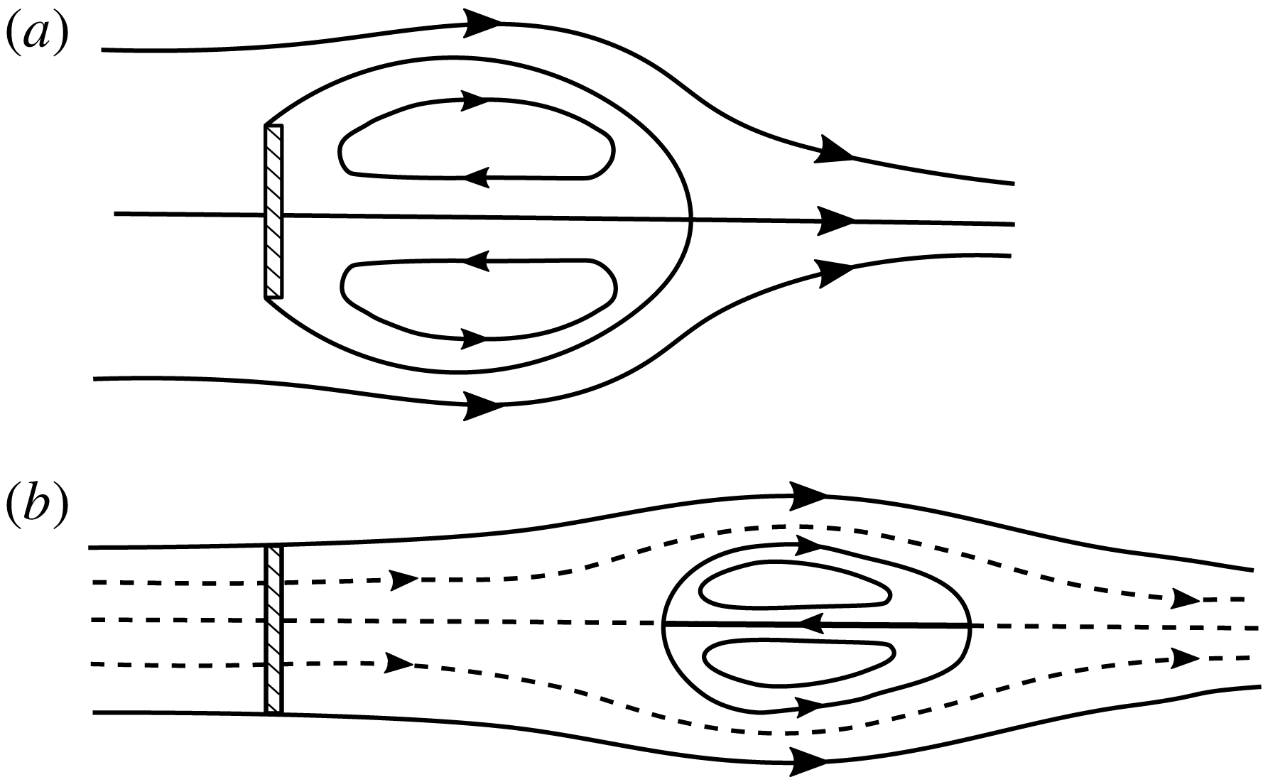
and showed that if the porosity is reduced below a critical value, the steady shear layers become unstable and the periodic Karman vortex street emerges. For porosities larger than the critical value, shedding is suppressed as the enhanced fluid bleeding inhibits the communication of the shear layers, similarly to a splitter plate. Furthermore, the ‘intensity’ of the shear layers has a strong effect on the recirculation region in the wake. For zero porosity (solid plate), this region is attached to the plate. As the porosity is increased, the recirculation region detaches from the plate, gradually moving downstream, as shown in figure 1.
The effect of porosity on the wake: (a)
 $\unicode[STIX]{x1D6FD}=0$
, (b)
 $\unicode[STIX]{x1D6FD}=0.3$
. Modified from Castro (Reference Castro1971).

The variety of possible regimes poses a significant challenge to the analytical prediction of the plate drag. Most existing models rely on potential flow theory, along with modified boundary conditions to ‘simulate’ important effects generated by viscosity. Betz (Reference Betz1920) considered potential flow everywhere apart from the region closest to the plate, and calculated the plate drag by applying a momentum budget in a control volume enclosing the plate. For large porosities, this model has been shown to work quite well, but the model becomes increasingly inaccurate as porosity is decreased. This is mainly because this model assumes that no mixing occurs between the outer flow and the wake, for the whole development of the wake region. While this assumption is acceptable when most of the fluid passes through the plate and the shear layers are ‘weak’, it generates inconsistencies if significant fluid volume circumvents the plate. In that case, intense mixing occurs, which causes a significant lowering of the wake pressure compared with the ambient, an effect termed ‘base suction’ (Roshko Reference Roshko1955). As this is not taken into account by the Betz model, its predictions underestimate the drag for small plate porosities, e.g. in the case of a solid plate, the model yields the unphysical prediction of zero drag.
The model of Betz (Reference Betz1920) produces the same prediction as the one of Taylor (Reference Taylor1944), in which the plate is represented by a distribution of sources of equal strength. Depending on the source strength, part of the free stream passes through the plate, while the rest circumvents the plate, diverted by a ‘Kutta-like’ boundary condition imposed by the sources. The resulting force is then readily calculated using Lagally’s theorem.
Koo & James (Reference Koo and James1973) proposed an improvement to the model, by including a more realistic description of the wake. The plate is again represented by a distribution of sources, but the resulting wake velocities are scaled down appropriately to fulfil the additional boundary condition of mass conservation across the plate. The drag is then calculated using Bernoulli’s equation before and after the plate. For large porosities, the predictions of this model have been shown to be close to those of Betz–Taylor, while there are improvements for lower porosities. For instance, for the solid plate limit (
 $\unicode[STIX]{x1D6FD}=0$
), the prediction of Koo & James (Reference Koo and James1973) is non-zero (compared with the zero prediction of Betz–Taylor), albeit much smaller than the experimentally observed value (see § 3). As will be shown below, the discrepancies between the model predictions and experimental observations are best explained by the neglected wake mixing and base suction.
As such, we may conclude that the models presented above are only valid for cases where the plate porosity is large. Otherwise, these models underestimate the drag, as they do not take into account the mixing of the outer flow with the wake region, and the subsequent base suction. A natural improvement would therefore be to allow the wake pressure to take values less than the ambient. This is the essence of the ‘notched’ hodograph methods of Roshko (Reference Roshko1954) and Cumberbatch (Reference Cumberbatch1981), for solid and porous plates respectively. However, apart from their complexity, the disadvantage of these models is that they require an a priori knowledge of the base pressure, e.g. from experimental measurements.
Here, we propose an analytical model (2.12) and (2.15) for the calculation of the drag of an infinite-aspect-ratio plate of arbitrary porosity, placed perpendicular to the free stream. This is achieved by extending the model of Koo & James (Reference Koo and James1973) by including a base-suction term. Drag and base suction are then solved simultaneously by applying momentum and energy conservation, rendering the model self-contained. The resulting predictions are compared with new experimental drag measurements and existing data from the literature, with convincing agreement.
2 Flow field model
2.1 A potential flow solution
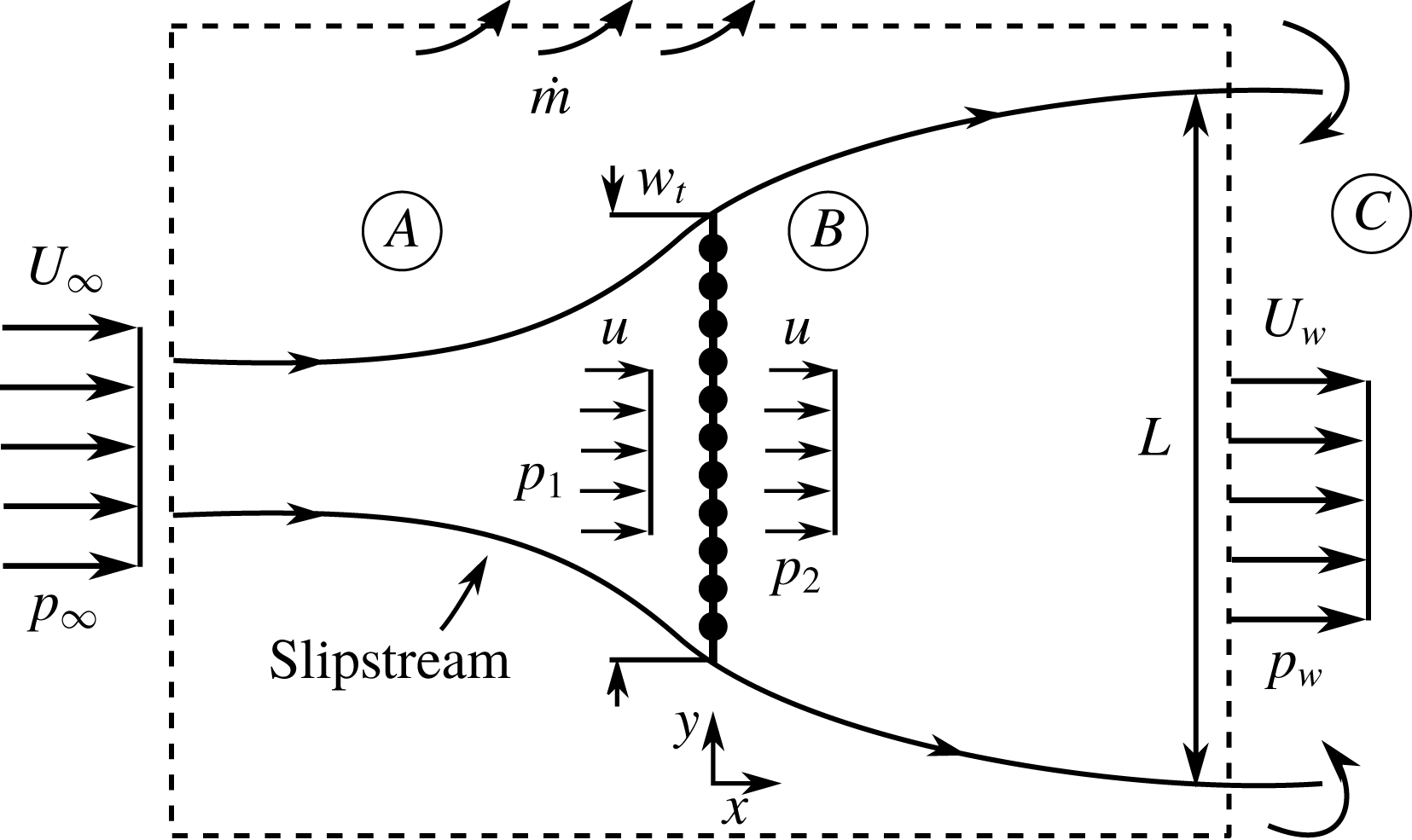
Following Taylor (Reference Taylor1944), we consider a distribution of potential sources of uniform strength
 $m$
along the
 $y$
axis representing the plate, combined with a free stream velocity
 $U_{\infty }$
parallel to the
 $x$
axis (see figure 2). The velocity upstream of the plate
 $u$
is the induced velocity at
 $x\rightarrow 0^{-}$
, namely
 $$\begin{eqnarray}\displaystyle u=U_{\infty }-\frac{m}{2}. & & \displaystyle\end{eqnarray}$$
The mass flux through the plate is then
 $\unicode[STIX]{x1D70C}uA$
, with
 $\unicode[STIX]{x1D70C}$
being the fluid density and
 $A$
the frontal gross area of the plate. If, like Taylor, we conclude the modelling at this step, the resulting force per unit area would be given using Lagally’s theorem as
 $\unicode[STIX]{x1D70C}mu$
, resulting in a drag coefficient of
 $C_{D}=4u/U_{\infty }(1-u/U_{\infty })$
, which could be interpreted as the combination of two effects: first, the diversion of the fluid around the plate and, second, the increase of the linear momentum of the fluid passing through the plate. Indeed, for
 $x\rightarrow 0^{+}$
, the induced streamwise velocity is given as
 $U_{\infty }+m/2>u$
. This increase in momentum is unrealistic, and in fact violates conservation of mass across the plate, but is necessary to keep the total pressure constant, as potential flow dictates. To account for these effects, and improve the predictions, the contribution of the momentum increase across the plate to the overall force needs to be accounted for, and the effects of base suction included. Then, the drag coefficient can be calculated using the formula
 $$\begin{eqnarray}\displaystyle C_{D}=\frac{p_{1}-p_{2}}{\frac{1}{2}\unicode[STIX]{x1D70C}U_{\infty }^{2}}, & & \displaystyle\end{eqnarray}$$
where
 $p_{1}$
and
 $p_{2}$
are the static pressures on the front and rear sides of the plate respectively.
2.2 A wake correction
Sketch of the flow field model, in which the plate is represented by a distribution of sources. The dashed lines bound the control volume where the momentum budget is applied.
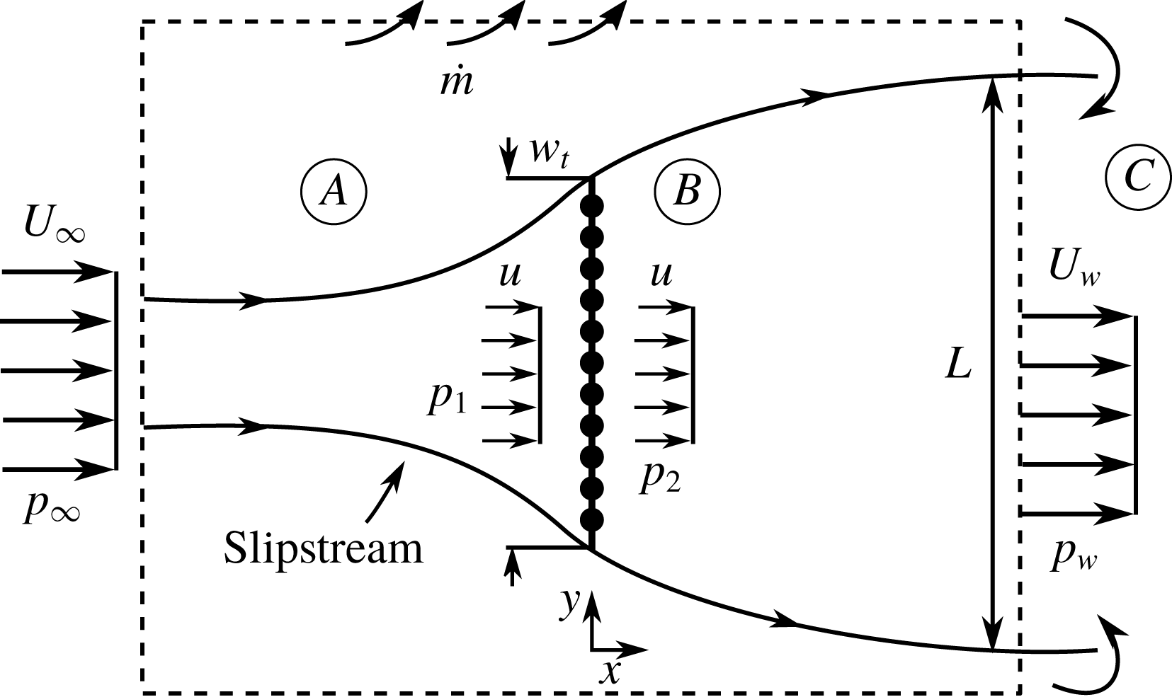
The flow can be divided into three regions, namely
 $A$
,
 $B$
and
 $C$
, as shown in figure 2. The flow in region
 $A$
(outside the wake bounded by the streamlines passing from the plate tips) is assumed to be inviscid and irrotational and its properties are determined using Taylor’s model as described above. Indeed, the measurements of Graham (Reference Graham1976) show that the mean streamwise velocity upstream of the plate is well represented by Taylor’s model for any porosity, including the solid plate case. Using Bernoulli’s equation, the following expression is obtained for
 $p_{1}$
:
 $$\begin{eqnarray}\displaystyle p_{1}=p_{\infty }+{\textstyle \frac{1}{2}}\unicode[STIX]{x1D70C}(U_{\infty }^{2}-u^{2}-v^{2}), & & \displaystyle\end{eqnarray}$$
where
 $v$
is the crosswise velocity immediately in front of the plate. This varies along the plate, but for simplicity is taken to be equal to its average value over the plate face, i.e. (see O’Neill Reference O’Neill2006)
 $$\begin{eqnarray}\displaystyle v^{2}=\frac{m^{2}}{12}=\frac{(U_{\infty }-u)^{2}}{3}. & & \displaystyle\end{eqnarray}$$
The flow in region
 $C$
is assumed to be viscous, and characterized by significant mixing with the outer flow. In region
 $C$
, the shear layers collapse, introducing a ‘base-suction’ effect, leading to a static pressure
 $p_{w}<p_{\infty }$
.
Following Koo & James (Reference Koo and James1973), we assume the flow in region
 $B$
to be inviscid, and the fluid to follow the streamlines predicted by Taylor’s model, but with its velocity scaled down appropriately such that mass is conserved across the plate. In that way, the artificial increase in mass, and consequently also momentum, of the flow passing through the plate predicted by Taylor’s model is negated. To do so, the wake velocities are multiplied with a factor
 $0\leqslant E\leqslant 1$
given by (note that (2.1) is used)
 $$\begin{eqnarray}\displaystyle E=\frac{U_{\infty }-{\displaystyle \frac{m}{2}}}{U_{\infty }+{\displaystyle \frac{m}{2}}}=\frac{u/U_{\infty }}{2-u/U_{\infty }}, & & \displaystyle\end{eqnarray}$$
so that the streamwise velocities for
 $x\rightarrow 0^{-}$
and
 $x\rightarrow 0^{+}$
coincide. Furthermore, we assume that no mixing occurs between the fluid of the outer region
 $A$
and that of region
 $B$
. Therefore, the total pressure is constant along a streamline in region
 $B$
, and
 $p_{2}$
is given by
 $$\begin{eqnarray}\displaystyle p_{2}=p_{w}+{\textstyle \frac{1}{2}}\unicode[STIX]{x1D70C}(U_{w}^{2}-u^{2}-v_{w}^{2}), & & \displaystyle\end{eqnarray}$$
where
 $v_{w}$
is the crosswise velocity immediately downstream of the plate, given by
 $v_{w}=Ev$
.
Next, we assume that the interface between regions
 $B$
and
 $C$
(i.e. the distance after which the shear layers collapse and mixing of the wake with the outer flow becomes significant) is far enough from the plate such that the flow velocity there is not influenced by the induced velocity from the source distribution, i.e.
 $U_{w}=U_{\infty }E$
.
Finally, combining (2.2)–(2.4) and (2.6), we obtain
 $$\begin{eqnarray}\displaystyle C_{D}=[1-E^{2}]\left[1-\frac{1}{3}\left(1-\frac{u}{U_{\infty }}\right)^{2}\right]-Cp_{w}, & & \displaystyle\end{eqnarray}$$
where
 $Cp_{w}=(p_{w}-p_{\infty })/((1/2)\unicode[STIX]{x1D70C}U_{\infty }^{2})$
. Equation (2.7) shows that the drag coefficient of a porous plate is the combination of two separate effects. First, the non-dimensional total pressure drop due to the fluid circumventing the plate, if base suction were absent, i.e.
 $[1-E^{2}]$
. This term is adjusted appropriately so that its contribution to the overall drag takes into account the static pressure decrease due to the crosswise velocity in the vicinity of the plate. As such, the term
 $[1-E^{2}]$
can be considered to quantify the ‘bluffness’ of the plate. Second, the term
 $-Cp_{w}$
, which represents the further decrease of the total pressure due to base suction.
It should be noted that (2.7) reduces to the prediction of Koo & James (Reference Koo and James1973) if we assume that
 $p_{w}=p_{\infty }$
(i.e. we neglect the added drag due to base suction) and neglect the effect of the crosswise velocity. Neglect of these terms represents the case of large plate porosity, which is where the prediction of Koo and James agrees well with experimental results.
2.3 Conservation of momentum
In the previous section, the drag coefficient was calculated based on energy conservation considerations. The computed drag, however, has to be consistent with conservation of momentum in a volume around the plate. This poses a constraint on the problem which can be used to calculate the base pressure term. It should be noted that a similar approach was used by Yeung & Parkinson (Reference Yeung and Parkinson2000) for solid plates and wedges.
Consider the control surface shown with a dashed line in figure 2. A momentum balance of the fluid passing through this surface requires
 $$\begin{eqnarray}\displaystyle D+(p_{w}-p_{\infty })L=\unicode[STIX]{x1D70C}L(U_{\infty }^{2}-U_{w}^{2})-{\dot{m}}U_{\infty }, & & \displaystyle\end{eqnarray}$$
where
 $D$
is the plate drag per unit length,
 $L$
is the wake width at the position where the control surface cuts the wake and
 ${\dot{m}}$
is the mass flow rate per unit length exiting the lateral control surfaces. Keeping in mind that
 $U_{w}=EU_{\infty }$
, the wake width can be calculated by applying conservation of mass inside the wake, i.e.
 $$\begin{eqnarray}\displaystyle L=\frac{u}{EU_{\infty }}w_{t}=\left(2-\frac{u}{U_{\infty }}\right)w_{t}, & & \displaystyle\end{eqnarray}$$
where
 $w_{t}$
is the plate width. It should be noted that for the solid plate case,
 $u=U_{w}=0$
, and thus the wake width cannot be calculated using conservation of mass. In that case, we use the limiting value of the wake width as the plate tends to become solid, i.e. using (2.9),
 $\lim _{u\rightarrow 0}L=2w_{t}$
.
The mass flow rate per unit length
 ${\dot{m}}$
can be calculated by applying conservation of mass outside the wake, i.e.
 $$\begin{eqnarray}\displaystyle {\dot{m}}=\unicode[STIX]{x1D70C}(U_{\infty }-EU_{\infty })L, & & \displaystyle\end{eqnarray}$$
where we have assumed that no mixing occurs between the outer flow and the wake. By combining (2.8), (2.9) and (2.10) and normalizing appropriately we obtain
 $$\begin{eqnarray}\displaystyle C_{D}=2E(1-E)\left(2-\frac{u}{U_{\infty }}\right)-Cp_{w}\left(2-\frac{u}{U_{\infty }}\right). & & \displaystyle\end{eqnarray}$$
Equation (2.11) shows that the drag of the plate is given as the difference of the momentum flux of the fluid entering and exiting the slipstream (first term on the right-hand side) plus the pressure forces on the control surface (second term on the right-hand side). In the special case of a solid plate (
 $u=E=0$
), (2.11) predicts a vanishing drag coefficient if, like Koo & James (Reference Koo and James1973), we assume that
 $Cp_{w}=0$
. However, their prediction for the same case is non-zero, showing that their model is inconsistent with conservation of momentum.
Making the substitution
 $u^{\ast }=u/U_{\infty }$
and using the definition of
 $E$
, i.e. (2.5), we finally obtain
 $$\begin{eqnarray}\displaystyle -Cp_{w} & = & \displaystyle \frac{8}{3}\left(\frac{1-u^{\ast }}{2-u^{\ast }}\right)^{2},\end{eqnarray}$$
 $$\begin{eqnarray}\displaystyle C_{D} & = & \displaystyle \frac{4}{3}\frac{(1-u^{\ast })(2+u^{\ast })}{(2-u^{\ast })}.\end{eqnarray}$$
2.4 Plate resistance
In the previous section, we calculated the drag connected with the fluid circumventing the plate, diverted by a ‘Kutta-like’ condition imposed by the sources, as a function of the velocity ratio
 $u/U_{\infty }$
. The latter, however, is not always easily known for a given plate geometry, limiting the practicality of the model. A more straightforward approach would be to use the easily measured plate open area ratio
 $\unicode[STIX]{x1D6FD}=A_{p}/A$
as the independent variable of the model instead. To do so, an additional equation is necessary, linking the drag coefficient and the open area ratio to
 $u/U_{\infty }$
. This relationship can be obtained by calculating the total pressure loss on a streamline that passes through the plate. The total pressure loss can be considered as a sum of viscous losses due to the friction between the plate walls and the fluid particles, and dynamic losses due to separation of the flow at the end of the contraction.
We consider a sufficiently large Reynolds number based on the pore dimensions, so that viscous forces can be neglected. It should be noted that for screens and fabrics constructed from cylindrical elements, Hoerner (Reference Hoerner1952) found a critical Reynolds number of
 $Re_{c}\approx 1000$
, based on the diameter of the cylindrical elements and the maximum velocity through the fabric, above which friction losses are negligible. Then, using Bernoulli’s equation, we may calculate the pressure of the fluid passing through the holes as
 $$\begin{eqnarray}\displaystyle p_{h}=p_{1}+{\textstyle \frac{1}{2}}\unicode[STIX]{x1D70C}u^{2}(1-1/\unicode[STIX]{x1D6FD}^{2})+{\textstyle \frac{1}{2}}\unicode[STIX]{x1D70C}v^{2}, & & \displaystyle\end{eqnarray}$$
where
 $v^{2}$
is given by (2.4). Immediately downstream of the holes, the flow separates, as it is discharged into the space behind the plate. As mentioned above, this results in total pressure losses, and when the fluid regains its initial velocity
 $u$
, its pressure will be
 $p_{2}<p_{1}$
. To model
 $p_{2}$
, we follow Taylor & Davies (Reference Taylor and Davies1944) and consider that all surplus kinetic energy due to the fluid acceleration is lost, and is thus not reconverted into pressure. Then, the total pressure after the flow has settled will be
 $$\begin{eqnarray}\displaystyle p_{2}+{\textstyle \frac{1}{2}}\unicode[STIX]{x1D70C}u^{2}+{\textstyle \frac{1}{2}}\unicode[STIX]{x1D70C}v_{w}^{2}=p_{h}+{\textstyle \frac{1}{2}}\unicode[STIX]{x1D70C}u^{2}, & & \displaystyle\end{eqnarray}$$
where
 $v_{w}$
is the crosswise velocity immediately downstream of the plate. By combining (2.13) and (2.14) and normalizing appropriately we obtain
 $$\begin{eqnarray}\displaystyle C_{D}=u^{\ast 2}\left(\frac{1}{\unicode[STIX]{x1D6FD}^{2}}-1\right)-\frac{4}{3}\frac{(1-u^{\ast })^{3}}{(2-u^{\ast })^{2}}. & & \displaystyle\end{eqnarray}$$
It should be noted that Taylor & Davies (Reference Taylor and Davies1944) considered a plate spanning the whole test section, and therefore neglected the crosswise velocities before and after the plate. In that case, (2.15) becomes
 $k=1/\unicode[STIX]{x1D6FD}^{2}-1$
, where
 $k=C_{D}U_{\infty }^{2}/u^{2}$
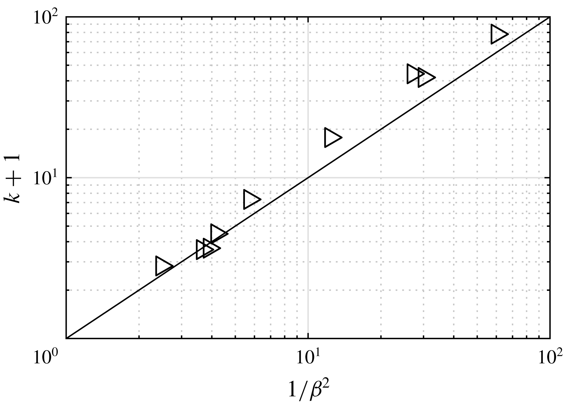
. Figure 3 shows that this relationship agrees quite well with experimental results taken from Taylor & Davies (Reference Taylor and Davies1944).
Variation of the resistance coefficient,
 $k=C_{D}U_{\infty }^{2}/u^{2}$
, of a porous sheet perpendicular to the free stream with the open area ratio. Symbols: measurements of porous plates spanning the whole test section from Taylor & Davies (Reference Taylor and Davies1944). Solid line:
 $k=(1-\unicode[STIX]{x1D6FD}^{2})/\unicode[STIX]{x1D6FD}^{2}$
.

To express the drag coefficient as a function of the plate open area ratio
 $\unicode[STIX]{x1D6FD}$
, we need to equate the two predictions for the drag coefficient, i.e. (2.12b
) and (2.15). Physically, this implies that the resistance a fluid particle faces to pass through the plate, in steady conditions, is equal to the resistance it would face were it to circumvent the plate. In the limit of zero porosity (
 $u=\unicode[STIX]{x1D6FD}=0$
), all fluid circumvents the plate and (2.12b
) is sufficient for the drag prediction (
 $C_{D}=4/3$
).
3 Validation and discussion
3.1 Experimental apparatus
Experiments were conducted in a water channel with a test section 0.46 m wide, 0.27 m deep and 2.44 m long. The mean free stream velocity was set to
 $0.2~\text{ms}^{-1}$
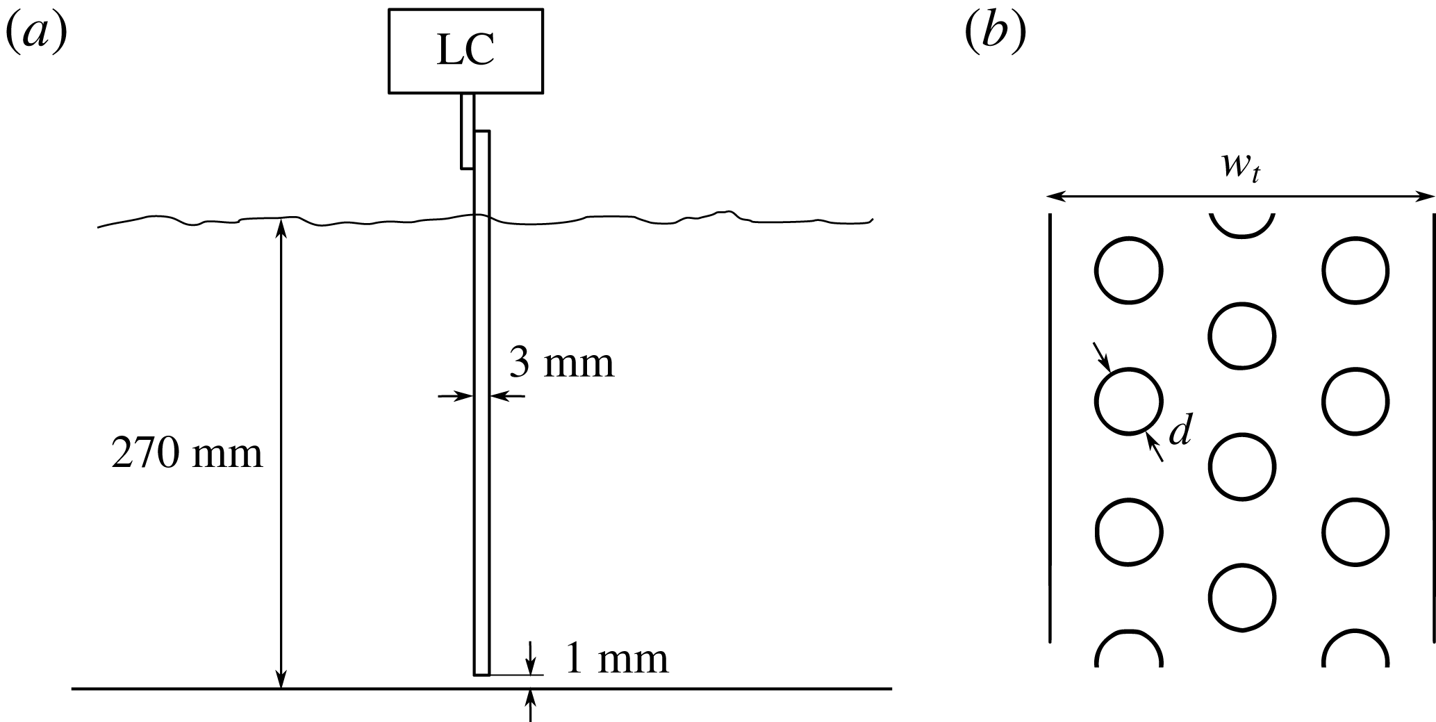
. A set of six perforated plates was tested, details of which can be seen in figure 4 and table 1. All plates were made from stainless steel with a thickness of 3 mm and with the same net area, leading to the same channel blockage ratio of 6.5 %. By varying the hole diameter and the gross plate area, a range of open area ratios
 $\unicode[STIX]{x1D6FD}=0{-}60\,\%$
was obtained. The plates were oriented perpendicular to the free stream, as shown in figure 4. This was done by rotating the plates using a stepper motor, and locating the angle where the plate drag was maximum. Care was taken so that the plates did not touch the channel bottom, but were separated by a small gap of approximately 1 mm. The Reynolds number based on the ‘net width’,
 $(1-\unicode[STIX]{x1D6FD})w_{t}$
, was
 $Re=6000$
for all plates tested, larger than the critical
 $Re_{c}=1000$
where the drag coefficient of solid square plates reaches a plateau (see Hoerner Reference Hoerner1965). Drag was measured using a load cell (ATI Mini40) with a force resolution of
 $5\times 10^{-3}$
N. Following previous studies involving perforated and solid plates (e.g. de Bray Reference de Bray1957; Castro Reference Castro1971; Bearman & Trueman Reference Bearman and Trueman1972), drag was corrected for blockage using the method of Maskell (Reference Maskell1965). To gain an idea about the experimental error, measurements were repeated for the plate
 $\unicode[STIX]{x1D6FD}=0.3$
four more times, on different days and experimental runs. An error bar was added (see figure 5) at that particular data point, representing the standard deviation of the five mean values.
(a) Side view of the water channel, the load cell (LC) and the plate. (b) Front view of a porous plate;
 $w_{t}$
and
 $d$
are given in table 1.

Geometrical characteristics of the tested plates.

For the three plates whose open area ratio was less than the critical value
 $\unicode[STIX]{x1D6FD}=0.23$
, where Castro (Reference Castro1971) observed that shedding emerged, measurements were also taken with a 1.5 mm thick stainless steel splitter plate positioned at the wake of the plates, spanning the whole channel height. The splitter plate was separated from the perforated plates by a gap of 5 mm, i.e. 0.17 times the solid plate width, and had a length of 210 mm, i.e. 7 times the solid plate width. As shown by Apelt & West (Reference Apelt and West1975), this length is sufficient to completely suppress the shedding in plates. The small gap is not expected to have any effect on the drag, since a splitter plate can be detached from the body and still suppress the shedding, as long as it is covers the position where the Karman street is formed. For a circular cylinder, Roshko (Reference Roshko1955) showed that this distance is 2.7 times the cylinder diameter, much larger than the current gap. To verify the above, measurements were repeated for the solid plate case after the gap was doubled. No noticeable difference in drag was observed.
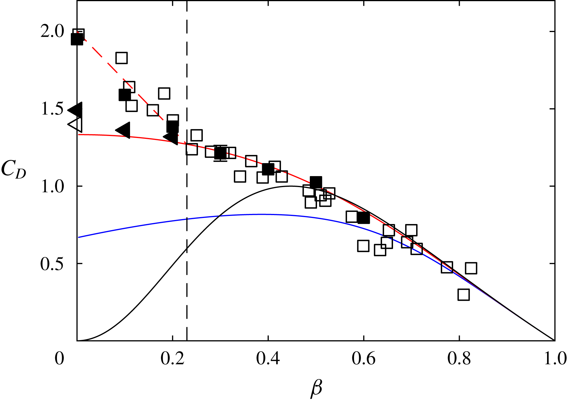
Plate drag coefficients against their open area ratios. Filled symbols: current measurements. Empty symbols: previous measurements taken from Graham (Reference Graham1976) and Bearman & Trueman (Reference Bearman and Trueman1972). Squares: no splitter plate. Triangles: splitter plate. Red line: current prediction (2.12b ) and (2.15). Black line: Prediction of the model of Betz–Taylor. Blue line: prediction of the model of Koo & James (Reference Koo and James1973). Dashed black line: point where shedding emerges, as measured by Castro (Reference Castro1971). Dashed red line: empirical fit capturing shedding.

3.2 Comparison with plate data
In figure 5, the drag coefficients of plates of varying porosity are plotted against their open area ratios. The data include the current measurements and data taken from the literature, i.e. from Bearman & Trueman (Reference Bearman and Trueman1972) for the solid case and from Graham (Reference Graham1976) for porous plates. Graham (Reference Graham1976) included results from his own experiments as well as data taken from previous studies.
In figure 5, the predictions of Betz–Taylor, Koo and James, and the current study, i.e. (2.12b
) and (2.15), are also plotted. We observe that both the predictions of Betz–Taylor and those of Koo and James can be considered to be valid only for
 $\unicode[STIX]{x1D6FD}>0.5$
. For smaller porosities, the Betz–Taylor model gives unphysical predictions, with the drag coefficient decreasing instead of increasing. The model of Koo & James (Reference Koo and James1973) also fails for large porosities, as it neglects the effect of base suction. It should be noted that in the study of Koo & James (Reference Koo and James1973), the graphical representation of their prediction does not exhibit the small drop when
 $\unicode[STIX]{x1D6FD}$
is small, but rather increases slowly until
 $C_{D}=1$
for
 $\unicode[STIX]{x1D6FD}=0$
. However, this increase is artificial and is because the crosswise velocity upstream of the plate,
 $v$
, is assumed to be negligible, resulting in the prediction
 $C_{D}=1-E^{2}$
(see discussion in § 2). While this assumption is reasonable for large
 $\unicode[STIX]{x1D6FD}$
, it is not true for small plate porosities, since in those cases the majority of the fluid volume has to circumvent the plate. A better representation of their model would be
 $C_{D}=[1-E^{2}][1-(1-u/U_{\infty })^{2}/3]$
(i.e. (2.7) without the base-suction term), which is represented by the blue line in figure 5.
The model proposed herein is shown as the solid red line in figure 5, and it agrees very well with the data for all porosities where shedding remains suppressed, i.e.
 $\unicode[STIX]{x1D6FD}\geqslant 0.23$
. For lower porosities, the data diverge from the prediction and can only be captured using an empirical fit. This is expected, as one of the model assumptions is that there is no mixing between region
 $B$
and the outer flow (see figure 2). This assumption is approximately true when shedding is absent, but invalid when shedding is present as it causes intense mixing in the wake. As such, when shedding is suppressed by the use of a splitter plate, the data fall close to the prediction for all porosities. In that case, the standard error of the model was found to be
 $S=0.08$
, defined as
 $$\begin{eqnarray}\displaystyle S=\sqrt{\frac{1}{n}\mathop{\sum }_{i=1}^{i=n}(y_{i}-f_{i})^{2}}, & & \displaystyle\end{eqnarray}$$
where
 $n$
is the number of data points,
 $y_{i}$
is the measurement at a particular open area ratio and
 $f_{i}$
is the prediction of (2.12b
) and (2.15) at the same open area ratio.
In the solid case, (2.12b
) predicts
 $C_{D}=1.33$
, while the experiments indicate
 $C_{D}=1.44\pm 0.4$
. This agreement is also reflected in the base pressure: (2.12b
) predicts
 $-Cp_{w}=0.67$
, which can be compared with the experimentally observed value of
 $-Cp_{w}=0.6$
for solid plates equipped with a splitter plate, as measured by Bearman & Trueman (Reference Bearman and Trueman1972).
4 Summary
A model for predicting the drag on a plate of arbitrary porosity is introduced. The model is formulated using potential flow theory, along with the following four conditions to render the flow field realistic. First, following Taylor (Reference Taylor1944), we impose a ‘Kutta-like’ boundary condition on the fluid that circumvents the plate. Second, following Taylor & Davies (Reference Taylor and Davies1944), we impose a total pressure loss on the fluid that passes through the plate. Third, following Koo & James (Reference Koo and James1973), we rescale the wake velocities to impose mass conservation on the fluid passing through the plate. Fourth, following Roshko (Reference Roshko1954), we allow the pressure in the far wake to take values less than the ambient. Drag is then calculated under the constraints of energy, momentum and mass conservation. The proposed model (2.12b ) and (2.15) captures better the flow physics associated with flow bleeding, and offers improved predictions compared with the classical Betz model, especially for small plate porosities. It could therefore find application in wind-turbine load and power predictions, through BEM, which relies heavily on drag predictions for porous plates.
Acknowledgements
We are grateful to Melissa Fan, for her help with the measurements. This research was funded by the National Science Foundation grant CBET-1652583 (Program Manager R. Joslin).