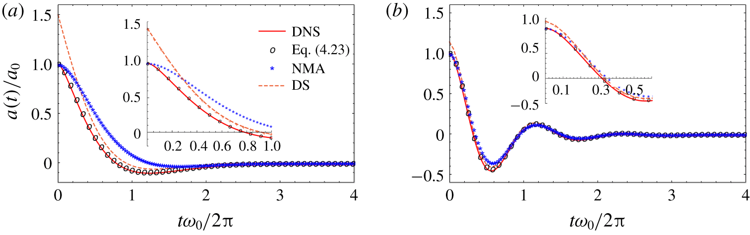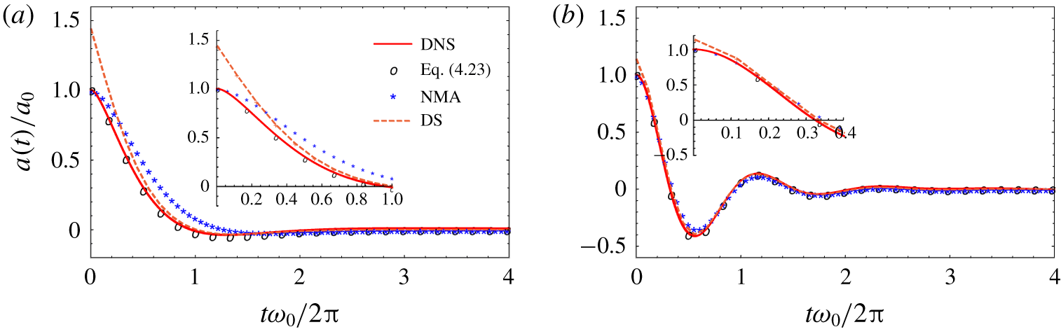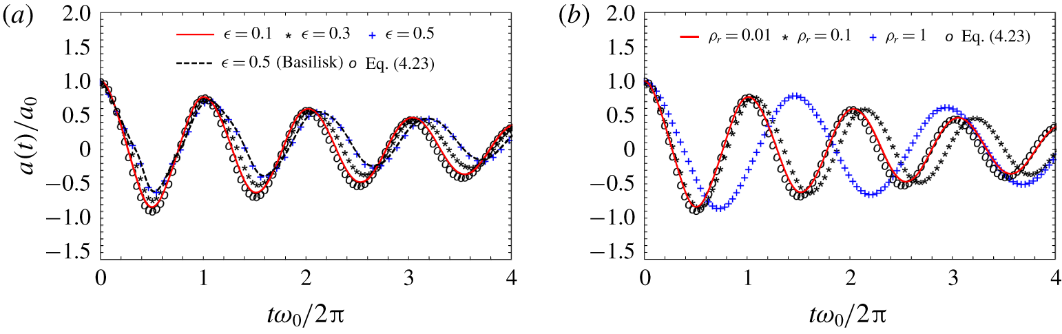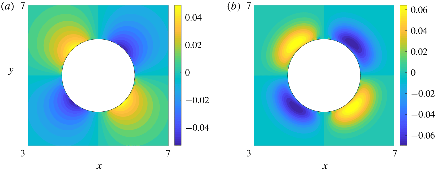


1 Introduction
Surface oscillations, instability, deformation and breakup of cylindrical gaseous filaments (density  $\unicode[STIX]{x1D70C}^{{\mathcal{I}}}$) surrounded by an immiscible fluid (density
 $\unicode[STIX]{x1D70C}^{{\mathcal{O}}}$) are of interest to numerous scientific applications e.g. microbubbles are obtained from breakup of a gaseous jet injected into a flowing liquid inside a T-junction (Garstecki et al. Reference Garstecki, Fuerstman, Stone and Whitesides2006) or a coaxial device (Castro-Hernández et al. Reference Castro-Hernández, van Hoeve, Lohse and Gordillo2011; Van Hoeve et al. Reference Van Hoeve, Dollet, Gordillo, Versluis, Van Wijngaarden and Lohse2011). The breakup of these cylindrical liquid or gaseous jets is often attributed to the Rayleigh–Plateau instability (Plateau Reference Plateau1873; Rayleigh Reference Rayleigh1892a; Van Hoeve et al. Reference Van Hoeve, Gekle, Snoeijer, Versluis, Brenner and Lohse2010) or to the pressure drop across the injected gas bubble (Garstecki et al. Reference Garstecki, Fuerstman, Stone and Whitesides2006; Castro-Hernández et al. Reference Castro-Hernández, van Hoeve, Lohse and Gordillo2011). In order to simplify analysis, stability studies of cylindrical jets or filaments (we use the word filament and jet interchangeably, the only difference being the absence or presence of an axial velocity profile, respectively, assumed here to be uniform (Chandrasekhar Reference Chandrasekhar1981; Eggers & Villermaux Reference Eggers and Villermaux2008)) are frequently conducted under one of two approximations for the density ratio. The first approximation
 $\unicode[STIX]{x1D70C}^{{\mathcal{O}}}/\unicode[STIX]{x1D70C}^{{\mathcal{I}}}\rightarrow 0$ describes a liquid jet issuing into an ambient gas (like air) of significantly lower density. The converse limit
 $\unicode[STIX]{x1D70C}^{{\mathcal{O}}}/\unicode[STIX]{x1D70C}^{{\mathcal{I}}}\rightarrow \infty$ corresponds to the so called ‘hollow jet’ approximation (Rayleigh Reference Rayleigh1892a; Chandrasekhar Reference Chandrasekhar1981; Eggers & Villermaux Reference Eggers and Villermaux2008) and applies to gaseous jets issuing into a (much) denser fluid, a recurrent situation in many microfluidic and chemical engineering applications.
The Rayleigh–Plateau instability (RP) is driven by surface tension and affects liquid as well as gaseous filaments. Inviscid, irrotational, linearised analysis (see Lin (Reference Lin2003) and Eggers & Villermaux (Reference Eggers and Villermaux2008) for exhaustive reviews) predicts that axisymmetric interfacial Fourier modes with wavelength greater than the circumference of the unperturbed filament are unstable and can lead to breakup. This may be seen from the dispersion relation (1.1) governing three-dimensional, irrotational perturbations on a cylindrical filament separating two inviscid, immiscible fluids (Rayleigh Reference Rayleigh1878, Reference Rayleigh1879, Reference Rayleigh1892a; Meister & Scheele Reference Meister and Scheele1967; Patankar, Farsoiya & Dasgupta Reference Patankar, Farsoiya and Dasgupta2018),
 $$\begin{eqnarray}\displaystyle \unicode[STIX]{x1D714}_{0}^{2}=\frac{T}{R_{0}^{3}}\left[\frac{kR_{0}\left(k^{2}R_{0}^{2}+m^{2}-1\right)}{\unicode[STIX]{x1D70C}^{{\mathcal{I}}}{\displaystyle \frac{\text{I}_{m}(kR_{0})}{\text{I}_{m}^{\prime }(kR_{0})}}-\unicode[STIX]{x1D70C}^{{\mathcal{O}}}{\displaystyle \frac{\text{K}_{m}(kR_{0})}{\text{K}_{m}^{\prime }(kR_{0})}}}\right]. & & \displaystyle\end{eqnarray}$$
Here  $\unicode[STIX]{x1D714}$ is the frequency,
 $k$ is the wavenumber of the interfacial, axial Fourier mode (
 $k\in \mathbb{R}^{+}$),
 $m$ is the index of the interfacial, azimuthal Fourier mode (
 $m\in \mathbb{Z}^{+}$),
 $R_{0}$ is the radius of the unperturbed filament,
 $T$ is surface tension and
 $\text{I}_{m}(\cdot )$ and
 $\text{K}_{m}(\cdot )$ are the
 $m$th-order, modified Bessel functions of the first and second kind, respectively. Note from (1.1) that while the RP instability criterion (
 $kR_{0}<1$) is the same for a liquid and a hollow filament, the most unstable wavelength (and its temporal growth rate) turns out to be higher for the hollow filament compared to a liquid filament of the same density (Rayleigh Reference Rayleigh1892a).
As is also seen from (1.1), the RP instability may be bypassed rather easily. As the denominator of (1.1) is always positive, imposing a three-dimensional ( $\propto \cos (m\unicode[STIX]{x1D703})\cos (kz),m>0,k\geqslant 0$), or even a purely azimuthal interfacial perturbation (
 $k=0,m\geqslant 2$) on the filament, produces simple harmonic oscillations at the interface. The case of purely azimuthal perturbations (
 $kR_{0}\rightarrow 0,m>0$) is particularly interesting. For such perturbations, the dispersion relation (1.1) reduces to (Rayleigh Reference Rayleigh1878; Bohr Reference Bohr1909; Fyfe, Oran & Fritts Reference Fyfe, Oran and Fritts1988)
 $$\begin{eqnarray}\displaystyle \unicode[STIX]{x1D714}_{0}^{2}=\frac{T}{R_{0}^{3}}\left[\frac{m(m^{2}-1)}{\unicode[STIX]{x1D70C}^{{\mathcal{I}}}+\unicode[STIX]{x1D70C}^{{\mathcal{O}}}}\right]. & & \displaystyle\end{eqnarray}$$
It is seen from (1.2) that azimuthal modes with  $m=2,3\ldots$ lead to oscillatory motion at the interface (in two dimensions
 $m=0$ and
 $1$ represent compressible and translational, zero frequency modes, respectively, and are not of interest). The study of such azimuthal capillary oscillations (the topic of the present study) have led to interesting applications. For example Rayleigh (Reference Rayleigh1889) proposed the use of (1.2) to estimate changes in dynamic surface tension of an elliptic liquid jet composed of water and oleate mixed in various proportions (see Pederson Reference Pederson1907). Niels Bohr (Bohr Reference Bohr1909) analytically determined the effect of viscosity (and individually that of weak nonlinearity or density of the ambient air) to (1.2). A number of experimental and theoretical investigations have subsequently examined the accuracy and limitations of the modifications to (1.2) proposed by Bohr (see Netzel, Hoch & Marx (Reference Netzel, Hoch and Marx1964), Ronay (Reference Ronay1978), Bechtel et al. (Reference Bechtel, Cooper, Forest, Petersson, Reichard, Saleh and Venkataramanan1995) and Moon et al. (Reference Moon, Shin, Kwak, Yang, Lee, Kim and An2016) and also page 72 of the review by Eggers & Villermaux (Reference Eggers and Villermaux2008)).
In many applications, inviscid-irrotational analysis may not be sufficient and it is necessary to incorporate viscous effects into (1.1) and (1.2). The dispersion relation governing small amplitude, axisymmetric perturbations on a viscous liquid cylinder was first obtained by Rayleigh (Reference Rayleigh1892b) (also see Tomotika (Reference Tomotika1935), Bauer (Reference Bauer1984), Stone & Brenner (Reference Stone and Brenner1996) and Liang et al. (Reference Liang, Deng, Nave and Johnson2011) for further results). For axisymmetric perturbations on a hollow filament surrounded by a viscous liquid, the corresponding dispersion relation is presented in Chandrasekhar (Reference Chandrasekhar1981) (also see Parthasarathy & Chiang (Reference Parthasarathy and Chiang1998)). Akin to inviscid results, in the viscous case as well, the wavelength of the most unstable axisymmetric mode (and its growth rate) is found to be higher for the hollow filament (Chandrasekhar Reference Chandrasekhar1981) when compared to a liquid filament of the same density and viscosity. An important feature of the temporal spectrum in these viscous problems on unbounded domains, is that it may not be purely discrete. For a given Fourier mode imposed on the interface, the viscous dispersion relation may admit a finite number of roots only, thus yielding a finite set of eigenfunctions. These eigenfunctions constituting the discrete spectrum, typically decay exponentially in space. Consequently any perturbation (e.g. in vorticity) imposed in the far field cannot be expressed as a linear combination of the discrete eigenmodes alone. In other words, the discrete spectrum eigenfunctions do not form a complete set and there is a continuum of eigenfunctions (labelled as the continuous spectrum), whose contribution may be large depending on fluid parameters and initial conditions. This is a common feature in viscous, interfacial perturbation problems occurring on unbounded domains e.g. capillary standing waves occurring on a rectangular (Cortelezzi & Prosperetti Reference Cortelezzi and Prosperetti1981; Prosperetti Reference Prosperetti1981; Prosperetti & Cortelezzi Reference Prosperetti and Cortelezzi1982; Lamb Reference Lamb1993) or cylindrical quiescent, viscous pool of liquid (Miles Reference Miles1968; Farsoiya, Mayya & Dasgupta Reference Farsoiya, Mayya and Dasgupta2017) of infinite depth, capillary standing waves on a bubble surrounded by radially unbounded viscous liquid (Prosperetti Reference Prosperetti1980a,Reference Prosperettib) etc. In addition to the set of problems mentioned above, the continuous spectrum has also been studied in the context of stability of thin film flows on a horizontally unbounded domain with bottom topography (Kalliadasis & Homsy Reference Kalliadasis and Homsy2001).
The possibility of the continuous spectrum for axisymmetric perturbations on a viscous liquid filament was first studied by Berger (Reference Berger1988) by solving the initial value problem with mixed initial conditions involving a surface deformation and an impulse (see § 2.2 in García & González (Reference García and González2008) for a survey of references on the inviscid, initial-value problem). The study by García & González (Reference García and González2008) has, however, negated some of the conclusions of Berger (Reference Berger1988) showing that the corresponding viscous dispersion relation admits infinite roots leading to a countably infinite set of eigenmodes. The results of García & González (Reference García and González2008) are consistent with similar conclusions drawn by Prosperetti (Reference Prosperetti1980b) earlier, for capillary perturbations on a liquid droplet. While the normal mode approach has been compared to the initial value problem (IVP) solution for a liquid filament (Berger Reference Berger1988; García & González Reference García and González2008), this has not been done for a hollow filament surrounded by a viscous fluid. In particular, for this problem the existence of the continuous spectrum in addition to the discrete spectrum has not been discussed in the literature before. In our present study we have assumed a quiescent base state, ignoring the possible presence of an axial velocity field. In this context, two relevant prior studies are by Parthasarathy & Chiang (Reference Parthasarathy and Chiang1998) and Gordillo, Gañán-Calvo & Pérez-Saborid (Reference Gordillo, Gañán-Calvo and Pérez-Saborid2001). Parthasarathy & Chiang (Reference Parthasarathy and Chiang1998) modelled a constant axial gas flow inside a cylindrical filament with zero velocity in the liquid outside (in the base state) obtaining the dispersion relation for three-dimensional perturbations using normal mode analysis. Imposition of an axial flow allows the possibility of the Kelvin–Helmholtz instability in addition to the Rayleigh–Plateau instability. The existence of the continuous spectrum was not mentioned by these authors. The study by Gordillo et al. (Reference Gordillo, Gañán-Calvo and Pérez-Saborid2001) has investigated the stability of a gas filament taking into account a base state axial velocity profile in the gas phase and the liquid phase, solving the perturbation equations using Laplace and Fourier transforms in time and space. These authors have, however, not discussed the continuous spectrum. Knowledge of the discrete spectrum and the continuous spectrum bears importance towards understanding and modelling of transient, free oscillations of a gaseous filament. As an example, consider a wave breaking in the ocean where a large (near) cylindrical column of air is entrained underneath a breaking wave (see figure 2 in Deike, Popinet & Melville (Reference Deike, Popinet and Melville2015)). In general, there may be azimuthal surface perturbations on these air columns and these are surrounded by a vortical velocity field in the fluid around, in the near and the far field. A first approximation to the effect of vorticity field on these perturbed air columns may be obtained from the study of the discrete and continuous spectrum eigenfunctions analysed here. Note that for these hollow air columns, gravity would produce a buoyant force which would cause the filament to accelerate upwards. This would in general alter the base state and we do not model these effects in the present study.
In hydrodynamic stability, a continuous spectrum arises due to the operator having singular points in the (possibly bounded) domain of interest or due to an unbounded domain (Friedman Reference Friedman1990). Formally a differential operator has a purely discrete spectrum if the associated integral operator happens to be compact. Continuous spectra that arise due to the former reason viz. the governing differential operator possesses singular points in the flow domain (Case Reference Case1960), play a fundamental role in non-modal growth of disturbances in shear flows (Roy & Subramanian Reference Roy and Subramanian2014a,Reference Roy and Subramanianb). In the current work the continuous spectrum occurs due to the latter reason, the presence of an infinite domain. The occurrence of a continuous spectrum in a viscous stability problem due to the unboundedness of the domain was first conjectured in the stability study of the Blasius boundary layer by Jordinson (Reference Jordinson1971). Mack (Reference Mack1976) supported this further using numerical calculations of the temporal stability problem which then received a formal mathematical characterization (Grosch & Salwen Reference Grosch and Salwen1978; Salwen & Grosch Reference Salwen and Grosch1981). The viscous continuous spectrum is crucial to the boundary layer’s receptivity as it can act as disturbance carrier for the free-stream turbulence, a feature that is lacking in the discrete modes. As discussed earlier, the viscous stability of interfacial flows also exhibits a continuous spectrum that renders the eigenfunction expansion complete (Miles Reference Miles1968; Prosperetti Reference Prosperetti1976, Reference Prosperetti1981; Farsoiya et al. Reference Farsoiya, Mayya and Dasgupta2017). In contrast to the planar problem where the continuous spectrum modes remain non-zero but bounded at infinity, continuous spectrum modes in the present study decay algebraically spatially. This is a manifestation of the cylindrical geometry and is reminiscent of the viscous continuous spectrum in the Batchelor vortex (Mao & Sherwin Reference Mao and Sherwin2011), a swirling flow with an axial jet modelling a trailing vortex. The continuous spectrum of the Batchelor vortex comprises of two families – potential and free-stream modes. The free-stream modes are analogous to the planar Blasius boundary layer modes, remaining finite at large distances, while the potential modes decay algebraically. A hollow filament does not have any imposed flow, hence ruling out the possibility of free-stream modes. The algebraically decaying ‘potential modes’ are thus the only candidates possible for the continuous spectrum of the hollow filament.
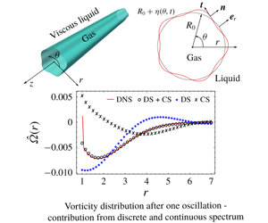
We analyse here the discrete and the continuous spectrum for purely azimuthal perturbations on a hollow cylindrical filament. Our analysis complements and extends earlier results on the continuous spectrum by Lamb (Reference Lamb1993), Prosperetti (Reference Prosperetti1976, Reference Prosperetti1981), Miles (Reference Miles1968), Farsoiya et al. (Reference Farsoiya, Mayya and Dasgupta2017) in other geometries to the present case of a hollow cylindrical filament. We demonstrate analytically the existence of the discrete and the continuous spectrum and show that an initial perturbation in the form of an interfacial Fourier mode and zero perturbation vorticity, has projections on the discrete as well as the continuous spectrum eigenfunctions. Consequently, it produces damped standing waves whose temporal evolution is not well approximated by a sum of exponentials (Prosperetti Reference Prosperetti1976, Reference Prosperetti1980a,Reference Prosperettib, Reference Prosperetti1981; Farsoiya et al. Reference Farsoiya, Mayya and Dasgupta2017), especially at early times. We validate our normal mode analysis by also solving the initial value problem. All analytical predictions are tested against direct numerical simulations (DNS) conducted using a code developed in-house. The study is organised as follows: the linearised equations and boundary conditions are presented in § 2. We perform normal mode analysis in § 3.1 obtaining the viscous dispersion relation governing the discrete spectrum. Using normal mode analysis we demonstrate in § 3.2, the existence of an additional, uncountably infinite set of radial eigenmodes constituting the continuous spectrum. The discrete and the continuous modes together lead to a completeness relation for perturbation vorticity in § 3.3. We validate the normal mode predictions by solving the linearised IVP in (4.1). The in-house code used for DNS is described in § 5. We compare our analytical predictions to DNS in § 6. The study concludes with a summary and scope of future work.
2 Governing equations and boundary conditions – hollow filament
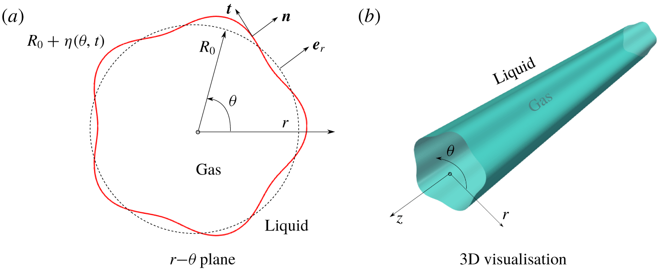
(a) A perturbed gas filament. (b) Three-dimensional visualisation of the filament.

As seen in figure 1(a,b), the base state consists of an infinitely long cylindrical gaseous filament of radius  $R_{0}$. The fluid outside the filament is taken to be radially unbounded and is quiescent in the base state with density and kinematic viscosity
 $\unicode[STIX]{x1D70C}$ and
 $\unicode[STIX]{x1D708}$, respectively. We ignore the dynamic effect of the gas inside the filament assuming it to be a low density, low viscosity, incompressible quiescent gas, exerting negligible stress at the interface (hollow filament approximation). The interface is thus free of tangential stresses at all times and we solve only for the fluid outside the filament. We take into account surface tension while neglecting gravity in subsequent analysis. Subject to these approximations, we solve for the flow generated in the fluid outside the filament due to linearised perturbations taken to be of standing wave form. The incompressible Navier–Stokes and continuity equations govern the total velocity
 $\boldsymbol{u}^{tot}$ and total pressure fields
 $p^{tot}$ viz.
 $$\begin{eqnarray}\displaystyle \frac{\text{D}\boldsymbol{u}^{tot}}{\text{D}t}=-\frac{1}{\unicode[STIX]{x1D70C}}\unicode[STIX]{x1D735}p^{tot}+\unicode[STIX]{x1D708}\unicode[STIX]{x1D6FB}^{2}\boldsymbol{u}^{tot},\quad \unicode[STIX]{x1D735}\boldsymbol{\cdot }\boldsymbol{u}^{tot}=0. & & \displaystyle\end{eqnarray}$$
All variables (with superscript  $tot$ standing for total) may be written as a sum of base and perturbation variables as,
 $$\begin{eqnarray}\displaystyle \boldsymbol{u}^{tot}=\mathbf{0}+\boldsymbol{u},\quad p^{tot}=-\frac{T}{R_{0}}+p, & & \displaystyle\end{eqnarray}$$
where  $T$ is the gas–liquid surface tension and
 $R_{0}$ is the unperturbed radius of the circular filament. As we do not solve for the gas inside the filament, the base state pressure inside the filament is taken to be zero (gas inside exerts negligible pressure) in our analysis implying that the base state pressure in the fluid outside the filament is negative. This is implied in the second of (2.2). Linearised equations governing the perturbations may be obtained using the standard procedure of substituting (2.2) into (2.1), subtracting the base state and retaining only up to linear order in perturbation variables. The resultant equations are the linearised, incompressible Navier–Stokes equations along with the continuity equation for perturbation velocity
 $\boldsymbol{u}$ and perturbation pressure
 $p$ viz.
 $$\begin{eqnarray}\displaystyle \frac{\unicode[STIX]{x2202}\boldsymbol{u}}{\unicode[STIX]{x2202}t}=-\frac{1}{\unicode[STIX]{x1D70C}}\unicode[STIX]{x1D735}p+\unicode[STIX]{x1D708}\unicode[STIX]{x1D6FB}^{2}\boldsymbol{u},\quad \unicode[STIX]{x1D735}\boldsymbol{\cdot }\boldsymbol{u}=0. & & \displaystyle\end{eqnarray}$$
As the perturbation treated here is pure azimuthal, our analysis is two-dimensional and we choose to solve equations (2.3) in the stream-function–vorticity formulation in cylindrical plane polar coordinates. The curl of the momentum equation in (2.3) leads to the equation for vorticity ( $\unicode[STIX]{x1D74E}\equiv \unicode[STIX]{x1D735}\times \boldsymbol{u}$). Expressing velocity in terms of a vector streamfunction
 $\unicode[STIX]{x1D74D}$ using
 $\boldsymbol{u}\equiv -\unicode[STIX]{x1D735}\times \unicode[STIX]{x1D74D}$ (the negative sign is for convenience) and using standard vector identities, leads to the following equations written in the (perturbation) stream-function–vorticity formulation (in two dimensions):
 $$\begin{eqnarray}\displaystyle \frac{\unicode[STIX]{x2202}\unicode[STIX]{x1D74E}}{\unicode[STIX]{x2202}t}=\unicode[STIX]{x1D708}\unicode[STIX]{x1D6FB}^{2}\unicode[STIX]{x1D74E},\quad \unicode[STIX]{x1D6FB}^{2}\unicode[STIX]{x1D74D}=\unicode[STIX]{x1D74E}. & & \displaystyle\end{eqnarray}$$
For two-dimensional flow the only non-zero component of vorticity and streamfunction is the out-of-plane  $z$ component i.e.
 $\unicode[STIX]{x1D74E}=(0,0,\unicode[STIX]{x1D714}(r,\unicode[STIX]{x1D703},t))$ and
 $\unicode[STIX]{x1D74D}=(0,0,\unicode[STIX]{x1D713}(r,\unicode[STIX]{x1D703},t))$ (see figure 1b). Projecting equations (2.4) into a cylindrical system (
 $r$-
 $\unicode[STIX]{x1D703}$-
 $z$), we obtain the
 $z$ component of these equations viz.
 $$\begin{eqnarray}\displaystyle & \displaystyle \frac{\unicode[STIX]{x2202}\unicode[STIX]{x1D714}}{\unicode[STIX]{x2202}t}=\unicode[STIX]{x1D708}\left(\frac{\unicode[STIX]{x2202}^{2}\unicode[STIX]{x1D714}}{\unicode[STIX]{x2202}r^{2}}+\frac{1}{r}\frac{\unicode[STIX]{x2202}\unicode[STIX]{x1D714}}{\unicode[STIX]{x2202}r}+\frac{1}{r^{2}}\frac{\unicode[STIX]{x2202}^{2}\unicode[STIX]{x1D714}}{\unicode[STIX]{x2202}\unicode[STIX]{x1D703}^{2}}\right), & \displaystyle\end{eqnarray}$$
 $$\begin{eqnarray}\displaystyle & \displaystyle \frac{\unicode[STIX]{x2202}^{2}\unicode[STIX]{x1D713}}{\unicode[STIX]{x2202}r^{2}}+\frac{1}{r}\frac{\unicode[STIX]{x2202}\unicode[STIX]{x1D713}}{\unicode[STIX]{x2202}r}+\frac{1}{r^{2}}\frac{\unicode[STIX]{x2202}^{2}\unicode[STIX]{x1D713}}{\unicode[STIX]{x2202}\unicode[STIX]{x1D703}^{2}}=\unicode[STIX]{x1D714}. & \displaystyle\end{eqnarray}$$
We may obtain the radial and azimuthal components of the two-dimensional perturbation velocity field  $\boldsymbol{u}=(u_{r},u_{\unicode[STIX]{x1D703}},0)$ from the perturbation streamfunction
 $\unicode[STIX]{x1D713}(r,\unicode[STIX]{x1D703},t)$ using
 $u_{r}=-(1/r)(\unicode[STIX]{x2202}\unicode[STIX]{x1D713}/\unicode[STIX]{x2202}\unicode[STIX]{x1D703}),u_{\unicode[STIX]{x1D703}}=(\unicode[STIX]{x2202}\unicode[STIX]{x1D713}/\unicode[STIX]{x2202}r)$. These relations follow from the definition
 $\boldsymbol{u}\equiv -\unicode[STIX]{x1D735}\times \unicode[STIX]{x1D74D}$ used earlier in obtaining (2.4).
In order to impose boundary conditions, we define a scalar field  $F$ and a unit normal and tangent,
 $\boldsymbol{n}$ and
 $\boldsymbol{t}$, respectively, (forming a right-handed coordinate system), to the perturbed interface,
 $$\begin{eqnarray}\displaystyle F(r,\unicode[STIX]{x1D703},t)\equiv r-R_{0}-\unicode[STIX]{x1D702}(\unicode[STIX]{x1D703},t),\quad \boldsymbol{n}\equiv \frac{\unicode[STIX]{x1D735}F}{|\unicode[STIX]{x1D735}F|}. & & \displaystyle\end{eqnarray}$$
As shown in figure 1(a),  $\unicode[STIX]{x1D702}(\unicode[STIX]{x1D703},t)$ represents the interfacial perturbation. The boundary conditions to be enforced are the kinematic boundary condition, zero shear stress and jump in normal stress due to surface tension, all at the interface. Additionally because our domain is radially unbounded, there are boundedness conditions for all variables, as
 $r\rightarrow \infty$. The mathematical expressions for these are, respectively, (Leal Reference Leal2007)
 $$\begin{eqnarray}\displaystyle & \displaystyle \left(\frac{\text{D}\unicode[STIX]{x1D702}}{\text{D}t}-\boldsymbol{u}^{tot}\boldsymbol{\cdot }\boldsymbol{e}_{r}\right)_{r=R_{0}+\unicode[STIX]{x1D702}}=0, & \displaystyle\end{eqnarray}$$
 $$\begin{eqnarray}\displaystyle & \displaystyle \left(\boldsymbol{t}\boldsymbol{\cdot }\unicode[STIX]{x1D748}^{tot}\boldsymbol{\cdot }\boldsymbol{n}\right)_{r=R_{0}+\unicode[STIX]{x1D702}}=0, & \displaystyle\end{eqnarray}$$
and
 $$\begin{eqnarray}\displaystyle \left(\boldsymbol{n}\boldsymbol{\cdot }\unicode[STIX]{x1D748}^{tot}\boldsymbol{\cdot }\boldsymbol{n}-T\unicode[STIX]{x1D735}\boldsymbol{\cdot }\boldsymbol{n}\right)_{r=R_{0}+\unicode[STIX]{x1D702}}=0, & & \displaystyle\end{eqnarray}$$
where the stress strain-rate relation,  $\unicode[STIX]{x1D748}^{tot}=-p^{tot}\unicode[STIX]{x1D644}+\unicode[STIX]{x1D707}[\unicode[STIX]{x1D735}\boldsymbol{u}^{tot}+(\unicode[STIX]{x1D735}\boldsymbol{u}^{tot})^{\text{T}}]$ applies to a Newtonian fluid. Note that
 $\boldsymbol{e}_{r}$ is a unit normal to the unperturbed interface, as shown in figure 1(a). Projecting equations (2.8)–(2.10) on a plane polar (
 $r,\unicode[STIX]{x1D703}$) coordinate system, using the decomposition (2.2) and expressing (perturbation) velocity components in terms of the (perturbation) stream function while retaining up to linear terms in perturbed quantities we obtain,
 $$\begin{eqnarray}\displaystyle & \displaystyle \frac{\unicode[STIX]{x2202}\unicode[STIX]{x1D702}}{\unicode[STIX]{x2202}t}+\left(\frac{1}{r}\frac{\unicode[STIX]{x2202}\unicode[STIX]{x1D713}}{\unicode[STIX]{x2202}\unicode[STIX]{x1D703}}\right)_{r=R_{0}}=0, & \displaystyle\end{eqnarray}$$
 $$\begin{eqnarray}\displaystyle & \displaystyle \unicode[STIX]{x1D707}\left(\frac{\unicode[STIX]{x2202}^{2}\unicode[STIX]{x1D713}}{\unicode[STIX]{x2202}r^{2}}-\frac{1}{r}\frac{\unicode[STIX]{x2202}\unicode[STIX]{x1D713}}{\unicode[STIX]{x2202}r}-\frac{1}{r^{2}}\frac{\unicode[STIX]{x2202}^{2}\unicode[STIX]{x1D713}}{\unicode[STIX]{x2202}\unicode[STIX]{x1D703}^{2}}\right)_{r=R_{0}}=0, & \displaystyle\end{eqnarray}$$
 $$\begin{eqnarray}\displaystyle & \displaystyle p(R_{0},\unicode[STIX]{x1D703},t)+2\unicode[STIX]{x1D707}\left(\frac{1}{r}\frac{\unicode[STIX]{x2202}^{2}\unicode[STIX]{x1D713}}{\unicode[STIX]{x2202}r\unicode[STIX]{x2202}\unicode[STIX]{x1D703}}-\frac{1}{r^{2}}\frac{\unicode[STIX]{x2202}\unicode[STIX]{x1D713}}{\unicode[STIX]{x2202}\unicode[STIX]{x1D703}}\right)_{r=R_{0}}=\frac{T}{R_{0}^{2}}\left(\unicode[STIX]{x1D702}+\frac{\unicode[STIX]{x2202}^{2}\unicode[STIX]{x1D702}}{\unicode[STIX]{x2202}\unicode[STIX]{x1D703}^{2}}\right), & \displaystyle\end{eqnarray}$$
and
 $$\begin{eqnarray}\displaystyle \lim _{r\rightarrow \infty }\unicode[STIX]{x1D714}(r,\unicode[STIX]{x1D703},t)\rightarrow \text{finite},\quad \lim _{r\rightarrow \infty }\unicode[STIX]{x1D713}(r,\unicode[STIX]{x1D703},t)\rightarrow \text{finite}. & & \displaystyle\end{eqnarray}$$
In further analysis, we use governing equations (2.5) and (2.6) along with boundary conditions (2.11)–(2.14).
3 Linear stability analysis – normal modes
Here we conduct a temporal stability analysis on the base state described earlier. An azimuthal Fourier mode of the form  $\cos (m\unicode[STIX]{x1D703})$ is imposed at the interface (see figure 1a) and we solve for the eigenvalues and the radial part of the eigenfunctions, using the normal mode approach. This implies setting the temporal dependency for all field variables to be of the form
 $\exp (\unicode[STIX]{x1D70E}t)$. It will emerge from this analysis that for a given value of
 $m$ and Laplace number,
 $La\equiv (TR_{0}\unicode[STIX]{x1D70C}/\unicode[STIX]{x1D707}^{2})$, the problem admits a discrete and a continuous spectrum. The discrete part of the spectrum is analysed in the following sub-section.
3.1 Normal modes – discrete spectrum
Due to variable separability, we seek normal mode solutions in the form of standing waves and set,
 $$\begin{eqnarray}\displaystyle & \displaystyle \unicode[STIX]{x1D702}(\unicode[STIX]{x1D703},t)=a_{0}\cos (m\unicode[STIX]{x1D703})\left[{\textstyle \frac{1}{2}}\exp (\unicode[STIX]{x1D70E}t)+\text{c.c.}\right], & \displaystyle\end{eqnarray}$$
 $$\begin{eqnarray}\displaystyle & \displaystyle \unicode[STIX]{x1D714}(r,\unicode[STIX]{x1D703},t)=\sin (m\unicode[STIX]{x1D703})\left[{\textstyle \frac{1}{2}}\unicode[STIX]{x1D6FA}(r)\exp (\unicode[STIX]{x1D70E}t)+\text{c.c.}\right], & \displaystyle\end{eqnarray}$$
 $$\begin{eqnarray}\displaystyle & \displaystyle \unicode[STIX]{x1D713}(r,\unicode[STIX]{x1D703},t)=\sin (m\unicode[STIX]{x1D703})\left[{\textstyle \frac{1}{2}}\unicode[STIX]{x1D6F9}(r)\exp (\unicode[STIX]{x1D70E}t)+\text{c.c.}\right], & \displaystyle\end{eqnarray}$$
 $$\begin{eqnarray}\displaystyle & \displaystyle p(r,\unicode[STIX]{x1D703},t)=\cos (m\unicode[STIX]{x1D703})\left[{\textstyle \frac{1}{2}}{\mathcal{P}}(r)\exp (\unicode[STIX]{x1D70E}t)+\text{c.c.}\right], & \displaystyle\end{eqnarray}$$
where  $\text{c.c.}$ stands for complex conjugate. Here
 $\unicode[STIX]{x1D6FA}(r),\unicode[STIX]{x1D6F9}(r)$ and
 ${\mathcal{P}}(r)$ are the eigenfunctions while
 $\unicode[STIX]{x1D70E}$ is related to the eigenvalue. We assume that
 $a_{0}$ and
 $m$ are real (the latter restricted to only integer values for periodicity,
 $m\in \mathbb{Z}^{+}$) while
 $\unicode[STIX]{x1D70E}$ is allowed to be complex (temporal analysis). Due to
 $\unicode[STIX]{x1D70E}$ being complex,
 $\unicode[STIX]{x1D6FA}(r),\unicode[STIX]{x1D6F9}(r)$ and
 ${\mathcal{P}}(r)$ are complex functions of a real argument as will be seen in the subsequent algebra. Substituting (3.2) and (3.3) into equations (2.5) and (2.6), we obtain
 $$\begin{eqnarray}\displaystyle \left[\frac{\text{d}^{2}\unicode[STIX]{x1D6FA}}{\text{d}r^{2}}+\frac{1}{r}\frac{\text{d}\unicode[STIX]{x1D6FA}}{\text{d}r}-\left(\frac{m^{2}}{r^{2}}+\frac{\unicode[STIX]{x1D70E}}{\unicode[STIX]{x1D708}}\right)\unicode[STIX]{x1D6FA}\right]\frac{\exp (\unicode[STIX]{x1D70E}t)}{2}+\text{c.c.}=0, & & \displaystyle\end{eqnarray}$$
and
 $$\begin{eqnarray}\displaystyle \left[\frac{\text{d}^{2}\unicode[STIX]{x1D6F9}}{\text{d}r^{2}}+\frac{1}{r}\frac{\text{d}\unicode[STIX]{x1D6F9}}{\text{d}r}-\frac{m^{2}}{r^{2}}\unicode[STIX]{x1D6F9}-\unicode[STIX]{x1D6FA}\right]\frac{\exp (\unicode[STIX]{x1D70E}t)}{2}+\text{c.c.}=0. & & \displaystyle\end{eqnarray}$$
For (3.5) and (3.6) to hold at all time  $t$, the coefficient of
 $\exp (\unicode[STIX]{x1D70E}t)/2$ (or equivalently that of
 $\exp (\bar{\unicode[STIX]{x1D70E}}t)/2$), must be zero. The resultant equations are,
 $$\begin{eqnarray}\displaystyle & \displaystyle \frac{\text{d}^{2}\unicode[STIX]{x1D6FA}}{\text{d}r^{2}}+\frac{1}{r}\frac{\text{d}\unicode[STIX]{x1D6FA}}{\text{d}r}-\left(\frac{\unicode[STIX]{x1D70E}}{\unicode[STIX]{x1D708}}+\frac{m^{2}}{r^{2}}\right)\unicode[STIX]{x1D6FA}=0, & \displaystyle\end{eqnarray}$$
 $$\begin{eqnarray}\displaystyle & \displaystyle \frac{\text{d}^{2}\unicode[STIX]{x1D6F9}}{\text{d}r^{2}}+\frac{1}{r}\frac{\text{d}\unicode[STIX]{x1D6F9}}{\text{d}r}-\frac{m^{2}}{r^{2}}\unicode[STIX]{x1D6F9}=\unicode[STIX]{x1D6FA}. & \displaystyle\end{eqnarray}$$
Note that equation (3.7) has complex coefficients (since  $\unicode[STIX]{x1D70E}\in \mathbb{C}$). Consequently both
 $\unicode[STIX]{x1D6FA}(r)$ and
 $\unicode[STIX]{x1D6F9}(r)$ are complex functions of
 $r$ (equation (3.8) has real coefficients but a complex inhomogenous term). The solution to equation (3.7) is
 $$\begin{eqnarray}\displaystyle \unicode[STIX]{x1D6FA}(r)={\mathcal{C}}\text{K}_{m}(lr)+{\mathcal{D}}\text{I}_{m}(lr), & & \displaystyle\end{eqnarray}$$
where  ${\mathcal{C}},{\mathcal{D}}$ are (complex) constants of integration and
 $\text{I}_{m},\text{K}_{m}$ are
 $m$th-order, modified Bessel functions of the first and second kind, respectively. We define
 $l\equiv \sqrt{\unicode[STIX]{x1D70E}/\unicode[STIX]{x1D708}}$, noting that
 $l$ is like a wavenumber having the dimensions of inverse length. In the subsequent algebra we write our equations in terms of
 $l$, replacing all instances of
 $\unicode[STIX]{x1D70E}$ with
 $\unicode[STIX]{x1D708}l^{2}$.
In order to prevent divergence of  $\unicode[STIX]{x1D6FA}(r)$ as
 $r\rightarrow \infty$, we set
 ${\mathcal{D}}=0$ in (3.9). We are thus implicitly assuming that
 $\text{Re}(l)>0$ (
 $\text{Re}(z)$ and
 $\text{Im}(z)$ denote the real and imaginary part of
 $z$), since for fixed
 $m$ and
 $z\rightarrow \infty$,
 $\text{I}_{m}(z)$ is asymptotic to
 $\exp (z)/\sqrt{2\unicode[STIX]{x03C0}z}$ (Abramowitz & Stegun Reference Abramowitz and Stegun1965) which diverges as
 $z\rightarrow \infty$ only if
 $\text{Re}(z)>0$. With
 $\unicode[STIX]{x1D6FA}(r)={\mathcal{C}}\text{K}_{m}(lr)$ from (3.9), the solution to (3.8) can be written as a linear combination of the two independent homogenous solutions
 $v_{1}(r)=r^{m}$ and
 $v_{2}(r)=r^{-m}$ and the particular integral (see equation (2.2.13) in Prosperetti (Reference Prosperetti2011) and the algebra in the supplementary material available at https://doi.org/10.1017/jfm.2019.809). This is,
 $$\begin{eqnarray}\displaystyle \unicode[STIX]{x1D6F9}(r)=\left[\unicode[STIX]{x1D6FC}+{\mathcal{C}}\int _{\infty }^{r}\frac{q^{-m+1}\text{K}_{m}\left(\hat{q}\right)}{2m}\,\text{d}q\right]r^{m}+\left[\unicode[STIX]{x1D6FD}-{\mathcal{C}}\int _{R_{0}}^{r}\frac{q^{m+1}\text{K}_{m}\left(\hat{q}\right)}{2m}\,\text{d}q\right]r^{-m}. & & \displaystyle\end{eqnarray}$$
Here  $\unicode[STIX]{x1D6FC}$ and
 $\unicode[STIX]{x1D6FD}$ are real constants of integration (since coefficients of the left-hand side of (3.8) are real) whose value depends on the choice of the lower limits of integration and
 $\hat{q}\equiv q\sqrt{\unicode[STIX]{x1D70E}/\unicode[STIX]{x1D708}}=ql$. We set
 $\unicode[STIX]{x1D6FC}=0$ in (3.10) to prevent divergence as
 $r\rightarrow \infty$ and obtain the following expression for
 $\unicode[STIX]{x1D6F9}(r)$ after some algebraic manipulations (see supplementary material):
 $$\begin{eqnarray}\displaystyle \unicode[STIX]{x1D6F9}(r)=\unicode[STIX]{x1D6FD}r^{-m}+\left(\frac{{\mathcal{C}}}{l^{2}}\right)\text{K}_{m}\left(\hat{r}\right)-\frac{{\mathcal{C}}R_{0}}{2ml}\left(\frac{r}{R_{0}}\right)^{-m}\text{K}_{m+1}(\hat{R}_{0}), & & \displaystyle\end{eqnarray}$$
with  $\hat{r}\equiv rl,\hat{R}_{0}\equiv R_{0}l$ etc. In order to satisfy the boundary conditions, we need an expression for perturbation pressure
 $p(r,\unicode[STIX]{x1D703},t)$. This is obtained from the (linearised) momentum equation for the radial component of velocity. Expressing the linearised radial momentum equation in terms of the streamfunction
 $\unicode[STIX]{x1D713}$ and using expression (3.11) and (3.3), we obtain
 $$\begin{eqnarray}\displaystyle \frac{1}{\unicode[STIX]{x1D70C}}\frac{\unicode[STIX]{x2202}p}{\unicode[STIX]{x2202}r}=m\cos (m\unicode[STIX]{x1D703})\left[\frac{1}{2}\left\{\unicode[STIX]{x1D708}l^{2}\unicode[STIX]{x1D6FD}r^{-m-1}-\frac{\unicode[STIX]{x1D708}l{\mathcal{C}}}{2m}\left(\frac{r}{R_{0}}\right)^{-m-1}\text{K}_{m+1}(\hat{R}_{0})\right\}\exp (\unicode[STIX]{x1D708}l^{2}t)+\text{c.c.}\right]. & & \displaystyle \nonumber\\ \displaystyle & & \displaystyle\end{eqnarray}$$
Equation (3.12) can be integrated from  $r$ to
 $\infty$ with the boundary condition
 $p(\infty ,\unicode[STIX]{x1D703},t)=0$. We thus obtain the following expressions for the radial part of the field variables as defined in (3.2)–(3.4):
 $$\begin{eqnarray}\displaystyle & \displaystyle \unicode[STIX]{x1D6FA}(r)={\mathcal{C}}\text{K}_{m}\left(\hat{r}\right), & \displaystyle\end{eqnarray}$$
 $$\begin{eqnarray}\displaystyle & \displaystyle \unicode[STIX]{x1D6F9}(r)=\unicode[STIX]{x1D6FD}r^{-m}+\left(\frac{{\mathcal{C}}}{l^{2}}\right)\text{K}_{m}\left(\hat{r}\right)-\frac{{\mathcal{C}}R_{0}}{2ml}\left(\frac{r}{R_{0}}\right)^{-m}\text{K}_{m+1}(\hat{R}_{0}), & \displaystyle\end{eqnarray}$$
 $$\begin{eqnarray}\displaystyle & \displaystyle {\mathcal{P}}(r)=\unicode[STIX]{x1D70C}\left\{-\unicode[STIX]{x1D708}l^{2}\unicode[STIX]{x1D6FD}r^{-m}+\frac{\unicode[STIX]{x1D708}l{\mathcal{C}}R_{0}}{2m}\left(\frac{r}{R_{0}}\right)^{-m}\text{K}_{m+1}(\hat{R}_{0})\right\}. & \displaystyle\end{eqnarray}$$
Boundary conditions (2.11)–(2.13) lead to the following homogenous equations:
 $$\begin{eqnarray}\displaystyle & \displaystyle \unicode[STIX]{x1D708}l^{2}a_{0}+\frac{m}{R_{0}}\unicode[STIX]{x1D6F9}(R_{0})=0, & \displaystyle\end{eqnarray}$$
 $$\begin{eqnarray}\displaystyle & \displaystyle \left(\frac{\text{d}^{2}\unicode[STIX]{x1D6F9}}{\text{d}r^{2}}-\frac{1}{r}\frac{\text{d}\unicode[STIX]{x1D6F9}}{\text{d}r}+\frac{m^{2}}{r^{2}}\unicode[STIX]{x1D6F9}\right)_{r=R_{0}}=0, & \displaystyle\end{eqnarray}$$
 $$\begin{eqnarray}\displaystyle & \displaystyle {\mathcal{P}}(R_{0})+2\unicode[STIX]{x1D707}m\left(\frac{1}{r}\frac{\text{d}\unicode[STIX]{x1D6F9}}{\text{d}r}-\frac{1}{r^{2}}\unicode[STIX]{x1D6F9}\right)_{r=R_{0}}-\frac{Ta_{0}}{R_{0}^{2}}\left(1-m^{2}\right)=0. & \displaystyle\end{eqnarray}$$
Substituting expressions for  $\unicode[STIX]{x1D6F9}(r)$ and its derivatives as well as
 ${\mathcal{P}}(r)$ from (3.13)–(3.15) into (3.16)–(3.18) and after algebraic manipulations (see supplementary material) we obtain three homogenous equations in
 $a_{0},{\mathcal{C}}$ and
 $\unicode[STIX]{x1D6FD}$. These are:
 $$\begin{eqnarray}\displaystyle & \displaystyle \frac{\unicode[STIX]{x1D708}l^{2}}{R_{0}}a_{0}-\frac{\text{K}_{m-1}(\hat{R}_{0})}{2\hat{R}_{0}}{\mathcal{C}}+mR_{0}^{-m-2}\unicode[STIX]{x1D6FD}=0, & \displaystyle\end{eqnarray}$$
 $$\begin{eqnarray}\displaystyle & \displaystyle -\text{K}_{m-1}^{\prime }(\hat{R}_{0}){\mathcal{C}}+2m(m+1)R_{0}^{-m-2}\unicode[STIX]{x1D6FD}=0, & \displaystyle\end{eqnarray}$$
 $$\begin{eqnarray}\displaystyle & & \displaystyle -\frac{T}{\unicode[STIX]{x1D70C}R_{0}^{2}}(1-m^{2})a_{0}+\frac{\unicode[STIX]{x1D708}}{\hat{R}_{0}}\left[\frac{\hat{R}_{0}^{2}}{2m}\text{K}_{m+1}(\hat{R}_{0})-(m-1)\text{K}_{m-1}(\hat{R}_{0})\right]{\mathcal{C}}\nonumber\\ \displaystyle & & \displaystyle \qquad -\,\unicode[STIX]{x1D708}l^{2}R_{0}^{-m}\left(1+\frac{2m(m+1)}{\hat{R}_{0}^{2}}\right)\unicode[STIX]{x1D6FD}=0.\end{eqnarray}$$
For obtaining non-trivial values of  $a_{0},{\mathcal{C}}$ and
 $\unicode[STIX]{x1D6FD}$, we must have
 $$\begin{eqnarray}\displaystyle \left|\begin{array}{@{}ccc@{}}\unicode[STIX]{x1D708}l^{2} & -{\displaystyle \frac{\text{K}_{m-1}(\hat{R}_{0})}{2l}} & {\displaystyle \frac{m}{R_{0}}}\\ 0 & -\text{K}_{m-1}^{\prime }(\hat{R}_{0}) & {\displaystyle \frac{2m(m+1)}{R_{0}^{2}}}\\ -{\displaystyle \frac{T}{\unicode[STIX]{x1D70C}R_{0}^{2}}}(1-m^{2}) & {\displaystyle \frac{\unicode[STIX]{x1D708}}{\hat{R}_{0}}}{\mathcal{G}}(\hat{R}_{0}) & -\unicode[STIX]{x1D708}l^{2}\left(1+{\displaystyle \frac{2m(m+1)}{\hat{R}_{0}^{2}}}\right)\end{array}\right|=0, & & \displaystyle\end{eqnarray}$$
where  ${\mathcal{G}}(\hat{R}_{0})\equiv (\hat{R}_{0}^{2}/2m)\text{K}_{m+1}(\hat{R}_{0})-(m-1)\text{K}_{m-1}(\hat{R}_{0})$. Solving the determinant we obtain the viscous dispersion relation for azimuthal perturbations expressed in non-dimensional form,
 $$\begin{eqnarray}\displaystyle & & \displaystyle \hat{R}_{0}^{4}+\left\{2m(m+1)\left(1-{\displaystyle \frac{{\mathcal{G}}(\hat{R}_{0})}{\hat{R}_{0}\text{K}_{m-1}^{\prime }(\hat{R}_{0})}}\right)\right\}\hat{R}_{0}^{2}\nonumber\\ \displaystyle & & \displaystyle \qquad +\,La\;m(m^{2}-1)\left(1-{\displaystyle \frac{(m+1)}{\hat{R}_{0}}}{\displaystyle \frac{\text{K}_{m-1}(\hat{R}_{0})}{\text{K}_{m-1}^{\prime }(\hat{R}_{0})}}\right)=0,\end{eqnarray}$$
where the Laplace number is defined as  $La\equiv TR_{0}\unicode[STIX]{x1D70C}/\unicode[STIX]{x1D707}^{2}$. Equation (3.23) may be interpreted as a (non-dimensional) relation which determines
 $\hat{R}_{0}$ for given values of
 $La$ and
 $m$. A number of consistency checks have been performed on this equation. In appendix A, we show that it reduces to the viscous dispersion relation (equation (A 14)) in Cartesian coordinates (Lamb Reference Lamb1993) under the limit
 $m\rightarrow \infty ,R_{0}\rightarrow \infty$ such that
 $m/R_{0}\rightarrow k$, where
 $k$ is a constant and represents wavenumber in Cartesian coordinates. In appendix B, we expand (3.23) in powers of
 $\unicode[STIX]{x1D708}^{1/2}$ for small
 $\unicode[STIX]{x1D708}$ (large
 $La$) showing that it reduces to the inviscid limit (1.2). The first viscous correction occurs at
 $O(\unicode[STIX]{x1D708})$ and provides the damping rate for the oscillation. For arbitrary values of Laplace number, equation (3.23) may be solved numerically to determine
 $\hat{R}_{0}$ for given values of
 $m$ and
 $La$. Note that the relation
 $\bar{\text{K}}_{m}(z)=\text{K}_{m}(\bar{z})$ (Abramowitz & Stegun Reference Abramowitz and Stegun1965) implies that the roots of (3.23) when complex always occur in conjugate pairs. For given values of
 $m$ and
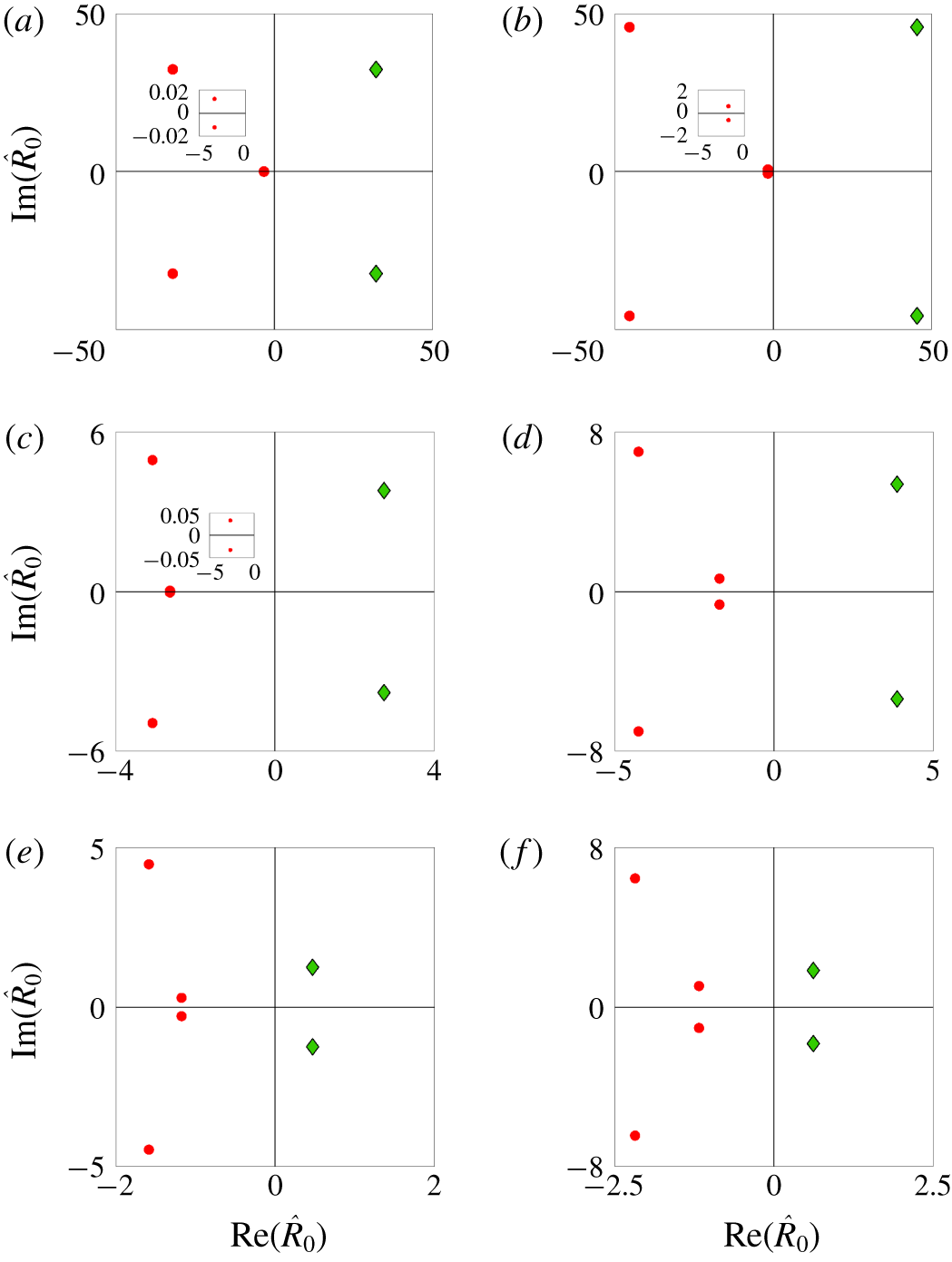
 $La$, a finite number of roots are found by numerically solving (3.23) in Matlab (MATLAB 2018) using fsolve (script file provided as additional supplementary material). Among these roots, a single conjugate pair is found to satisfy the constraint
 $\text{Re}(\hat{R}_{0})>0$ (see discussion above equation (3.10) for
 $\text{Re}(l)>0$ which translates non-dimensionally to
 $\text{Re}(\hat{R}_{0})>0$). This is shown on the complex
 $\hat{R}_{0}$ plane in figure 2(a–f) for various
 $m$ and
 $La$.
Roots of (3.23) on the complex  $\hat{R}_{0}$ plane for various
 $m$ and
 $La$. Roots in red do not satisfy the constraint
 $\text{Re}(\hat{R}_{0})>0$; (a)
 $m=2$,
 $La=7.2\times 10^{5}$, (b)
 $m=3$,
 $La=7.2\times 10^{5}$, (c)
 $m=2$,
 $La=10^{2}$, (d)
 $m=3$,
 $La=10^{2}$, (e)
 $m=2$,
 $La=2.5$, (f)
 $m=3$,
 $La=2.5$.

For all values of  $La$ and
 $m$ examined here, we numerically find a single conjugate pair of roots satisfying the constraint
 $\text{Re}(\hat{R}_{0})>0$ (roots in green in figure 2a–f). From this pair and using the relation
 $\unicode[STIX]{x1D70E}=\unicode[STIX]{x1D708}(\hat{R}_{0}/R_{0})^{2}$, we obtain a corresponding conjugate pair of values for
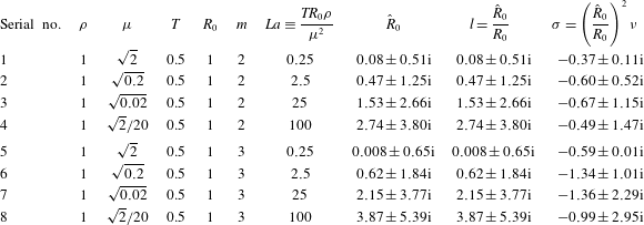
 $\unicode[STIX]{x1D70E}$. Table 1 provides a sample list of such pairs.
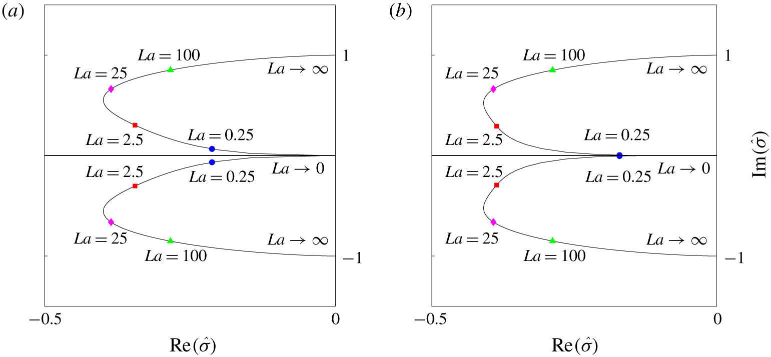
Values of  $\hat{\unicode[STIX]{x1D70E}}\equiv (\unicode[STIX]{x1D70E}/\unicode[STIX]{x1D714}_{0})$ on the complex plane for various values of
 $La$ and (a)
 $m=2$ (b)
 $m=3$.

Sample roots of (3.23) satisfying  $\text{Re}(\hat{R}_{0})>0$.

In figures 3(a) and 3(b), we show such complex conjugate pairs of values of  $\hat{\unicode[STIX]{x1D70E}}\equiv \unicode[STIX]{x1D70E}/\unicode[STIX]{x1D714}_{0}$ as a function of
 $La$ for
 $m=2$ and
 $3$, respectively. It is seen that
 $\text{Re}\left(\hat{\unicode[STIX]{x1D70E}}\right)$ is always negative implying that all perturbations are damped. For
 $La\rightarrow \infty$, the curves representing the locus of all pairs of roots start from
 $\unicode[STIX]{x1D70E}=\pm \text{i}\unicode[STIX]{x1D714}_{0}$ (given by (1.2)) and with decreasing Laplace number the curves turn around touching the
 $x$ axis asymptotically as
 $La\rightarrow 0$. This is verified from (3.23) where for
 $La=0$,
 $\hat{R}_{0}=0$ is a root of the equation. As the curves in figures 3(a) and 3(b) do not touch the real axis for any non-zero value of
 $La$, this implies that the response of the filament always remains underdamped. Such lack of overdamped behaviour has also been reported earlier for capillary oscillations on a bubble (Prosperetti Reference Prosperetti1980b). This analytical prediction of the lack of an overdamped response at large viscosity (i.e. small Laplace number) is tested using DNS in § 5.
3.2 Normal modes – continuous spectrum
In the previous section, we have numerically found that for a given value of  $m$ and
 $La$, the dispersion relation (3.23) allows only two values of
 $l$ and, correspondingly,
 $\unicode[STIX]{x1D70E}$ (a complex conjugate pair). This complex conjugate pair leads to two vorticity eigenfunctions viz. the real and the imaginary parts of
 $\text{K}_{m}(lr)$. These constitute the discrete spectrum (DS) eigenmodes. It is clear that these two eigenfunctions which decay exponentially at large radii, cannot adequately express far field vorticity perturbations. In order to ensure completeness, we need another set of eigenfunctions. We show here that (for the same
 $m$ and
 $La$ as above) there is an additional, uncountably infinite set of eigenfunctions labelled as the continuous spectrum (CS). Note that in the previous section, we had assumed that
 $\text{Re}(l)>0$. We now allow for
 $\text{Re}(l)=0$ in our analysis writing
 $l=\sqrt{\unicode[STIX]{x1D70E}/\unicode[STIX]{x1D708}}\equiv \text{i}\unicode[STIX]{x1D709}$ with
 $\unicode[STIX]{x1D709}\in \mathbb{R}^{+}$ (see Lamb (Reference Lamb1993) for a similar argument in Cartesian geometry). This implies
 $\unicode[STIX]{x1D70E}$ is a real (negative) number in contrast to earlier analysis where it was complex. We thus set
 $$\begin{eqnarray}\displaystyle & \displaystyle \unicode[STIX]{x1D702}(\unicode[STIX]{x1D703},t)=a_{0}\exp (\unicode[STIX]{x1D70E}t)\cos (m\unicode[STIX]{x1D703}), & \displaystyle\end{eqnarray}$$
 $$\begin{eqnarray}\displaystyle & \displaystyle \unicode[STIX]{x1D714}(r,\unicode[STIX]{x1D703},t)=\exp (\unicode[STIX]{x1D70E}t)\sin (m\unicode[STIX]{x1D703})\unicode[STIX]{x1D6FA}(r), & \displaystyle\end{eqnarray}$$
 $$\begin{eqnarray}\displaystyle & \displaystyle \unicode[STIX]{x1D713}(r,\unicode[STIX]{x1D703},t)=\exp (\unicode[STIX]{x1D70E}t)\sin (m\unicode[STIX]{x1D703})\unicode[STIX]{x1D6F9}(r), & \displaystyle\end{eqnarray}$$
 $$\begin{eqnarray}\displaystyle & \displaystyle p(r,\unicode[STIX]{x1D703},t)=\exp (\unicode[STIX]{x1D70E}t)\cos (m\unicode[STIX]{x1D703}){\mathcal{P}}(r), & \displaystyle\end{eqnarray}$$
and replace  $\unicode[STIX]{x1D70E}$ in the subsequent algebra with
 $-\unicode[STIX]{x1D708}\unicode[STIX]{x1D709}^{2}$. In order to avoid a profusion of symbols in the analysis, we retain the same symbols for all variables and constants of integration as in the previous section. In terms of
 $\unicode[STIX]{x1D709}$, equations (3.7) and (3.8) may be written as
 $$\begin{eqnarray}\displaystyle \frac{\text{d}^{2}\unicode[STIX]{x1D6FA}}{\text{d}r^{2}}+\frac{1}{r}\frac{\text{d}\unicode[STIX]{x1D6FA}}{\text{d}r}+\left(\unicode[STIX]{x1D709}^{2}-\frac{m^{2}}{r^{2}}\right)\unicode[STIX]{x1D6FA}=0,\quad \frac{\text{d}^{2}\unicode[STIX]{x1D6F9}}{\text{d}r^{2}}+\frac{1}{r}\frac{\text{d}\unicode[STIX]{x1D6F9}}{\text{d}r}-\frac{m^{2}}{r^{2}}\unicode[STIX]{x1D6F9}=\unicode[STIX]{x1D6FA}, & & \displaystyle\end{eqnarray}$$
respectively. The solution to the first equation in (3.28) is
 $$\begin{eqnarray}\displaystyle \unicode[STIX]{x1D6FA}(r)={\mathcal{C}}\text{J}_{m}(\unicode[STIX]{x1D709}r)+{\mathcal{D}}\text{Y}_{m}(\unicode[STIX]{x1D709}r), & & \displaystyle\end{eqnarray}$$
where  ${\mathcal{C}},{\mathcal{D}}$ are real constants of integration (as coefficients of equation (3.24) are real) and
 $\text{J}_{m},\text{Y}_{m}$ are Bessel functions of the first and second kind, respectively.
Both  $\text{J}_{m}$ and
 $\text{Y}_{m}$ decay to zero as
 $r\rightarrow \infty$, and thus unlike the discrete spectrum analysis, it is not necessary to set
 ${\mathcal{C}}$ or
 ${\mathcal{D}}$ to zero in (3.29). The solution to the second equation in (3.28) with
 $\unicode[STIX]{x1D6FA}(r)$ from (3.29) can be obtained using steps which are identical to the previous section. The detailed algebra is provided in the supplementary material. The expression for
 $\unicode[STIX]{x1D6F9}(r)$ satisfying boundedness constraints at
 $r\rightarrow \infty$ is
 $$\begin{eqnarray}\displaystyle \unicode[STIX]{x1D6F9}(r)=\unicode[STIX]{x1D6FD}r^{-m}-\frac{1}{\unicode[STIX]{x1D709}^{2}}\{{\mathcal{C}}\text{J}_{m}(\hat{r})+{\mathcal{D}}\text{Y}_{m}(\hat{r})\}+\frac{R_{0}}{2m\unicode[STIX]{x1D709}}\{{\mathcal{C}}\text{J}_{m+1}(\hat{R}_{0})+{\mathcal{D}}\text{Y}_{m+1}(\hat{R}_{0})\}\left(\frac{R_{0}}{r}\right)^{m}, & & \displaystyle \nonumber\\ \displaystyle & & \displaystyle\end{eqnarray}$$
where  $\hat{r}\equiv \unicode[STIX]{x1D709}r,\hat{R}_{0}=\unicode[STIX]{x1D709}R_{0}$. The expression for pressure is obtained by integrating the radial component of the momentum equation. After some algebra we obtain,
 $$\begin{eqnarray}\displaystyle {\mathcal{P}}(r)=\unicode[STIX]{x1D70C}\left[\unicode[STIX]{x1D708}\unicode[STIX]{x1D709}^{2}\unicode[STIX]{x1D6FD}r^{-m}+\frac{\unicode[STIX]{x1D708}\hat{R}_{0}}{2m}\{{\mathcal{C}}\text{J}_{m+1}(\hat{R}_{0})+{\mathcal{D}}\text{Y}_{m+1}(\hat{R}_{0})\}\left(\frac{R_{0}}{r}\right)^{m}\right]. & & \displaystyle\end{eqnarray}$$
Note that we now have four unknowns viz.  ${\mathcal{C}},{\mathcal{D}},a_{0}$ and
 $\unicode[STIX]{x1D6FD}$ with three boundary conditions (like earlier) to determine these. Substituting expressions (3.24)–(3.27) into (2.11)–(2.13) and using expressions for
 $\unicode[STIX]{x1D6FA}(r),\unicode[STIX]{x1D6F9}(r)$ and
 ${\mathcal{P}}(r)$ from (3.29), (3.30) and (3.31), respectively, we obtain the following linear equations. Due to having three equations for four unknowns (
 $a_{0},\unicode[STIX]{x1D6FD},{\mathcal{C}},{\mathcal{D}}$), we can only determine three ratios from these equations. We have chosen these to be
 $a_{0}/\unicode[STIX]{x1D6FD},{\mathcal{C}}/\unicode[STIX]{x1D6FD}$ and
 ${\mathcal{D}}/\unicode[STIX]{x1D6FD}$. The equations for these are,
 $$\begin{eqnarray}\displaystyle & \displaystyle a_{11}\left(\frac{a_{0}}{\unicode[STIX]{x1D6FD}}\right)+a_{12}\left(\frac{{\mathcal{C}}}{\unicode[STIX]{x1D6FD}}\right)+a_{13}\left(\frac{{\mathcal{D}}}{\unicode[STIX]{x1D6FD}}\right)=-mR_{0}^{-m-1}, & \displaystyle\end{eqnarray}$$
 $$\begin{eqnarray}\displaystyle & \displaystyle a_{21}\left(\frac{a_{0}}{\unicode[STIX]{x1D6FD}}\right)+a_{22}\left(\frac{{\mathcal{C}}}{\unicode[STIX]{x1D6FD}}\right)+a_{23}\left(\frac{{\mathcal{D}}}{\unicode[STIX]{x1D6FD}}\right)=2m(m+1)R_{0}^{-m-2}, & \displaystyle\end{eqnarray}$$
 $$\begin{eqnarray}\displaystyle & \displaystyle a_{31}\left(\frac{a_{0}}{\unicode[STIX]{x1D6FD}}\right)+a_{32}\left(\frac{{\mathcal{C}}}{\unicode[STIX]{x1D6FD}}\right)+a_{33}\left(\frac{{\mathcal{D}}}{\unicode[STIX]{x1D6FD}}\right)=-\unicode[STIX]{x1D708}\unicode[STIX]{x1D709}^{2}R_{0}^{-m}\left(1-\frac{2m(m+1)}{\hat{R}_{0}^{2}}\right), & \displaystyle\end{eqnarray}$$
with the coefficients
 $$\begin{eqnarray}\displaystyle \left.\begin{array}{@{}c@{}}\displaystyle a_{11}\equiv -\unicode[STIX]{x1D708}\unicode[STIX]{x1D709}^{2},\quad a_{12}\equiv \frac{1}{\unicode[STIX]{x1D709}}\left\{\frac{1}{2}\text{J}_{m+1}(\hat{R}_{0})-\frac{m}{\hat{R}_{0}}\text{J}_{m}(\hat{R}_{0})\right\},\\ \displaystyle a_{13}\equiv \frac{1}{\unicode[STIX]{x1D709}}\left\{\frac{1}{2}\text{Y}_{m+1}(\hat{R}_{0})-\frac{m}{\hat{R}_{0}}\text{Y}_{m}(\hat{R}_{0})\right\},\\ \displaystyle a_{21}\equiv 0,\quad a_{22}\equiv \text{J}_{m-1}^{\prime }(\hat{R}_{0}),\quad a_{23}\equiv \text{Y}_{m-1}^{\prime }(\hat{R}_{0}),\\ \displaystyle a_{31}\equiv -\frac{T}{\unicode[STIX]{x1D70C}R_{0}^{2}}(1-m^{2}),\quad a_{32}\equiv \frac{\unicode[STIX]{x1D708}}{\hat{R}_{0}}\left[\frac{\hat{R}_{0}^{2}}{2m}\text{J}_{m+1}(\hat{R}_{0})-(m-1)\text{J}_{m-1}(\hat{R}_{0})\right],\\ \displaystyle a_{33}\equiv \frac{\unicode[STIX]{x1D708}}{\hat{R}_{0}}\left[\frac{\hat{R}_{0}^{2}}{2m}\text{Y}_{m+1}(\hat{R}_{0})-(m-1)\text{Y}_{m-1}(\hat{R}_{0})\right].\end{array}\right\} & & \displaystyle\end{eqnarray}$$
In contrast to the analysis in § 3.1, note that equations (3.32)–(3.34) are three inhomogeneous equations. It is clear that there is no dispersion relation in the present case, since the determinant of the homogenous part of (3.32)–(3.34) is not zero in order to obtain a non-trivial solution. Non-trivial values of  $(a_{0}/\unicode[STIX]{x1D6FD},{\mathcal{C}}/\unicode[STIX]{x1D6FD},{\mathcal{D}}/\unicode[STIX]{x1D6FD})$ are obtainable for every value of
 $0<\unicode[STIX]{x1D709}<\infty$ by solving equations (3.32)–(3.34). Note that since
 $\unicode[STIX]{x1D70E}=-\unicode[STIX]{x1D708}\unicode[STIX]{x1D709}^{2}$, this implies that
 $-\infty <\unicode[STIX]{x1D70E}<0$ for the continuous spectrum.
3.3 Eigenfunctions and completeness
Having demonstrated the existence of the discrete and continuous spectrum in §§ 3.1 and 3.2, we now examine the vorticity eigenfunctions. For a given value of  $m$ and
 $La$, there is a complex conjugate pair of
 $l,\bar{l}$ obtained from the dispersion relation and correspondingly the DS eigenmodes for vorticity are (equation (3.9) with
 ${\mathcal{D}}=0$)
 $$\begin{eqnarray}\displaystyle \text{K}_{m}(lr),\quad \text{K}_{m}(\bar{l}r). & & \displaystyle\end{eqnarray}$$
These modes decay to zero exponentially fast as  $r\rightarrow \infty$ since
 $\text{K}_{m}(z)\sim \sqrt{\unicode[STIX]{x03C0}/2z}\exp (-z)$ as
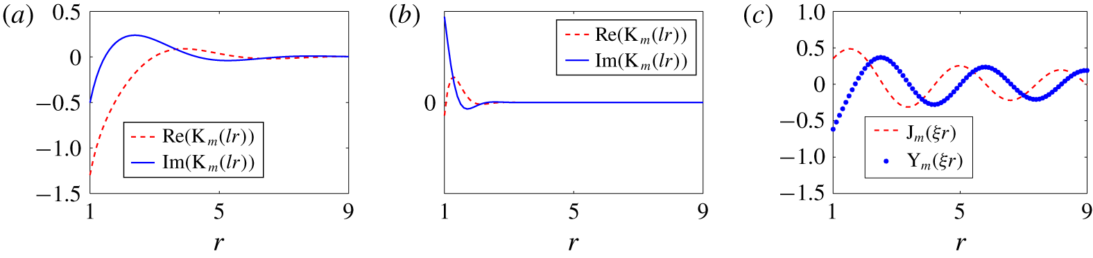
 $z\rightarrow \infty$. Figure 4(a,b) shows these eigenfunctions plotted as a function of radius for two different values of
 $La$. It is seen that the length scale of decay of the eigenmodes increases with increasing viscosity. In addition we also have the CS eigenmodes which decay algebraically to zero. These are (equation (3.29))
 $$\begin{eqnarray}\displaystyle \text{J}_{m}(\unicode[STIX]{x1D709}r),\quad \text{Y}_{m}(\unicode[STIX]{x1D709}r), & & \displaystyle\end{eqnarray}$$
with  $0<\unicode[STIX]{x1D709}<\infty$. Note that the DS eigenfunctions in (3.36) are square integrable (in
 $R_{0}+\unicode[STIX]{x1D702}\leqslant r\leqslant \infty$) while those in (3.37) are not, in agreement with known behaviour of CS eigenfunctions in other geometries (Prosperetti Reference Prosperetti1976, Reference Prosperetti1980a; Farsoiya et al. Reference Farsoiya, Mayya and Dasgupta2017).
(a,b) DS eigenmodes. (c) CS eigenmodes, with (a)  $La=2.5,m=2$, (b)
 $La=100,m=2$, (c)
 $\unicode[STIX]{x1D709}=2$.

The completeness theorem (for the perturbation vorticity field) may be written as a linear superposition of the DS and the CS modes. For an interfacial Fourier mode of index  $m$, any arbitrary initial distribution of vorticity may be (formally) represented as
 $$\begin{eqnarray}\displaystyle \unicode[STIX]{x1D6FA}(r,0)=\mathop{\sum }_{i}C_{i}\text{K}_{m}(l^{(i)}r)+\int _{0}^{\infty }\{D(\unicode[STIX]{x1D709})\text{J}_{m}(\unicode[STIX]{x1D709}r)+E(\unicode[STIX]{x1D709})\text{Y}_{m}(\unicode[STIX]{x1D709}r)\}\unicode[STIX]{x1D709}\,\text{d}\unicode[STIX]{x1D709}, & & \displaystyle\end{eqnarray}$$
where  $C_{i},D(\unicode[STIX]{x1D709})$ and
 $E(\unicode[STIX]{x1D709})$ are to be obtained from the inner product of
 $\unicode[STIX]{x1D6FA}(r,0)$ with
 $\text{K}_{m}$,
 $\text{J}_{m}$ and
 $\text{Y}_{m}$ using suitable orthogonality conditions. The integral in (3.38) is purposely written in the form of an inverse Fourier–Bessel transform. From normal mode analysis, the time evolution of
 $\unicode[STIX]{x1D6FA}(r,t)$ may be written as
 $$\begin{eqnarray}\displaystyle \unicode[STIX]{x1D6FA}(r,t) & = & \displaystyle \mathop{\sum }_{i}C_{i}\text{K}_{m}(l^{(i)}r)\exp (\unicode[STIX]{x1D70E}^{(i)}t)\nonumber\\ \displaystyle & & \displaystyle +\,\int _{0}^{\infty }\{D(\unicode[STIX]{x1D709})\text{J}_{m}(\unicode[STIX]{x1D709}r)+E(\unicode[STIX]{x1D709})\text{Y}_{m}(\unicode[STIX]{x1D709}r)\}\unicode[STIX]{x1D709}\exp (-\unicode[STIX]{x1D708}\unicode[STIX]{x1D709}^{2}t)\,\text{d}\unicode[STIX]{x1D709},\end{eqnarray}$$
where it is seen that (3.38) is recovered from (3.39) at  $t=0$. The integral in (3.39) can produce terms with non-exponential time dependence, a contribution which is missed if the continuous spectrum is not taken into account. It will be seen in the next section, that perturbing the interface with a single Fourier mode and zero perturbation vorticity everywhere in space, represents such an initial condition.
Similar to (3.38) which is a decomposition in space, it is also possible to write a corresponding completeness theorem for any function of time by expressing it as a linear combination of the discrete spectrum frequencies (allowed by the dispersion relation) and an integral superposition over the continuous spectrum frequencies e.g. the amplitude of the standing wave perturbation is expected to be
 $$\begin{eqnarray}\displaystyle \frac{a(t)}{a_{0}}=\mathop{\sum }_{i}\unicode[STIX]{x1D705}_{i}\exp (\unicode[STIX]{x1D70E}^{(i)}t)+\int _{-\infty }^{0}\unicode[STIX]{x1D6EF}(\unicode[STIX]{x1D70E})\exp (\unicode[STIX]{x1D70E}t)\,\text{d}\unicode[STIX]{x1D70E}, & & \displaystyle\end{eqnarray}$$
where  $\unicode[STIX]{x1D705}_{i}$ and
 $\unicode[STIX]{x1D6EF}(\unicode[STIX]{x1D70E})$ are to be obtained from the initial conditions. Note that the
 $\unicode[STIX]{x1D70E}_{i}$ in (3.39) and (3.40) are obtained from the
 $l^{(i)}$ using the relation
 $\unicode[STIX]{x1D70E}^{(i)}=\unicode[STIX]{x1D708}(l^{(i)})^{2}$ ensuring that only those
 $l^{(i)}$ satisfying
 $\text{Re}(l^{(i)})>0$ are used. Equations (3.39) and (3.40) are written based on the normal mode analysis presented here and in § 3.1. By solving the corresponding IVP, it will be shown in § 4 that one can analytically obtain expressions of exactly the same form as (3.39) and (3.40). Furthermore, the IVP solution will provide expressions for
 $C_{i},D(\unicode[STIX]{x1D709}),E(\unicode[STIX]{x1D709})$ in (3.39) as well as
 $\unicode[STIX]{x1D705}_{i},\unicode[STIX]{x1D6EF}(\unicode[STIX]{x1D70E})$ in (3.40).
4 Initial value problem
In this section, we solve the IVP with initial perturbation comprising a single interfacial azimuthal Fourier mode of index  $m$ with zero initial velocity (vorticity) everywhere in the outer fluid. We further assume that there is no impulse at the interface initially. For
 $m\geqslant 2$ and
 $La>0$, it is seen from (3.36) and (3.37) that the vorticity field associated with the DS and CS eigenfunctions decays to zero exponentially and algebraically, respectively. Consequently the aforementioned initial condition we solve for here, requires a linear superposition of the DS as well as the CS eigenfunctions, to achieve a cancellation of vorticity everywhere in space. This implies that the initial condition excites the DS and the CS modes. We consequently anticipate the temporal evolution of the interface to be a summation of discrete exponential terms and an integral over a continuous range of exponential terms (see Prosperetti (Reference Prosperetti1976) for similar conclusions for viscous capillary waves on a deep pool of liquid). For solving the IVP, we set
 $$\begin{eqnarray}\displaystyle & \displaystyle \unicode[STIX]{x1D702}(\unicode[STIX]{x1D703},t)=a(t)\cos (m\unicode[STIX]{x1D703}), & \displaystyle\end{eqnarray}$$
 $$\begin{eqnarray}\displaystyle & \displaystyle \unicode[STIX]{x1D714}(r,\unicode[STIX]{x1D703},t)=\sin (m\unicode[STIX]{x1D703})\unicode[STIX]{x1D6FA}(r,t), & \displaystyle\end{eqnarray}$$
 $$\begin{eqnarray}\displaystyle & \displaystyle \unicode[STIX]{x1D713}(r,\unicode[STIX]{x1D703},t)=\sin (m\unicode[STIX]{x1D703})\unicode[STIX]{x1D6F9}(r,t), & \displaystyle\end{eqnarray}$$
 $$\begin{eqnarray}\displaystyle & \displaystyle p(r,\unicode[STIX]{x1D703},t)=\cos (m\unicode[STIX]{x1D703}){\mathcal{P}}(r,t). & \displaystyle\end{eqnarray}$$
Substituting expressions (4.1)–(4.4) in (2.5) and (2.6), we obtain
 $$\begin{eqnarray}\displaystyle & \displaystyle \frac{\unicode[STIX]{x2202}\unicode[STIX]{x1D6FA}}{\unicode[STIX]{x2202}t}=\unicode[STIX]{x1D708}\left[\frac{\unicode[STIX]{x2202}^{2}\unicode[STIX]{x1D6FA}}{\unicode[STIX]{x2202}r^{2}}+\frac{1}{r}\frac{\unicode[STIX]{x2202}\unicode[STIX]{x1D6FA}}{\unicode[STIX]{x2202}r}-\frac{m^{2}}{r^{2}}\unicode[STIX]{x1D6FA}\right], & \displaystyle\end{eqnarray}$$
 $$\begin{eqnarray}\displaystyle & \displaystyle \frac{\unicode[STIX]{x2202}^{2}\unicode[STIX]{x1D6F9}}{\unicode[STIX]{x2202}r^{2}}+\frac{1}{r}\frac{\unicode[STIX]{x2202}\unicode[STIX]{x1D6F9}}{\unicode[STIX]{x2202}r}-\frac{m^{2}}{r^{2}}\unicode[STIX]{x1D6F9}=\unicode[STIX]{x1D6FA}. & \displaystyle\end{eqnarray}$$
Define the Laplace transform and inverse transform pair  $f(t)$ and
 $\tilde{f}(s)$ as,
 $$\begin{eqnarray}\displaystyle \tilde{f}(s)\equiv \int _{0}^{\infty }f(t)\exp (-st)\,\text{d}t. & & \displaystyle\end{eqnarray}$$
With initial conditions described earlier in this section, we have  $a(0)=a_{0}$,
 ${\dot{a}}(0)=0$,
 $\unicode[STIX]{x1D6FA}(r,0)=0$ and the Laplace transform of (4.5) and (4.6) is (Laplace transformed variables are indicated with a tilde on top)
 $$\begin{eqnarray}\displaystyle \frac{\unicode[STIX]{x2202}^{2}\tilde{\unicode[STIX]{x1D6FA}}}{\unicode[STIX]{x2202}r^{2}}+\frac{1}{r}\frac{\unicode[STIX]{x2202}\tilde{\unicode[STIX]{x1D6FA}}}{\unicode[STIX]{x2202}r}-\left(\frac{s}{\unicode[STIX]{x1D708}}+\frac{m^{2}}{r^{2}}\right)\tilde{\unicode[STIX]{x1D6FA}}=0,\quad \frac{\unicode[STIX]{x2202}^{2}\tilde{\unicode[STIX]{x1D6F9}}}{\unicode[STIX]{x2202}r^{2}}+\frac{1}{r}\frac{\unicode[STIX]{x2202}\tilde{\unicode[STIX]{x1D6F9}}}{\unicode[STIX]{x2202}r}-\frac{m^{2}}{r^{2}}\tilde{\unicode[STIX]{x1D6F9}}=\tilde{\unicode[STIX]{x1D6FA}}(r,s). & & \displaystyle\end{eqnarray}$$
The algebra henceforth is entirely similar to that in § 3.1 except that now (4.5) and (4.6) are partial differential equations. The solutions to the first and second equation in (4.8) are
 $$\begin{eqnarray}\displaystyle & \displaystyle \tilde{\unicode[STIX]{x1D6FA}}(r,s)=\tilde{{\mathcal{C}}}(s)\text{K}_{m}(hr), & \displaystyle\end{eqnarray}$$
 $$\begin{eqnarray}\displaystyle & \displaystyle \tilde{\unicode[STIX]{x1D6F9}}(r,s)=\tilde{\unicode[STIX]{x1D6FD}}(s)r^{-m}+\left(\frac{\tilde{{\mathcal{C}}}(s)}{h^{2}}\right)\text{K}_{m}(hr)-\frac{\tilde{{\mathcal{C}}}(s)R_{0}}{2mh}\left(\frac{r}{R_{0}}\right)^{-m}\text{K}_{m+1}(hR_{0}), & \displaystyle\end{eqnarray}$$
where  $h\equiv \sqrt{s/\unicode[STIX]{x1D708}}$.
 $\tilde{{\mathcal{C}}}(s),\tilde{{\mathcal{D}}}(s)$ are complex functions while
 $\unicode[STIX]{x1D6FD}(s)$ is a real function of
 $s$. Equations (4.9) and (4.10) are obtained under the constraint
 $\text{Re}\left(h\right)>0$ in order to prevent divergence as
 $r\rightarrow \infty$. We discuss this point when discussing the Laplace inversion in appendix D. Using steps identical to the discrete spectrum derivation, we can obtain an expression for the radial part of the perturbation pressure in the Laplace domain. This is,
 $$\begin{eqnarray}\displaystyle \tilde{{\mathcal{P}}}(r,s)=\unicode[STIX]{x1D70C}\left\{-s\tilde{\unicode[STIX]{x1D6FD}}(s)r^{-m}+\frac{s\tilde{{\mathcal{C}}}(s)R_{0}}{2mh}\left(\frac{r}{R_{0}}\right)^{-m}\text{K}_{m+1}(hR_{0})\right\}. & & \displaystyle\end{eqnarray}$$
Laplace transforming the boundary conditions (2.11)–(2.13) and using expressions for  $\tilde{\unicode[STIX]{x1D6FA}}(r,s),\tilde{\unicode[STIX]{x1D6F9}}(r,s)$ and
 $\tilde{{\mathcal{P}}}(r,s)$ from (4.9)–(4.11) in these, we obtain three inhomogenous equations in the three unknowns viz.
 $\tilde{a}_{m}(s),\tilde{{\mathcal{C}}}(s)$ and
 $\tilde{\unicode[STIX]{x1D6FD}}(s)$. These are
 $$\begin{eqnarray}\displaystyle & \displaystyle \frac{s}{R_{0}}\tilde{a}(s)-\frac{\text{K}_{m-1}(hR_{0})}{2hR_{0}}\tilde{{\mathcal{C}}}(s)+mR_{0}^{-m-2}\tilde{\unicode[STIX]{x1D6FD}}(s)=\frac{a_{0}}{R_{0}}, & \displaystyle\end{eqnarray}$$
 $$\begin{eqnarray}\displaystyle & \displaystyle -\text{K}_{m-1}^{\prime }(hR_{0})\;\tilde{{\mathcal{C}}}(s)+2m(m+1)R_{0}^{-m-2}\tilde{\unicode[STIX]{x1D6FD}}(s)=0, & \displaystyle\end{eqnarray}$$
 $$\begin{eqnarray}\displaystyle & & \displaystyle -\frac{T}{\unicode[STIX]{x1D70C}R_{0}^{2}}(1-m^{2})\tilde{a}(s)+\frac{\unicode[STIX]{x1D708}}{hR_{0}}\left[\frac{h^{2}R_{0}^{2}}{2m}\text{K}_{m+1}(hR_{0})-(m-1)\text{K}_{m-1}(hR_{0})\right]\tilde{{\mathcal{C}}}(s)\nonumber\\ \displaystyle & & \displaystyle \qquad -\,sR_{0}^{-m}\left(1+\frac{2m(m+1)}{h^{2}R_{0}^{2}}\right)\tilde{\unicode[STIX]{x1D6FD}}(s)=0.\end{eqnarray}$$
The expression for  $\tilde{a}(s)$ can be obtained from (4.12)–(4.14). It is shown in § 3 of the supplementary material that this is (written in the same form as by Prosperetti (Reference Prosperetti1976) earlier in Cartesian geometry),
 $$\begin{eqnarray}\displaystyle \tilde{a}(s)=\left[\frac{s+{\mathcal{M}}(s)}{s^{2}+s{\mathcal{M}}(s)+w_{0}^{2}\unicode[STIX]{x1D712}(s)}\right]a_{0},\quad \text{Re}\left(\sqrt{\frac{s}{\unicode[STIX]{x1D708}}}\right)>0, & & \displaystyle\end{eqnarray}$$
with
 $$\begin{eqnarray}\displaystyle \left.\begin{array}{@{}c@{}}\displaystyle {\mathcal{G}}(s)\equiv {\displaystyle \frac{{\displaystyle \frac{s}{\unicode[STIX]{x1D708}}}R_{0}^{2}}{2m}}\text{K}_{m+1}\left(\sqrt{\frac{s}{\unicode[STIX]{x1D708}}}R_{0}\right)-(m-1)\text{K}_{m-1}\left(\sqrt{\frac{s}{\unicode[STIX]{x1D708}}}R_{0}\right),\\ \displaystyle \unicode[STIX]{x1D712}(s)\equiv 1-\frac{(m+1)}{\sqrt{{\displaystyle \frac{s}{\unicode[STIX]{x1D708}}}}R_{0}}\frac{\text{K}_{m-1}\left(\sqrt{{\displaystyle \frac{s}{\unicode[STIX]{x1D708}}}}R_{0}\right)}{\text{K}_{m-1}^{\prime }\left(\sqrt{{\displaystyle \frac{s}{\unicode[STIX]{x1D708}}}}R_{0}\right)},\\ \displaystyle {\mathcal{M}}(s)\equiv {\displaystyle \frac{2\unicode[STIX]{x1D708}m(m+1)}{R_{0}^{2}}}\left(1-{\displaystyle \frac{{\mathcal{G}}(s)}{\sqrt{{\displaystyle \frac{s}{\unicode[STIX]{x1D708}}}}R_{0}\text{K}_{m-1}^{\prime }\left(\sqrt{{\displaystyle \frac{s}{\unicode[STIX]{x1D708}}}}R_{0}\right)}}\right),\\ \displaystyle w_{0}^{2}\equiv \frac{Tm(m^{2}-1)}{\unicode[STIX]{x1D70C}R_{0}^{3}}.\end{array}\right\} & & \displaystyle\end{eqnarray}$$
Note that  $\unicode[STIX]{x1D714}_{0}$ is the inviscid frequency discussed in the Introduction in (1.2), under the approximation
 $\unicode[STIX]{x1D70C}^{{\mathcal{O}}}\gg \unicode[STIX]{x1D70C}^{{\mathcal{I}}}$.
In order to obtain an expression for  $a(t)$, we need the Laplace inversion of (4.15). For this it is necessary to know the poles and branch points (and the consequent branch cut structure) of
 $\tilde{a}(s)$. The possibility of
 $\tilde{a}(s)$ having branch points arises due to
 $\text{K}_{m}(z)$ having a branch point at
 $z=0$ (and at
 $z=\infty$) (Abramowitz & Stegun Reference Abramowitz and Stegun1965) as seen from the following series representation (Parnes Reference Parnes1972):
 $$\begin{eqnarray}\displaystyle \text{K}_{m}(z) & = & \displaystyle \frac{1}{2}\mathop{\sum }_{r=0}^{m-1}(-1)^{r}\frac{(m-r-1)!}{r!}\left(\frac{2}{z}\right)^{m-2r}\nonumber\\ \displaystyle & & \displaystyle +\,(-1)^{m+1}\frac{1}{m!}\left(\frac{z}{2}\right)^{m}\left[\ln \left(\frac{z}{2}\right)-\frac{1}{2}\unicode[STIX]{x1D6F9}(m+1)+\frac{1}{2}\unicode[STIX]{x1D6FE}\right]+\cdots \,,\end{eqnarray}$$
where  $\unicode[STIX]{x1D6F9}(m+1)=1+\frac{1}{2}+\frac{1}{3}+\cdots +1/m-\unicode[STIX]{x1D6FE}$ and
 $\unicode[STIX]{x1D6FE}\approx 0.57721$ is the Euler–Mascheroni constant and
 $\unicode[STIX]{x1D6F9}(1)=-\unicode[STIX]{x1D6FE}$. Expression (4.17) evaluated for specific cases of
 $m=1,2,3$ and
 $4$ are provided in the additional supplementary material. It is clear from these expressions that for
 $m>0$,
 $\text{K}_{m}(z)$ diverges as
 $z^{-m}$ at
 $z=0$ and in addition
 $z=0$ is also a logarithmic branch point. In order to show that
 $\tilde{a}(s)$ in (4.15) has a branch point at
 $s=0$, we use the Series function in Mathematica (Wolfram Research, Inc. 2016) and expand
 $\tilde{a}(s)$ for
 $m=2,3$ etc. To prevent lengthy expressions we set
 $\unicode[STIX]{x1D707}=\sqrt{0.2}$,
 $R_{0}=1.0$,
 $T=0.5$,
 $\unicode[STIX]{x1D70C}=1$ with
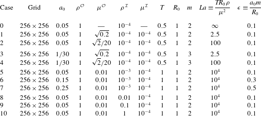
 $m=2,3$ in (4.15) (these parameters correspond to cases
 $1$ and
 $3$ in table 2 described in § 5) for obtaining these expansions, although the conclusions are expected to remain true for other values as well. The expansions are (subscripts on
 $\tilde{a}(s)$ indicate the value of
 $m$)
 $$\begin{eqnarray}\displaystyle \frac{\tilde{a}_{2}(s)}{a_{0}}=0.894427+(-0.75\ln (s)-0.896309)s+\cdots \,, & & \displaystyle\end{eqnarray}$$
 $$\begin{eqnarray}\displaystyle \begin{array}{@{}rcl@{}}\displaystyle \frac{\tilde{a}_{3}(s)}{a_{0}}\ & =\ & 0.596285-0.05s+(0.124226\ln (s)-0.122629)s^{2}+\cdots \,,\\ \displaystyle \vdots \!\!\ & \ & \!\!\vdots \!\quad \quad \qquad \vdots \!\quad \quad \qquad \vdots \!\quad \quad \qquad \vdots \!\quad \quad \qquad \vdots \!\quad \quad \qquad \vdots \!\quad \quad \qquad \vdots \end{array} & & \displaystyle\end{eqnarray}$$
Note the presence of terms of the form  $s^{m-1}\ln (s)$ in (4.18) and (4.19) which have branch points at
 $s=0$ and
 $s=\infty$. These branch points are inherited from
 $\text{K}_{m}(\sqrt{s/\unicode[STIX]{x1D708}}R_{0})$ as can be seen in the series expansions provided in the supplementary material. We depict the imaginary parts of
 $\tilde{a}(s)$ given by (4.15) for
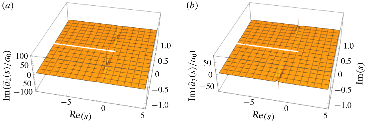
 $m=2,3$ in figures 5(a) and 5(b). It is clearly seen that the negative real axis is a line of discontinuity for
 $\text{Im}(\tilde{a}(s)/a_{0})$ for
 $m=2$ and
 $3$, respectively. The peaks in these figures are due to the two poles of
 $\tilde{a}(s)$ and the domain of the imaginary axis (
 $\text{Im}(s)$) has been restricted to enable visualisation of the branch cut.
Discontinuity of  $\text{Im}(\tilde{a}(s))$ in (4.15) on the negative real axis, for
 $m=2$ and
 $3$. The peaks are due to the poles of
 $\tilde{a}_{2}(s)$ and
 $\tilde{a}_{3}(s)$. Parameters for
 $\tilde{a}(s)$ have been chosen corresponding to case
 $1$ and
 $3$ in table 2; (a)
 $\text{Im}(\tilde{a}_{2}(s)/a_{0})$ on complex
 $s$ plane, (b)
 $\text{Im}(\tilde{a}_{3}(s)/a_{0})$ on complex
 $s$ plane.

The DNS parameters.

We now proceed to invert (4.15) for which we re-write it as,
 $$\begin{eqnarray}\displaystyle \tilde{a}(s)=\frac{{\mathcal{L}}(s)}{{\mathcal{Q}}(s)}a_{0},\quad {\mathcal{Q}}(s)\equiv s^{2}+s{\mathcal{M}}(s)+\unicode[STIX]{x1D714}^{2}\unicode[STIX]{x1D712}(s),\quad {\mathcal{L}}(s)\equiv s+{\mathcal{M}}(s). & & \displaystyle\end{eqnarray}$$
As is to be expected, the denominator  ${\mathcal{Q}}(s)$ in (4.20) is the dispersion relation (3.23) written in terms of
 $\unicode[STIX]{x1D70E}$, with
 $s$ replacing
 $\unicode[STIX]{x1D70E}$. Denoting the roots of
 ${\mathcal{Q}}(s)=0$ as
 $s_{i}$ (i.e. roots satisfying the constraint
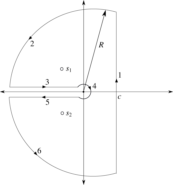
 $\text{Re}(\sqrt{s/\unicode[STIX]{x1D708}})>0$, see (4.15)) and using the Cauchy residue theorem, the formal inversion of (4.20) may be expressed as (using the keyhole contour discussed in appendix E)
 $$\begin{eqnarray}\displaystyle \frac{a(t)}{a(0)} & = & \displaystyle \frac{1}{2\unicode[STIX]{x03C0}\text{i}}\int _{c-\text{i}\infty }^{c+\text{i}\infty }\frac{{\mathcal{L}}(s)}{{\mathcal{Q}}(s)}\exp [st]\,\text{d}s\nonumber\\ \displaystyle & = & \displaystyle \mathop{\sum }_{i}\frac{{\mathcal{L}}(s_{i})}{{\mathcal{Q}}^{\prime }(s_{i})}\exp (s_{i}t)\nonumber\\ \displaystyle & & \displaystyle -\,\frac{1}{2\unicode[STIX]{x03C0}\text{i}}\int _{0}^{\infty }\left\{\left(\frac{{\mathcal{L}}(x\exp (\text{i}\unicode[STIX]{x03C0}))}{{\mathcal{Q}}(x\exp (\text{i}\unicode[STIX]{x03C0}))}\right)-\left(\frac{{\mathcal{L}}(x\exp (-\text{i}\unicode[STIX]{x03C0}))}{{\mathcal{Q}}(x\exp (-\text{i}\unicode[STIX]{x03C0}))}\right)\right\}\exp [-xt]\,\text{d}x,\qquad\end{eqnarray}$$
with  $c>0$ and the prime in
 ${\mathcal{Q}}^{\prime }$ denoting a derivative. Note that the ratio
 ${\mathcal{L}}(s)/{\mathcal{Q}}(s)$ satisfies the relation
 $$\begin{eqnarray}\displaystyle \frac{{\mathcal{L}}(\bar{s})}{{\mathcal{Q}}(\bar{s})}=\overline{\left(\frac{{\mathcal{L}}(s)}{{\mathcal{Q}}(s)}\right)}. & & \displaystyle\end{eqnarray}$$
Consequently, the expression inside the braces in the integral of (4.21) is a purely imaginary quantity implying (4.21) may be written as
 $$\begin{eqnarray}\displaystyle \frac{a(t)}{a(0)}=\mathop{\sum }_{i}\frac{{\mathcal{L}}(s_{i})}{{\mathcal{Q}}^{\prime }(s_{i})}\exp (s_{i}t)-\frac{1}{\unicode[STIX]{x03C0}}\int _{0}^{\infty }\text{Im}\left\{\left(\frac{{\mathcal{L}}(x\exp (\text{i}\unicode[STIX]{x03C0}))}{{\mathcal{Q}}(x\exp (\text{i}\unicode[STIX]{x03C0}))}\right)\right\}\exp [-xt]\,\text{d}x. & & \displaystyle\end{eqnarray}$$
Comparing (4.23) with expression (3.40), with the replacement  $\unicode[STIX]{x1D70E}=-x$, it is seen that they are the same expressions. Equation (4.23) serves to determine
 $\unicode[STIX]{x1D705}_{i}$ and
 $\unicode[STIX]{x1D6EF}(\unicode[STIX]{x1D70E})$ in (3.40). Expression (3.40) was obtained from normal mode analysis while (4.23) obtained through the IVP solution validates our analysis. In an entirely analogous manner, the inversion for
 $\tilde{\unicode[STIX]{x1D6FA}}(r,s)$ in (4.9) (see expression for
 $\tilde{C}(s)$ in appendix D) may be accomplished using the Cauchy residue theorem as
 $$\begin{eqnarray}\displaystyle \hat{\unicode[STIX]{x1D6FA}}(r,t) & \equiv & \displaystyle \frac{R_{0}}{2(m+1)a_{0}\unicode[STIX]{x1D714}_{0}^{2}}\unicode[STIX]{x1D6FA}(r,t)\nonumber\\ \displaystyle & = & \displaystyle \mathop{\sum }_{i}\frac{\text{K}_{m}\left(r\sqrt{{\displaystyle \frac{s_{i}}{\unicode[STIX]{x1D708}}}}\right)}{\text{K}_{m-1}^{\prime }\left(R_{0}\sqrt{{\displaystyle \frac{s_{i}}{\unicode[STIX]{x1D708}}}}\right){\mathcal{Q}}^{\prime }(s_{i})}\exp (s_{i}t)\nonumber\\ \displaystyle & & \displaystyle -\,\frac{1}{\unicode[STIX]{x03C0}}\int _{0}^{\infty }\text{Im}\left\{\left(\frac{{\mathcal{R}}(r,x\exp (\text{i}\unicode[STIX]{x03C0}))}{{\mathcal{Q}}(x\exp (\text{i}\unicode[STIX]{x03C0}))}\right)\right\}\exp [-xt]\,\text{d}x,\end{eqnarray}$$
with  ${\mathcal{R}}(r,s)\equiv (\text{K}_{m}(r\sqrt{s/\unicode[STIX]{x1D708}}))/(\text{K}_{m-1}^{\prime }(R_{0}\sqrt{s/\unicode[STIX]{x1D708}}))$ and the prime indicating differentiation. It is shown in appendix E that the integral on the right-hand side of (4.24) may be re-written in terms of Bessel functions
 $\text{J}$ and
 $\text{Y}$ allowing us to rewrite (4.24) as
 $$\begin{eqnarray}\displaystyle \hat{\unicode[STIX]{x1D6FA}}(r,t) & = & \displaystyle \mathop{\sum }_{i}\frac{\text{K}_{m}\left(r\sqrt{{\displaystyle \frac{s_{i}}{\unicode[STIX]{x1D708}}}}\right)}{\text{K}_{m-1}^{\prime }\left(R_{0}\sqrt{{\displaystyle \frac{s_{i}}{\unicode[STIX]{x1D708}}}}\right){\mathcal{Q}}^{\prime }(s_{i})}\exp (s_{i}t)\nonumber\\ \displaystyle & & \displaystyle -\,\frac{1}{\unicode[STIX]{x03C0}}\int _{0}^{\infty }\frac{{\mathcal{A}}(x)\text{J}_{m}\left(r\sqrt{{\displaystyle \frac{x}{\unicode[STIX]{x1D708}}}}\right)-{\mathcal{B}}(x)\text{Y}_{m}\left(r\sqrt{{\displaystyle \frac{x}{\unicode[STIX]{x1D708}}}}\right)}{{\mathcal{A}}(x)^{2}+{\mathcal{B}}(x)^{2}}\exp [-xt]\,\text{d}x,\end{eqnarray}$$
with
 $$\begin{eqnarray}\displaystyle \left.\begin{array}{@{}c@{}}\displaystyle {\mathcal{A}}(x)\equiv (x^{2}-\unicode[STIX]{x1D714}_{0}^{2})\text{Y}_{m}(\unicode[STIX]{x1D6FC})+2x^{2}\left\{\text{Y}_{m}^{\prime \prime }(\unicode[STIX]{x1D6FC})-\frac{m(m+1)}{\unicode[STIX]{x1D6FC}^{2}}\text{Y}_{m-2}(\unicode[STIX]{x1D6FC})\!\right\}-\frac{2\unicode[STIX]{x1D714}_{0}^{2}}{\unicode[STIX]{x1D6FC}}\text{Y}_{m-1}(\unicode[STIX]{x1D6FC}),\\ \displaystyle {\mathcal{B}}(x)\equiv (x^{2}-\unicode[STIX]{x1D714}_{0}^{2})\text{J}_{m}(\unicode[STIX]{x1D6FC})+2x^{2}\left\{\text{J}_{m}^{\prime \prime }(\unicode[STIX]{x1D6FC})-\frac{m(m+1)}{\unicode[STIX]{x1D6FC}^{2}}\text{J}_{m-2}(\unicode[STIX]{x1D6FC})\!\right\}-\frac{2\unicode[STIX]{x1D714}_{0}^{2}}{\unicode[STIX]{x1D6FC}}\text{J}_{m-1}(\unicode[STIX]{x1D6FC}),\end{array}\right\}\qquad & & \displaystyle\end{eqnarray}$$
where  $\unicode[STIX]{x1D6FC}\equiv R_{0}\sqrt{x/\unicode[STIX]{x1D708}}$. Comparison of expression (4.25) with (3.39), with the replacement
 $\sqrt{x/\unicode[STIX]{x1D708}}=\unicode[STIX]{x1D709}$, shows that they are of the same form with (4.25) determining
 $C_{i},D(\unicode[STIX]{x1D709})$ and
 $E(\unicode[STIX]{x1D709})$ in (3.39). Expressions (4.23) and (4.25) are the central results of our analysis and they verify equations (3.40) and (3.39), respectively, obtained earlier from normal mode analysis. In order to validate analytical predictions (4.23) and (4.25), we compare with DNS in the next section.
5 Direct numerical simulations
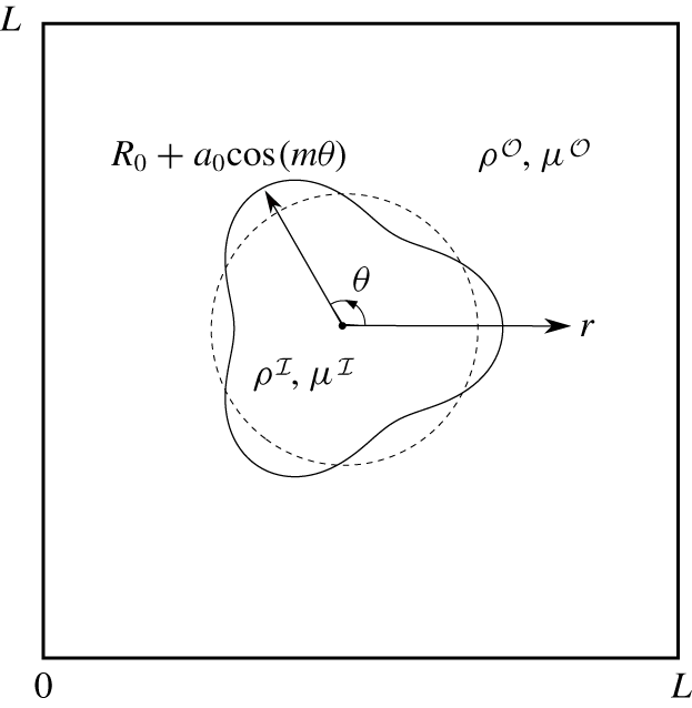
DNS geometry (not to scale).

In this section, we discuss the implementation of an in-house code used for DNS. The in-house code solves for the velocity and pressure fields in two immiscible fluid phases keeping track of the interface between these as a function of time. The basic inviscid algorithm is described in Singh, Farsoiya & Dasgupta (Reference Singh, Farsoiya and Dasgupta2019) and we provide an outline of the salient features here. The incompressible Navier–Stokes equations are written in the following semi-conservative form (Tryggvason, Scardovelli & Zaleski Reference Tryggvason, Scardovelli and Zaleski2011) including surface tension as a body force (Brackbill, Kothe & Zemach Reference Brackbill, Kothe and Zemach1992),
 $$\begin{eqnarray}\displaystyle \unicode[STIX]{x1D735}\boldsymbol{\cdot }\boldsymbol{u}=0,\quad \frac{\unicode[STIX]{x2202}\boldsymbol{u}}{\unicode[STIX]{x2202}t}+\unicode[STIX]{x1D735}\boldsymbol{\cdot }(\boldsymbol{u}\boldsymbol{u})=-\frac{1}{\unicode[STIX]{x1D70C}}\unicode[STIX]{x1D735}p+\frac{1}{\unicode[STIX]{x1D70C}}\unicode[STIX]{x1D735}\boldsymbol{\cdot }[\unicode[STIX]{x1D707}(\unicode[STIX]{x1D735}\boldsymbol{u}+\unicode[STIX]{x1D735}\boldsymbol{u}^{\text{T}})]+\frac{T}{\unicode[STIX]{x1D70C}}\unicode[STIX]{x1D705}\unicode[STIX]{x1D6FF}_{s}\boldsymbol{n}. & & \displaystyle\end{eqnarray}$$
Here  $T$ is the coefficient of surface tension,
 $\unicode[STIX]{x1D70C}$ is the density,
 $\unicode[STIX]{x1D705}$ is the local interfacial curvature,
 $\unicode[STIX]{x1D6FF}_{s}$ is a surface delta function and
 $\boldsymbol{n}$ is the unit normal to the interface. Our code implements the one-fluid approach (Tryggvason et al. Reference Tryggvason, Scardovelli and Zaleski2011) where a single set of (5.1) are solved in both fluid phases (see DNS geometry in figure 6) with density and viscosity being spatially varying functions obtained from a linear weighted combination of the inner and outer fluid density (
 $\unicode[STIX]{x1D70C}^{{\mathcal{I}}},\unicode[STIX]{x1D70C}^{{\mathcal{O}}}$) and viscosity (
 $\unicode[STIX]{x1D707}^{{\mathcal{I}}},\unicode[STIX]{x1D707}^{{\mathcal{O}}}$), based on a colour function. We use the finite-volume approach for which we define an averaged velocity in a control volume (computational cell) as,
 $$\begin{eqnarray}\displaystyle \bar{\boldsymbol{u}}_{i,j}(t)\equiv \frac{1}{V_{i,j}}\int _{V_{i,j}}\boldsymbol{u}(\boldsymbol{x},t)\,\text{d}V, & & \displaystyle\end{eqnarray}$$
where  $V_{i,j}$ denotes the volume (area in two dimensions) of the
 $(i,j)$ computational cell (
 $i,j=1,2,\ldots N$ with
 $N$ being the number of grid points in every spatial direction). We employ a staggered grid and using definition (5.2), we integrate (5.1) (Tryggvason et al. Reference Tryggvason, Scardovelli and Zaleski2011) over a computational control volume (see Tryggvason et al. (Reference Tryggvason, Scardovelli and Zaleski2011) and Singh et al. (Reference Singh, Farsoiya and Dasgupta2019) for details) to obtain
 $$\begin{eqnarray}\displaystyle \frac{\text{d}\bar{\boldsymbol{u}}_{i,j}}{\text{d}t}=\boldsymbol{P}_{i,j}+\boldsymbol{A}_{i,j}+\boldsymbol{D}_{i,j}+\boldsymbol{S}_{i,j},\quad \unicode[STIX]{x1D735}\boldsymbol{\cdot }\bar{\boldsymbol{u}}_{i,j}=0, & & \displaystyle\end{eqnarray}$$
where  $\boldsymbol{P},\boldsymbol{A},\boldsymbol{D}$ and
 $\boldsymbol{S}$ stand for discrete versions of pressure, advection, diffusion and source terms, respectively, (Tryggvason et al. Reference Tryggvason, Scardovelli and Zaleski2011; Singh et al. Reference Singh, Farsoiya and Dasgupta2019). The advection term
 $\boldsymbol{A}_{i,j}$ requires interpolating velocities at the computational cell walls and this is done using a fifth-order weighted essentially non-oscillatory (known as WENO) scheme (Shu Reference Shu2009). The diffusion terms are discretised using a Crank–Nicholson scheme (Patankar Reference Patankar1980). Using Chorin’s projection method (Chorin Reference Chorin1968) the velocity and pressure fields at the
 $(k+1)$th time step (
 $\bar{\boldsymbol{u}}^{k+1},p^{k+1}$) are calculated from the velocity-field at the
 $k$th time step and the incompressibility constraint, using an intermediate velocity field
 $\bar{\boldsymbol{u}}^{\ast }$. Implicit equations for pressure and velocity are iteratively solved using a multigrid Gauss–Siedel V-cycle algorithm (Moin Reference Moin2010). Interface tracking is based on the volume-of-fluid (VOF) method (Hirt & Nichols Reference Hirt and Nichols1981) for which a colour is defined as (Malan et al. Reference Malan, Ling, Scardovelli, Llor and Zaleski2019),
 $$\begin{eqnarray}\displaystyle c_{i,j}(t)\equiv \frac{1}{V}\int _{V}\unicode[STIX]{x1D712}(\boldsymbol{x},t)\,\text{d}V, & & \displaystyle\end{eqnarray}$$
where  $\unicode[STIX]{x1D712}(\boldsymbol{x},t)$ is like a Heaviside function whose value is unity when
 $\boldsymbol{x}$ lies in one of the fluids and zero when it lies in the other. The integration in (5.4) is over a computational control volume. Computational cells fully filled with the inner fluid (density
 $\unicode[STIX]{x1D70C}^{{\mathcal{I}}}$) have
 $c=1$ while those fully filled with the outer fluid (density
 $\unicode[STIX]{x1D70C}^{{\mathcal{O}}}$) have
 $c=0$. Those cells with
 $0\leqslant c\leqslant 1$ have the interface. The density and viscosity field are obtained using
 $\unicode[STIX]{x1D70C}_{i,j}(t)=c_{i,j}(t)\unicode[STIX]{x1D70C}^{{\mathcal{I}}}+(1-c_{i,j}(t))\unicode[STIX]{x1D70C}^{{\mathcal{O}}}$ and
 $\unicode[STIX]{x1D707}_{i,j}(t)=c_{i,j}(t)\unicode[STIX]{x1D707}^{{\mathcal{I}}}+(1-c_{i,j}(t))\unicode[STIX]{x1D707}^{{\mathcal{O}}}$, respectively. Using the
 $c_{i,j}$ field at any given instant of time, the interface is reconstructed using the piecewise, linear, interface reconstruction algorithm (known as LVIRA) (Puckett et al. Reference Puckett, Almgren, Bell, Marcus and Rider1997). Note that in DNS data, contours of constant
 $c_{ij}$ (between zero and unity) are approximately analogous to
 $F$ in (2.7) since by definition, the interface is a curve on which
 $F=0$. In order to evolve
 $c_{i,j}$ in time, the discrete form of an advection equation (Malan et al. Reference Malan, Ling, Scardovelli, Llor and Zaleski2019; Singh et al. Reference Singh, Farsoiya and Dasgupta2019) is obtained by integrating over a computational control volume. An important feature of the VOF algorithm is that fluxes through the control volume boundaries are estimated geometrically. We use the forward and reverse algebraic relations described in Scardovelli & Zaleski (Reference Scardovelli and Zaleski2000) for calculating these fluxes.
In flows dominated by capillary effects as studied here, accurate curvature calculation is crucial. We use the direction-averaged curvature (DAC) method used earlier in Lörstad & Fuchs (Reference Lörstad and Fuchs2004) and Kalland (Reference Kalland2008) for curvature estimation. Details of the DAC algorithm are described in figure 1 of Singh et al. (Reference Singh, Farsoiya and Dasgupta2019). The time stepping used in the code is based on a combination of Courant–Friedrichs–Lewy (CFL) based restrictions as well as the minimum step size based on a capillary time scale constraint i.e.  $\unicode[STIX]{x0394}t=\text{CFL}\times [\min (\frac{1}{2}(\unicode[STIX]{x1D6E5}/U_{max}),\sqrt{(\unicode[STIX]{x1D70C}^{{\mathcal{I}}}+\unicode[STIX]{x1D70C}^{{\mathcal{O}}})\unicode[STIX]{x1D6E5}^{3}/4\unicode[STIX]{x03C0}T})]$, where
 $\unicode[STIX]{x1D6E5}$ is the uniform mesh size and we have used a
 $\text{CFL}=0.25$. Note that as our numerical formulation for discretising the viscous terms in (5.3) is implicit, there is no restriction on
 $\unicode[STIX]{x0394}t$ due to viscosity. Many additional test cases (including comparisons with experimental data) have been performed for benchmarking the in-house solver. Results from these are provided in § 4 of the accompanying supplementary material.
6 Results and discussion
The DNS geometry is shown in figure 6. The simulation domain size  $L$ was chosen to be sufficiently large relative to the undisturbed filament radius
 $R_{0}$, to effectively mimic a radially unbounded domain. For the present purpose, we found that choosing
 $L/R=10$ was sufficient to eliminate finite domain effects on the time scale of our simulations. The normal velocity on all computational domain boundaries is zero. We also impose zero normal derivative for the tangential component of velocity, pressure and volume fraction. The DNS are governed by five non-dimensional parameters viz.
 $m$, Laplace number
 $La$, density ratio
 $\unicode[STIX]{x1D70C}_{r}=\unicode[STIX]{x1D70C}^{{\mathcal{I}}}/\unicode[STIX]{x1D70C}^{{\mathcal{O}}}$, viscosity ratio
 $\unicode[STIX]{x1D707}_{r}\equiv \unicode[STIX]{x1D707}^{{\mathcal{I}}}/\unicode[STIX]{x1D707}^{{\mathcal{O}}}$ and
 $\unicode[STIX]{x1D716}\equiv a_{0}m/R_{0}$, a nonlinearity parameter. In order to compare results obtained from DNS with the linearised theory presented earlier, we require the nonlinearity parameter
 $\unicode[STIX]{x1D716}\ll 1$. In addition we need to ensure that the density and viscosity ratio are small i.e.
 $\unicode[STIX]{x1D70C}_{r},\;\unicode[STIX]{x1D707}_{r}\ll 1$, in order to keep dynamic effects of the fluid inside the filament to a minimum. All DNS parameters are summarised in table 2. All viscous simulations have been performed choosing density ratio
 $\unicode[STIX]{x1D70C}_{r}$ ranging from
 $10^{-4}-1$ and viscosity ratio in the range
 $\unicode[STIX]{x1D707}_{r}\approx 10^{-3}$ and
 $10^{-4}$. For minimising nonlinear effects, we chose
 $\unicode[STIX]{x1D716}=0.1$ in most simulations. Note that in table 2, the values for viscosity of the outer fluid (
 $\unicode[STIX]{x1D707}^{{\mathcal{O}}}$) were chosen to ensure integral values of
 $La$. All simulations are initiated with an interfacial perturbation of the form
 $r=R_{0}+a_{0}\cos (m\unicode[STIX]{x1D703})$ with zero velocity everywhere in the domain. The resultant motion of the interface is tracked in time and the vorticity field is computed from the velocity field obtained in DNS. As a first step, we have validated the inviscid dispersion relation (1.2) by imposing an azimuthal Fourier mode
 $m=2$ in our solver and integrating the inviscid equations of motion (parameters corresponding to case
 $0$ in table 2). It is shown in figure 4(a) of the supplementary material that the time signal obtained from DNS and fitted to
 $a(t)/a_{0}=\cos (\unicode[STIX]{x1D714}_{0}t)$ shows good agreement (see Singh et al. (Reference Singh, Farsoiya and Dasgupta2019) for more numerical tests on this inviscid problem). For figures 7(a), 7(b), 8(a) and 8(b), all time signals are obtained by tracking the interface at
 $\unicode[STIX]{x1D703}=0$ (see figure 6), although choosing any other
 $\unicode[STIX]{x1D703}$ would lead to identical signals. We compare data obtained from DNS with predictions from expressions (4.23) and (4.25). Note that for evaluating the discrete part of both expressions (i.e. the summed over terms on the right-hand side), we have employed the Mathematica function FindRoot (Wolfram Research, Inc. 2016). The integrals in both expressions are solved numerically using the Mathematica function NIntegrate (Wolfram Research, Inc. 2016). The script files for doing this are provided as additional supplementary material.
For NMA (a)  $C=0.5+0.57\text{i}$ and (b)
 $C=0.5+0.166\text{i}$. (a) Case 1 in table 2, (b) case
 $2$.

For NMA (a)  $C=0.5+0.66\text{i}$ and (b)
 $C=0.5+0.169\text{i}$. (a) Case
 $3$, (b) case
 $4$.

Effect of change of (a)  $\unicode[STIX]{x1D716}$, (b)
 $\unicode[STIX]{x1D70C}_{r}$. (a) Cases 5, 6 and 7. (b) Cases 8, 9 and 10.

Comparing figures 7(a) and 7(b), it is seen that the solution to the IVP given by (4.23) agrees very well with DNS. In contrast, the discrete part of expression (4.23) (labelled as DS) shows a poor agreement at  $t=0$ especially at large values of viscosity (smaller
 $La$). The same behaviour is also observed in figures 8(a) and 8(b) for a Fourier mode with
 $m=3$. We also compare with an approximation labelled as the normal mode approximation (NMA) in figures 7(a)–8(b). This approximation utilises the observation that the discrete spectrum has two roots,
 $\unicode[STIX]{x1D70E}$ and
 $\bar{\unicode[STIX]{x1D70E}}$, only. Consequently it is possible to obtain an approximate solution for the amplitude
 $a(t)=C\exp (\unicode[STIX]{x1D70E}t)+\bar{C}\exp (\bar{\unicode[STIX]{x1D70E}}t)$ with
 $C$ being a complex constant whose real and imaginary parts are determined by initial conditions
 $a(0)=a_{0}$ and
 ${\dot{a}}(0)=0$ (see Farsoiya et al. Reference Farsoiya, Mayya and Dasgupta2017). Unlike the DS approximation, the NMA has the advantage that by construction it satisfies initial conditions for
 $a(t)$. It is seen in figures 7(a)–8(b) that while the NMA is a better approximation at early times, the DS approximation improves over it at later stages showing less disagreement with DNS, even at lower values of
 $La$. We also observe that for
 $La=2.5$, the interface continues to show underdamped behaviour (see figures 7a and 8a), consistent with our predictions from the dispersion relation (3.23) in § 3.1. Figures 9(a) and 9(b) show the effect of increasing the nonlinearity parameter
 $\unicode[STIX]{x1D716}$ and density ratio
 $\unicode[STIX]{x1D70C}_{r}$. Note that with we have used a relatively high value of Laplace number purposely in order to reduce damping and highlight nonlinear effects. It is seen from figure 9(a) that nonlinear effects are quite pronounced at
 $\unicode[STIX]{x1D716}=0.5$. Similarly, systematic effects of inertia of the gas inside is seen in figure 9(b) as
 $\unicode[STIX]{x1D70C}_{r}$ is increased, with large deviations from the present theoretical predictions seen at
 $\unicode[STIX]{x1D70C}_{r}=1$.
For comparing vorticity fields, we note that our in-house solver is written in Cartesian coordinates ( $x$–
 $y$) while the analytical expressions for
 $\hat{\unicode[STIX]{x1D6FA}}(r,t)$ (4.25) are obtained in plane-polar (
 $r$–
 $\unicode[STIX]{x1D703}$) coordinates (see figure 1a). It is shown in the supplementary material, § 5 that the out-of-plane
 $z$ component of the vorticity
 $\unicode[STIX]{x1D714}_{z}^{Cartesian}\equiv (\unicode[STIX]{x2202}v/\unicode[STIX]{x2202}x)-(\unicode[STIX]{x2202}u/\unicode[STIX]{x2202}y)$, is the same as the (axial)
 $z$ component of vorticity in cylindrical coordinates (or polar coordinates) (
 $\unicode[STIX]{x1D714}\equiv (1/r)\{\unicode[STIX]{x2202}/\unicode[STIX]{x2202}r(ru_{\unicode[STIX]{x1D703}})-(\unicode[STIX]{x2202}u_{r}/\unicode[STIX]{x2202}\unicode[STIX]{x1D703})\}$). In figures 10(a) and 10(b) we show the contour of the vorticity field
 $\unicode[STIX]{x1D714}(r,\unicode[STIX]{x1D703},t)$ obtained from DNS at
 $t=\unicode[STIX]{x03C0}/\unicode[STIX]{x1D714}_{0}$. In both figures, the vorticity field inside the filament (i.e.
 $0\leqslant r\leqslant R_{0}+\unicode[STIX]{x1D702}$) has been removed to enable comparison with the analytical prediction from IVP in figures 11(a) and 11(b). The four lobes seen in these figures correspond to an azimuthal dependence of
 $\sin (2\unicode[STIX]{x1D703})$. Note that the sign is opposite as
 $\unicode[STIX]{x1D6FA}(r,t)$ is negative at the instant of time. Figure 10(a) corresponds to a higher viscosity and thus has a thicker vorticity layer compared to figure 10(b). For comparison, we have also plotted the analytical prediction from (4.2) and (4.25) in figures 11(a) and 11(b). A good agreement is observed in the analytically predicted vorticity field vis-à-vis DNS data. The difference between analytical and DNS vorticity data in figures 10(a), 10(b) and 11(a), 11(b) are plotted as contours in figures 12(a) and 12(b). It is seen that apart from thin regions very close to the interface, a very good agreement is found. The reasons for this deviation close to the interface are discussed below.
DNS vorticity contours for  $\unicode[STIX]{x1D714}$; (a)
 $t=\unicode[STIX]{x03C0}/\unicode[STIX]{x1D714}_{0}$, case
 $1$, (b)
 $t=\unicode[STIX]{x03C0}/\unicode[STIX]{x1D714}_{0}$, case
 $2$.

Analytical vorticity contours; (a)  $t=\unicode[STIX]{x03C0}/\unicode[STIX]{x1D714}_{0}$, case
 $1$, (b)
 $t=\unicode[STIX]{x03C0}/\unicode[STIX]{x1D714}_{0}$, case
 $2$.

Difference between analytical and DNS contours for vorticity; (a)  $t=\unicode[STIX]{x03C0}/\unicode[STIX]{x1D714}_{0}$, case
 $1$, (b)
 $t=\unicode[STIX]{x03C0}/\unicode[STIX]{x1D714}_{0}$, case
 $2$.

Cancellation of vorticity at  $t=0$ between CS and DS modes.

For further quantitative comparison, figures 13 and 14(a–d) show the vorticity profiles outside the filament ( $r\geqslant R_{0}+\unicode[STIX]{x1D702}$) at
 $\unicode[STIX]{x1D703}=\unicode[STIX]{x03C0}/4$ as a function of radius, at different instants of time. The parameters correspond to case
 $1$ in table 2. A good match is seen in every case. The slight disagreement seen between DNS and analytical prediction (4.25) near the interface
 $r=R_{0}+\unicode[STIX]{x1D702}\approx 1$, is to be expected as the interface in DNS experiences a small amount of tangential stress exerted by the fluid inside the filament. This is not taken into account in the theory where the interface is treated as being free of tangential stress at all times (see boundary condition (2.9)). Note that independent of whether the motion in the gas phase inside the filament is modelled or not, tangential stress at the interface is continuous. A comparison of prediction from (4.25) and CS and DS contributions at
 $t=0$ are shown in figure 13. As we solve for zero initial vorticity, the CS and DS contributions are exactly equal and opposite at
 $t=0$ at all radii. The temporal evolution of the vorticity field with radius, are shown in figure 14(a–d). It is seen that the DS approximation to the vorticity field given by the summation terms alone in (4.25), follows the same qualitative trend as DNS but has a large quantitative mismatch. In contrast the sum of CS and DS provides very good agreement at all times. Note from these figures that at large radii, wherever the DS contribution is slightly different from zero, the CS is also different from zero and of the same order of magnitude, although it has the opposite sign. The DNS signal which contains contributions from the CS and the DS together, as implied by (4.25), receives an almost equal and opposite contribution from both, especially at large radii thus adding up to near zero there.
 $\hat{\unicode[STIX]{x1D6FA}}$ versus radius at
 $\unicode[STIX]{x1D703}=\unicode[STIX]{x03C0}/4$ at different times: case
 $1$ in table 2. (a)
 $t=\unicode[STIX]{x03C0}/2\unicode[STIX]{x1D714}_{0}$, case
 $1$, (b)
 $t=\unicode[STIX]{x03C0}/\unicode[STIX]{x1D714}_{0}$, case
 $1$, (c)
 $t=3\unicode[STIX]{x03C0}/2\unicode[STIX]{x1D714}_{0}$, case
 $1$, (d)
 $t=2\unicode[STIX]{x03C0}/\unicode[STIX]{x1D714}_{0}$, case
 $1$.

7 Conclusions
In this study, we have analysed the temporal spectrum of linearised, azimuthal Fourier modes on a hollow cylindrical filament, surrounded by radially unbounded, quiescent, viscous fluid. The base state is found to be stable to all azimuthal Fourier modes of standing wave form. Using normal mode analysis, we obtain the dispersion relation governing the discrete spectrum for the problem. The dispersion relation is a transcendental equation whose numerical (and perturbative) solution predicts that all azimuthal Fourier modes respond in an underdamped manner, even at large values of fluid viscosity. Using normal modes, we also show that in addition to the discrete spectrum, the problem admits a continuous spectrum. The discrete spectrum eigenfunctions decay exponentially at large radii and thus cannot adequately represent far field perturbations. A continuum of uncountably infinite eigenfunctions are also found which decay to zero algebraically at large radii and are essential for representing far field perturbations. The completeness theorem for the perturbation vorticity field is a sum over the discrete eigenmodes and an integral over the continuous ones. A similar completeness theorem is also obtained for the amplitude of the standing wave. We solve the linearised IVP for a perturbation taken to be an azimuthal Fourier mode with zero perturbation vorticity. Analytical expressions governing the time dependence of the amplitude of the standing wave and its associated vorticity field are obtained in the Laplace  $s$ domain. Analysis of these show that in addition to poles, they also have branch points on the complex
 $s$ plane. Laplace inversion of these expressions using the Cauchy residue theorem shows that the discrete spectrum comes from the residue at the zeroes (which manifest themselves as poles) of the dispersion relation while the continuous spectrum comes from the difference in contribution on either side of the branch cut. The zero vorticity initial condition investigated here has projections on the discrete as well as the continuous spectrum. Consequently the discrete as well as the continuum eigenmodes are excited initially and the subsequent motion of the interface resembles a standing wave whose amplitude is a sum of discrete exponentials and an integral over a continuous range of exponentials. Linearised analytical predictions are compared to DNS conducted using a code developed in-house and excellent agreement is observed with the IVP solution at all times for small values of the nonlinearity parameter
 $\unicode[STIX]{x1D716}$. In contrast, the discrete spectrum approximation is found to be a poor approximation at early times, especially at
 $O(1)$ Laplace numbers. Future lines of analysis involve taking into account a non-zero vorticity perturbation
 $\unicode[STIX]{x1D6FA}(r,0)$ in the far field for a three-dimensional hollow filament. This is currently underway and will be reported subsequently.
Supplementary materials
Supplementary materials are available at https://doi.org/10.1017/jfm.2019.809.
Acknowledgements
R.D. thanks R. Govindarajan for an invitation to the ICTS turbulence meeting (https://www.icts.res.in/discussion-meeting/taly2018) where some ideas contained here were presented. We thank A. Sharma and K. M. Kalland for implementation of the WENO and DAC algorithm. R.D. and P.K.F. acknowledge financial support from Industrial Research and Consultancy Centre (IRCC), IIT Bombay (no. 14IRCCSG007) and Science and Engineering Research Board (SERB, Dept. Science and Technology (DST), Govt. of India (no. EMR/2016/000830) for a cluster. A.R. acknowledges financial support from SERB-DST (no. ECR/2017/001940) and IIT Madras initiation grant APM1617836NFIGANUB.
Appendix A
A consistency check on (3.23) is to demonstrate that it reduces to the viscous dispersion relation in Cartesian geometry (see Lamb Reference Lamb1993) in the limit  $m\rightarrow \infty ,R_{0}\rightarrow \infty$ such that
 $m/R_{0}\rightarrow k$ where
 $k$ is the wavenumber in Cartesian
 $(x,z)$ coordinates (i.e.
 $\unicode[STIX]{x1D702}(x,t)=a_{0}\cos (kx)$). The following asymptotic formulae (as
 $\unicode[STIX]{x1D708}\rightarrow \infty$) (Abramowitz & Stegun Reference Abramowitz and Stegun1965) are necessary for further analysis:
 $$\begin{eqnarray}\displaystyle & \displaystyle \text{K}_{\unicode[STIX]{x1D708}}(\unicode[STIX]{x1D708}z)\sim \left(\frac{\unicode[STIX]{x03C0}}{2\unicode[STIX]{x1D708}}\right)^{1/2}\frac{\exp \left[-\unicode[STIX]{x1D708}\unicode[STIX]{x1D702}\right]}{(1+z^{2})^{1/4}}, & \displaystyle\end{eqnarray}$$
 $$\begin{eqnarray}\displaystyle & \displaystyle \text{K}_{\unicode[STIX]{x1D708}}^{\prime }(\unicode[STIX]{x1D708}z)\sim -\left(\frac{\unicode[STIX]{x03C0}}{2\unicode[STIX]{x1D708}}\right)^{1/2}\frac{(1+z^{2})^{1/4}}{z}\exp \left[-\unicode[STIX]{x1D708}\unicode[STIX]{x1D702}\right], & \displaystyle\end{eqnarray}$$
with  $\unicode[STIX]{x1D702}\equiv (1+z^{2})^{1/2}+\ln [z/(1+(1+z^{2})^{1/2})]$. Consider the limit
 $m\rightarrow \infty ,R_{0}\rightarrow \infty$ with
 $m/R_{0}=k$. Defining
 $\hat{k}\equiv k\sqrt{\unicode[STIX]{x1D708}/\unicode[STIX]{x1D70E}}$ and using (A 1), (A 2) we obtain the following asymptotic expressions:
 $$\begin{eqnarray}\displaystyle & \displaystyle \frac{\text{K}_{m-1}(\hat{R}_{0})}{\text{K}_{m-1}^{\prime }(\hat{R}_{0})}\sim -{\displaystyle \frac{1}{(\hat{k}^{2}+1)^{1/2}}}, & \displaystyle\end{eqnarray}$$
 $$\begin{eqnarray}\displaystyle & \displaystyle \frac{\text{K}_{m+1}(\hat{R}_{0})}{\text{K}_{m-1}^{\prime }(\hat{R}_{0})}\sim -\left(\frac{m-1}{m+1}\right)^{1/2}\exp [-\{(m+1)\unicode[STIX]{x1D702}_{2}-(m-1)\unicode[STIX]{x1D702}_{1}\}]\frac{z_{1}}{\{(1+z_{1}^{2})(1+z_{2}^{2})\}^{1/4}}. & \displaystyle \nonumber\\ \displaystyle & & \displaystyle\end{eqnarray}$$
Here
 $$\begin{eqnarray}\unicode[STIX]{x1D702}_{2,1}=(1+z_{2,1}^{2})^{1/2}+\ln \left[{\displaystyle \frac{z_{2,1}}{1+\left(1+z_{2,1}^{2}\right)^{1/2}}}\right]\quad \text{and}\quad z_{2,1}\equiv {\displaystyle \frac{\hat{R}_{0}}{m\pm 1}}={\displaystyle \frac{1}{\hat{k}}}\left(1\mp {\displaystyle \frac{1}{m}}\right).\end{eqnarray}$$
Asymptotic expressions for  $\unicode[STIX]{x1D702}_{2,1}$ may be obtained as follows:
 $$\begin{eqnarray}\displaystyle \unicode[STIX]{x1D702}_{2,1} & {\sim} & \displaystyle \left[1+{\displaystyle \frac{1}{\hat{k}^{2}}}\left(1\mp {\displaystyle \frac{2}{m}}\right)\right]^{1/2}+\ln \left[{\displaystyle \frac{{\displaystyle \frac{1}{\hat{k}}}\left(1\pm {\displaystyle \frac{1}{m}}\right)}{1+\left\{1+{\displaystyle \frac{1}{\hat{k}^{2}}}\left(1\mp {\displaystyle \frac{2}{m}}\right)\right\}^{1/2}}}\right]\nonumber\\ \displaystyle & {\sim} & \displaystyle \left(1+{\displaystyle \frac{1}{\hat{k}^{2}}}\right)^{1/2}\left(1\mp \frac{1}{m(\hat{k}^{2}+1)}\right)+\ln \left[{\displaystyle \frac{1\mp {\displaystyle \frac{1}{m}}}{\hat{k}+(\hat{k}^{2}+1)^{1/2}\left\{1\mp {\displaystyle \frac{1}{m(\hat{k}^{2}+1)}}\right\}}}\right].\nonumber\\ \displaystyle & & \displaystyle\end{eqnarray}$$
Using the Taylor expansion of  $\ln (1+\unicode[STIX]{x1D716})$ for
 $\unicode[STIX]{x1D716}\ll 1$, we obtain from (A 6)
 $$\begin{eqnarray}\displaystyle \unicode[STIX]{x1D702}_{2,1} & {\sim} & \displaystyle {\displaystyle \frac{(\hat{k}^{2}+1)^{1/2}}{\hat{k}}}\mp {\displaystyle \frac{1}{m\hat{k}(\hat{k}^{2}+1)^{1/2}}}\mp \frac{1}{m}-\ln \left[\hat{k}+(\hat{k}^{2}+1)^{1/2}\right]\nonumber\\ \displaystyle & \pm & \displaystyle {\displaystyle \frac{1}{m(\hat{k}^{2}+1)^{1/2}\{\hat{k}+(\hat{k}^{2}+1)^{1/2}\}}}\nonumber\\ \displaystyle & {\sim} & \displaystyle {\displaystyle \frac{(\hat{k}^{2}+1)^{1/2}}{\hat{k}}}-\ln \left[\hat{k}+(\hat{k}^{2}+1)^{1/2}\right]\mp {\displaystyle \frac{(\hat{k}^{2}+1)^{1/2}}{m\hat{k}}}.\end{eqnarray}$$
Using (A 7), we obtain at leading order,
 $$\begin{eqnarray}\displaystyle \exp [-\{(m+1)\unicode[STIX]{x1D702}_{2}-(m-1)\unicode[STIX]{x1D702}_{1}\}]\sim 1+2\hat{k}^{2}+2\hat{k}(\hat{k}^{2}+1)^{1/2}. & & \displaystyle\end{eqnarray}$$
Equations (A 3), (A 4) and (A 8) imply the following leading-order behaviour:
 $$\begin{eqnarray}\displaystyle \frac{\text{K}_{m+1}(\hat{R}_{0})}{\text{K}_{m-1}^{\prime }(\hat{R}_{0})}\sim -{\displaystyle \frac{1+2\hat{k}^{2}+2\hat{k}(\hat{k}^{2}+1)^{1/2}}{(\hat{k}^{2}+1)^{1/2}}},\quad {\displaystyle \frac{{\mathcal{G}}(\hat{R}_{0})}{\hat{R}_{0}\text{K}_{m-1}^{\prime }(\hat{R}_{0})}}\sim -\frac{1+2\hat{k}(\hat{k}^{2}+1)^{1/2}}{2\hat{k}(\hat{k}^{2}+1)^{1/2}}. & & \displaystyle \nonumber\\ \displaystyle & & \displaystyle\end{eqnarray}$$
Re-writing the dispersion relation (3.23) for a hollow jet, in terms of the frequency  $\unicode[STIX]{x1D70E}$ and using the asymptotic expressions (A 9), we obtain
 $$\begin{eqnarray}\displaystyle \unicode[STIX]{x1D70E}^{2}+\unicode[STIX]{x1D708}k^{2}\left[\frac{1+4\hat{k}(\hat{k}^{2}+1)^{1/2}}{\hat{k}(\hat{k}^{2}+1)^{1/2}}\right]\unicode[STIX]{x1D70E}+\frac{Tk^{3}}{\unicode[STIX]{x1D70C}}\left[\frac{(\hat{k}^{2}+1)^{1/2}+\hat{k}}{(\hat{k}^{2}+1)^{1/2}}\right]=0. & & \displaystyle\end{eqnarray}$$
Equation (A 10) may be further written as
 $$\begin{eqnarray}\displaystyle & & \displaystyle \unicode[STIX]{x1D70E}^{2}[(\hat{k}^{2}+1)^{1/2}\{(\hat{k}^{2}+1)^{1/2}-\hat{k}\}]+\unicode[STIX]{x1D708}k^{2}\left[\frac{1}{\hat{k}}\{(\hat{k}^{2}+1)^{1/2}-\hat{k}\}\{1+4\hat{k}(\hat{k}^{2}+1)^{1/2}\}\right]\unicode[STIX]{x1D70E}\nonumber\\ \displaystyle & & \displaystyle \qquad +\,\frac{Tk^{3}}{\unicode[STIX]{x1D70C}}=0.\end{eqnarray}$$
Using  $\hat{k}=k(\unicode[STIX]{x1D708}/\unicode[STIX]{x1D70E})^{1/2}$, we obtain from (A 11)
 $$\begin{eqnarray}\displaystyle & & \displaystyle \unicode[STIX]{x1D70E}^{2}\left[\left(k^{2}\frac{\unicode[STIX]{x1D708}}{\unicode[STIX]{x1D70E}}+1\right)^{1/2}\left\{\left(k^{2}\frac{\unicode[STIX]{x1D708}}{\unicode[STIX]{x1D70E}}+1\right)^{1/2}-k\left(\frac{\unicode[STIX]{x1D708}}{\unicode[STIX]{x1D70E}}\right)^{1/2}\right\}\right]\nonumber\\ \displaystyle & & \displaystyle +\,\unicode[STIX]{x1D708}k^{2}\left[\frac{1}{k\left({\displaystyle \frac{\unicode[STIX]{x1D708}}{\unicode[STIX]{x1D70E}}}\right)^{1/2}}\left\{\left(k^{2}\frac{\unicode[STIX]{x1D708}}{\unicode[STIX]{x1D70E}}+1\right)^{1/2}-k\left(\frac{\unicode[STIX]{x1D708}}{\unicode[STIX]{x1D70E}}\right)^{1/2}\right\}\left\{1+4k\left(\frac{\unicode[STIX]{x1D708}}{\unicode[STIX]{x1D70E}}\right)^{1/2}\left(k^{2}\frac{\unicode[STIX]{x1D708}}{\unicode[STIX]{x1D70E}}+1\right)^{1/2}\right\}\right]\unicode[STIX]{x1D70E}\nonumber\\ \displaystyle & & \displaystyle +\,\frac{Tk^{3}}{\unicode[STIX]{x1D70C}}=0.\end{eqnarray}$$
Equation (A 12) may be written as,
 $$\begin{eqnarray}\displaystyle & & \displaystyle \unicode[STIX]{x1D70E}^{2}\left[k^{2}\frac{\unicode[STIX]{x1D708}}{\unicode[STIX]{x1D70E}}+1-k\sqrt{\frac{\unicode[STIX]{x1D708}}{\unicode[STIX]{x1D70E}}}\left(k^{2}\frac{\unicode[STIX]{x1D708}}{\unicode[STIX]{x1D70E}}+1\right)^{1/2}\right]+\unicode[STIX]{x1D708}k^{2}\left[\left(\frac{\unicode[STIX]{x1D708}k^{2}+\unicode[STIX]{x1D70E}}{\unicode[STIX]{x1D708}k^{2}}\right)^{1/2}\right.\nonumber\\ \displaystyle & & \displaystyle \qquad \left.+\,\frac{4k^{2}\unicode[STIX]{x1D708}}{\unicode[STIX]{x1D70E}}+4-1-4k\left(\frac{\unicode[STIX]{x1D708}}{\unicode[STIX]{x1D70E}}\right)^{1/2}\left(\frac{\unicode[STIX]{x1D708}k^{2}+\unicode[STIX]{x1D70E}}{\unicode[STIX]{x1D70E}}\right)^{1/2}\right]\unicode[STIX]{x1D70E}+\frac{Tk^{3}}{\unicode[STIX]{x1D70C}}=0.\end{eqnarray}$$
After cancellations (A 13) simplifies to
 $$\begin{eqnarray}\displaystyle \left(\unicode[STIX]{x1D70E}+2\unicode[STIX]{x1D708}k^{2}\right)^{2}+\frac{Tk^{3}}{\unicode[STIX]{x1D70C}}=4\unicode[STIX]{x1D708}^{2}k^{3}\left(\frac{\unicode[STIX]{x1D708}k^{2}+\unicode[STIX]{x1D70E}}{\unicode[STIX]{x1D708}}\right)^{1/2}, & & \displaystyle\end{eqnarray}$$
which is the dispersion relation provided in Lamb (Reference Lamb1993).
Appendix B
We show here that the dispersion relation (3.23) has the correct inviscid limit (1.2) and for small viscosity yields a correction to this. Re-writing (3.23) in dimensional variables we obtain
 $$\begin{eqnarray}\displaystyle & & \displaystyle R_{0}^{4}\frac{\unicode[STIX]{x1D70E}^{2}}{\unicode[STIX]{x1D708}^{2}}+\left\{2m(m+1)\left(1-\frac{{\displaystyle \frac{\hat{R}_{0}^{2}}{2m}}\text{K}_{m+1}(\hat{R}_{0})-(m-1)\text{K}_{m-1}(\hat{R}_{0})}{\hat{R}_{0}\text{K}_{m-1}^{\prime }(\hat{R}_{0})}\right)\right\}R_{0}^{2}\frac{\unicode[STIX]{x1D70E}}{\unicode[STIX]{x1D708}}\nonumber\\ \displaystyle & & \displaystyle \qquad +\,\frac{TR_{0}\unicode[STIX]{x1D70C}}{\unicode[STIX]{x1D707}^{2}}m(m^{2}-1)\left(1-{\displaystyle \frac{(m+1)}{\hat{R}_{0}}}{\displaystyle \frac{\text{K}_{m-1}(\hat{R}_{0})}{\text{K}_{m-1}^{\prime }(\hat{R}_{0})}}\right)=0,\end{eqnarray}$$
which may be written as
 $$\begin{eqnarray}\displaystyle & & \displaystyle \unicode[STIX]{x1D70E}^{2}+\frac{2m(m+1)\unicode[STIX]{x1D708}}{R_{0}^{2}}\left(1-\frac{1}{2m}\frac{\hat{R}_{0}\text{K}_{m+1}(\hat{R}_{0})}{\text{K}_{m-1}^{\prime }(\hat{R}_{0})}+(m-1)\frac{\text{K}_{m-1}(\hat{R}_{0})}{\hat{R}_{0}\text{K}_{m-1}^{\prime }(\hat{R}_{0})}\right)\unicode[STIX]{x1D70E}\nonumber\\ \displaystyle & & \displaystyle \qquad +\,\unicode[STIX]{x1D714}_{0}^{2}\left(1-(m+1){\displaystyle \frac{\text{K}_{m-1}(\hat{R}_{0})}{\hat{R}_{0}\text{K}_{m-1}^{\prime }(\hat{R}_{0})}}\right)=0.\end{eqnarray}$$
Using the leading-order behaviour at large  $z$,
 $$\begin{eqnarray}\text{K}_{m}(z)\sim \left(\frac{\unicode[STIX]{x03C0}}{2z}\right)^{1/2}\exp (-z)\left[1+\frac{a_{1}(m)}{z}+\cdots \,\right]\end{eqnarray}$$
and
 $$\begin{eqnarray}\text{K}_{m}^{\prime }(z)=-\left(\frac{\unicode[STIX]{x03C0}}{2z}\right)^{1/2}\exp (-z)\left[1+\frac{b_{1}(m)}{z}+\cdots \,\right]\end{eqnarray}$$
with  $a_{1}(m)=(4m^{2}-1)/8$ and
 $b_{1}(m)=(4m^{2}+3)/8$ (Abramowitz & Stegun Reference Abramowitz and Stegun1965) and for small viscosity
 $\unicode[STIX]{x1D708}$, posing the expansion
 $$\begin{eqnarray}\displaystyle \unicode[STIX]{x1D70E}=\unicode[STIX]{x1D70E}_{0}+\unicode[STIX]{x1D708}^{1/2}\unicode[STIX]{x1D70E}_{1}+\unicode[STIX]{x1D708}\unicode[STIX]{x1D70E}_{2}+\unicode[STIX]{x1D70E}_{3}\unicode[STIX]{x1D708}^{3/2}+\unicode[STIX]{x1D70E}_{4}\unicode[STIX]{x1D708}^{2}+\cdots & & \displaystyle\end{eqnarray}$$
we obtain at various orders the following coefficients:
 $$\begin{eqnarray}\displaystyle \left.\begin{array}{@{}c@{}}\displaystyle \unicode[STIX]{x1D70E}_{0}=\text{i}\unicode[STIX]{x1D714}_{0},\quad \unicode[STIX]{x1D70E}_{1}=0,\quad \unicode[STIX]{x1D70E}_{2}=-\frac{2m(m+1)}{R_{0}^{2}},\\ \displaystyle \unicode[STIX]{x1D70E}_{3}=\frac{2m\left(1+m\right)^{2}}{R_{0}^{3}\unicode[STIX]{x1D714}_{0}^{1/2}}\exp \left(-\text{i}\unicode[STIX]{x03C0}/4\right),\quad \unicode[STIX]{x1D70E}_{4}=\frac{3\text{i}m(m+1)^{2}}{R_{0}^{4}\unicode[STIX]{x1D714}_{0}}\cdots \,.\end{array}\right\} & & \displaystyle\end{eqnarray}$$
The second series is the complex conjugate of the above.
Appendix C
The expression for  $\tilde{{\mathcal{C}}}(s)$ in (4.9) is obtained using Cramer’s rule on equations (4.12)–(4.14). This is
 $$\begin{eqnarray}\displaystyle \tilde{{\mathcal{C}}}(s) & = & \displaystyle {\displaystyle \frac{\left|\begin{array}{@{}ccc@{}}s & a_{0} & {\displaystyle \frac{m}{R_{0}}}\\ 0 & 0 & {\displaystyle \frac{2m(m+1)}{R_{0}^{2}}}\\ -{\displaystyle \frac{T}{\unicode[STIX]{x1D70C}R_{0}^{2}}}(1-m^{2}) & 0 & -s\left(1+{\displaystyle \frac{2m(m+1)}{h^{2}R_{0}^{2}}}\right)\end{array}\right|}{\left|\begin{array}{@{}ccc@{}}s & -{\displaystyle \frac{\text{K}_{m-1}(hR_{0})}{2h}} & {\displaystyle \frac{m}{R_{0}}}\\ 0 & -\text{K}_{m-1}^{\prime }(hR_{0}) & {\displaystyle \frac{2m(m+1)}{R_{0}^{2}}}\\ -{\displaystyle \frac{T}{\unicode[STIX]{x1D70C}R_{0}^{2}}}(1-m^{2}) & {\displaystyle \frac{\unicode[STIX]{x1D708}}{hR_{0}}}{\mathcal{G}}(hR_{0}) & -s\left(1+{\displaystyle \frac{2m(m+1)}{h^{2}R_{0}^{2}}}\right)\end{array}\right|}}\nonumber\\ \displaystyle & = & \displaystyle \frac{2(m+1)\unicode[STIX]{x1D714}_{0}^{2}}{R_{0}}\left(\frac{a_{0}}{s^{2}+s{\mathcal{M}}(s)+\unicode[STIX]{x1D714}_{0}^{2}\unicode[STIX]{x1D712}(s)}\right)\frac{1}{\text{K}_{m-1}^{\prime }(hR_{0})}.\end{eqnarray}$$
Appendix D
As  $\tilde{a}(s)$ in (4.15) has branch points at
 $s=0$ and
 $s=\infty$, we need to choose a branch of
 $\tilde{a}(s)$ to ensure single-valuedness. Defining
 $-\unicode[STIX]{x03C0}\leqslant \arg (s)\leqslant \unicode[STIX]{x03C0}$, we choose the branch cut to be the negative real axis. Using the Cauchy residue theorem, the Laplace inversion of (4.21) may be obtained using the keyhole contour shown in figure 15.
The poles inside the contour are those roots of  ${\mathcal{Q}}(s)$ which satisfy the constraint
 $\text{Re}(\sqrt{s/\unicode[STIX]{x1D708}})>0$ (i.e. lie on the principal sheet). It has been checked numerically using Mathematica FindRoot (Wolfram Research, Inc. 2016) that
 ${\mathcal{Q}}(s)=0$ has only two roots on the principal sheet (indicated as
 $s_{1}$ and
 $s_{2}$ with
 $s_{1}=\bar{s}_{2}$) and that these are first-order poles for the integrand in (D 1) (see Miles (Reference Miles1968) for a similar conclusion concerning the initial value problem for axisymmetric, viscous surface waves on an cylindrical pool of liquid). Further, both roots have
 $\text{Re}\left(s_{i}\right)<0,\;i=1,2$ and thus lie in the left half-plane of figure 15. Thus application of the Cauchy residue theorem leads to
 $$\begin{eqnarray}\displaystyle \frac{1}{2\unicode[STIX]{x03C0}\text{i}}\oint \frac{{\mathcal{L}}(s)}{{\mathcal{Q}}(s)}\exp [st]\,\text{d}s=\mathop{\sum }_{i=1}^{2}\frac{{\mathcal{L}}(s_{i})}{{\mathcal{Q}}^{\prime }(s_{i})}\exp [s_{i}t], & & \displaystyle\end{eqnarray}$$
where the right-hand side of (D 1) are the residues of the integrand at the two poles. The contour integral in (D 1) may be further decomposed as,
 $$\begin{eqnarray}\displaystyle \frac{1}{2\unicode[STIX]{x03C0}\text{i}}\oint (\cdot )\,\text{d}s & = & \displaystyle \frac{1}{2\unicode[STIX]{x03C0}\text{i}}\left(\int _{1}+\int _{2}+\int _{3}+\int _{4}+\int _{5}+\int _{6}\right)(\cdot )\,\text{d}s\nonumber\\ \displaystyle & = & \displaystyle {\mathcal{I}}_{1}+{\mathcal{I}}_{2}+{\mathcal{I}}_{3}+{\mathcal{I}}_{4}+{\mathcal{I}}_{5}+{\mathcal{I}}_{6}.\end{eqnarray}$$
The integrals  $2$ and
 $6$ may be shown to be zero as
 $R\rightarrow \infty$. We evaluate the integral over the little circle
 $4$. This may be written using
 $s=\unicode[STIX]{x1D6FF}\exp (\text{i}\unicode[STIX]{x1D703})$ as
 $$\begin{eqnarray}\displaystyle {\mathcal{I}}_{4} & \equiv & \displaystyle \lim _{\unicode[STIX]{x1D6FF}\rightarrow 0}\frac{1}{2\unicode[STIX]{x03C0}\text{i}}\int _{4}\frac{{\mathcal{L}}(s)}{{\mathcal{Q}}(s)}\exp [st]\,\text{d}s\nonumber\\ \displaystyle & = & \displaystyle \lim _{\unicode[STIX]{x1D6FF}\rightarrow 0}\frac{1}{2\unicode[STIX]{x03C0}}\int _{\unicode[STIX]{x03C0}}^{-\unicode[STIX]{x03C0}}\frac{{\mathcal{L}}\left(\unicode[STIX]{x1D6FF}\exp (\text{i}\unicode[STIX]{x1D703})\right)}{{\mathcal{Q}}(\unicode[STIX]{x1D6FF}\exp (\text{i}\unicode[STIX]{x1D703}))}\exp [\unicode[STIX]{x1D6FF}\exp [\text{i}\unicode[STIX]{x1D703}]t]\unicode[STIX]{x1D6FF}\exp [\text{i}\unicode[STIX]{x1D703}]\,\text{d}\unicode[STIX]{x1D703}.\end{eqnarray}$$
Interchanging the limit and the integral in (D 3), we obtain an expression for  $\lim _{\unicode[STIX]{x1D6FF}\rightarrow 0}({\mathcal{L}}(\unicode[STIX]{x1D6FF}\exp [\text{i}\unicode[STIX]{x1D703}])/{\mathcal{Q}}(\unicode[STIX]{x1D6FF}\exp [\text{i}\unicode[STIX]{x1D703}]))$. For
 $|s|\ll 1$,
 $$\begin{eqnarray}\displaystyle \left.\begin{array}{@{}c@{}}\displaystyle {\mathcal{M}}(s)\approx 2+\frac{R_{0}^{2}}{2m(m-1)}\frac{s}{\unicode[STIX]{x1D708}},\\ \displaystyle \unicode[STIX]{x1D712}(s)\approx \left\{\begin{array}{@{}ll@{}}\displaystyle 4+\frac{3R_{0}^{2}s}{\unicode[STIX]{x1D708}}\left[\unicode[STIX]{x1D6FE}+\log \left(\frac{R_{0}}{2}\sqrt{\frac{s}{\unicode[STIX]{x1D708}}}\right)\right],\quad & m=2,\\ \displaystyle \frac{2m}{m-1}-\frac{m+1}{2(m-2)(m-1)^{2}}\frac{R_{0}^{2}s}{\unicode[STIX]{x1D708}}+o\left\{\left(\frac{s}{\unicode[STIX]{x1D708}}\right)^{2}\log \left(\sqrt{\frac{s}{\unicode[STIX]{x1D708}}}\right)\right\},\quad & m>2.\end{array}\right.\end{array}\right\}\qquad & & \displaystyle\end{eqnarray}$$
For  $m\geqslant 2$ as
 $\unicode[STIX]{x1D6FF}\rightarrow 0$,
 $$\begin{eqnarray}\displaystyle \left.\begin{array}{@{}c@{}}\displaystyle {\mathcal{M}}(\unicode[STIX]{x1D6FF}\exp [\text{i}\unicode[STIX]{x1D703}])\approx 2,\quad \unicode[STIX]{x1D712}\left(\unicode[STIX]{x1D6FF}\exp [\text{i}\unicode[STIX]{x1D703}]\right)\approx \frac{2m}{m-1},\\ \displaystyle {\mathcal{Q}}\left(\unicode[STIX]{x1D6FF}\exp [\text{i}\unicode[STIX]{x1D703}]\right)\approx \frac{2\unicode[STIX]{x1D714}_{0}^{2}m}{(m-1)},\quad {\mathcal{L}}\left(\unicode[STIX]{x1D6FF}\exp [\text{i}\unicode[STIX]{x1D703}]\right)\approx 2\end{array}\right\} & & \displaystyle\end{eqnarray}$$
implying  $\lim _{\unicode[STIX]{x1D6FF}\rightarrow 0}{\mathcal{L}}(\unicode[STIX]{x1D6FF}\exp [\text{i}\unicode[STIX]{x1D703}])/{\mathcal{Q}}(\unicode[STIX]{x1D6FF}\exp [\text{i}\unicode[STIX]{x1D703}])=(m-1)/(\unicode[STIX]{x1D714}_{0}^{2}m)$. Consequently
 ${\mathcal{I}}_{4}$ vanishes in the limit
 $\unicode[STIX]{x1D6FF}\rightarrow 0$ in (D 3).


Due to a jump in the integrand across the branch cut, the integrals  $3$ and
 $5$ do not cancel each other out. With
 $s=x\exp (\text{i}\unicode[STIX]{x03C0})$ and
 $s=x\exp (-\text{i}\unicode[STIX]{x03C0})$, respectively,
 ${\mathcal{I}}_{3}$ and
 ${\mathcal{I}}_{5}$ become
 $$\begin{eqnarray}\displaystyle \left.\begin{array}{@{}c@{}}\displaystyle {\mathcal{I}}_{3}=\frac{1}{2\unicode[STIX]{x03C0}\text{i}}\int _{0}^{\infty }\frac{{\mathcal{L}}(x\exp (\text{i}\unicode[STIX]{x03C0}))}{{\mathcal{Q}}(x\exp (\text{i}\unicode[STIX]{x03C0}))}\exp \left[-xt\right]\,\text{d}x,\\ \displaystyle {\mathcal{I}}_{5}=-\frac{1}{2\unicode[STIX]{x03C0}\text{i}}\int _{0}^{\infty }\frac{{\mathcal{L}}(x\exp \left(-\text{i}\unicode[STIX]{x03C0}\right))}{{\mathcal{Q}}(x\exp \left(-\text{i}\unicode[STIX]{x03C0}\right))}\exp \left[-xt\right]\,\text{d}x.\end{array}\right\} & & \displaystyle\end{eqnarray}$$
Using (D 1) and (D 2), the required Laplace inversion may be written as,
 $$\begin{eqnarray}\displaystyle {\mathcal{I}}_{1}=\frac{a(t)}{a_{0}}=\frac{1}{2\unicode[STIX]{x03C0}\text{i}}\int _{c-\text{i}\infty }^{c+\text{i}\infty }\frac{{\mathcal{L}}(s)}{{\mathcal{Q}}(s)}\exp [st]\,\text{d}s=\mathop{\sum }_{i=1}^{2}\frac{{\mathcal{L}}(s_{i})}{{\mathcal{Q}}^{\prime }(s_{i})}\exp [s_{i}t]-\left({\mathcal{I}}_{3}+{\mathcal{I}}_{5}\right), & & \displaystyle\end{eqnarray}$$
which is the form written in (4.21). Note that as all roots of  ${\mathcal{Q}}(s)$ lie on the left half-plane, any
 $c>0$ may be chosen in (D 7). The Laplace inversion of vorticity given by (4.24) may be obtained using the same contour as figure 15 and an analogous procedure.
Appendix E
Show that
 $$\begin{eqnarray}\displaystyle & & \displaystyle \frac{1}{\unicode[STIX]{x03C0}}\int _{0}^{\infty }\text{Im}\left\{\left(\frac{{\mathcal{R}}(r,x\exp (\text{i}\unicode[STIX]{x03C0}))}{{\mathcal{Q}}(x\exp (\text{i}\unicode[STIX]{x03C0}))}\right)\right\}\exp [-xt]\,\text{d}x\nonumber\\ \displaystyle & & \displaystyle \qquad =\frac{1}{\unicode[STIX]{x03C0}}\int _{0}^{\infty }\frac{{\mathcal{A}}(x)\text{J}_{m}\left(r\sqrt{{\displaystyle \frac{x}{\unicode[STIX]{x1D708}}}}\right)-{\mathcal{B}}(x)\text{Y}_{m}\left(r\sqrt{{\displaystyle \frac{x}{\unicode[STIX]{x1D708}}}}\right)}{{\mathcal{A}}(x)^{2}+{\mathcal{B}}(x)^{2}}\exp [-xt]\,\text{d}x,\end{eqnarray}$$
where
 $$\begin{eqnarray}{\mathcal{R}}(r,s)\equiv \frac{\text{K}_{m}\left(r\sqrt{{\displaystyle \frac{s}{\unicode[STIX]{x1D708}}}}\right)}{\text{K}_{m-1}^{\prime }\left(R_{0}\sqrt{{\displaystyle \frac{s}{\unicode[STIX]{x1D708}}}}\right)},\quad {\mathcal{Q}}\equiv s^{2}+s{\mathcal{M}}(s)+\unicode[STIX]{x1D714}_{0}^{2}\unicode[STIX]{x1D712}(s),\end{eqnarray}$$
and the expressions for  ${\mathcal{M}}(s),\unicode[STIX]{x1D712}(s)$ are provided below (4.15). The expressions for
 ${\mathcal{A}}$ and
 ${\mathcal{B}}$ are provided below (4.25).
Proof. We have the identities (Abramowitz & Stegun Reference Abramowitz and Stegun1965)
 $$\begin{eqnarray}\displaystyle & \displaystyle \unicode[STIX]{x03C0}\text{i}\text{J}_{m}(z)=\exp (-m\unicode[STIX]{x03C0}\text{i}/2)\text{K}_{m}(z\exp (-\unicode[STIX]{x03C0}\text{i}/2))-\exp (m\unicode[STIX]{x03C0}\text{i}/2)\text{K}_{m}(z\exp (\unicode[STIX]{x03C0}\text{i}/2)), & \displaystyle\end{eqnarray}$$
 $$\begin{eqnarray}\displaystyle & \displaystyle -\unicode[STIX]{x03C0}\text{Y}_{m}(z)=\exp (-m\unicode[STIX]{x03C0}\text{i}/2)\text{K}_{m}(z\exp \left(-\unicode[STIX]{x03C0}\text{i}/2\right))+\exp \left(m\unicode[STIX]{x03C0}\text{i}/2\right)\text{K}_{m}(z\exp (\unicode[STIX]{x03C0}\text{i}/2)), & \displaystyle \nonumber\\ \displaystyle & & \displaystyle\end{eqnarray}$$
 $$\begin{eqnarray}\displaystyle & \displaystyle \unicode[STIX]{x1D717}_{m}^{\prime }(z)=\unicode[STIX]{x1D717}_{m-1}(z)-\frac{m}{z}\unicode[STIX]{x1D717}_{m}(z), & \displaystyle\end{eqnarray}$$
 $$\begin{eqnarray}\displaystyle & \displaystyle \unicode[STIX]{x1D717}_{m}^{\prime }(z)=-\unicode[STIX]{x1D717}_{m+1}(z)+\frac{m}{z}\unicode[STIX]{x1D717}_{m}(z), & \displaystyle\end{eqnarray}$$
where  $\unicode[STIX]{x1D717}$ represents
 $\text{J}$ or
 $\text{Y}$. Subtracting (E 3) from (E 4), we obtain
 $$\begin{eqnarray}\displaystyle \text{K}_{m}(z\exp (\unicode[STIX]{x03C0}\text{i}/2))=-\frac{\unicode[STIX]{x03C0}}{2}\exp (-m\unicode[STIX]{x03C0}\text{i}/2)[\text{Y}_{m}(z)+\text{i}\text{J}_{m}(z)]. & & \displaystyle\end{eqnarray}$$
Using the identify  $\text{K}_{m}^{\prime }(z)=-\text{K}_{m+1}(z)+(m/z)\text{K}_{m}(z)$, we have
 $$\begin{eqnarray}\displaystyle \text{K}_{m}^{\prime }(z\exp (\unicode[STIX]{x03C0}\text{i}/2)) & = & \displaystyle -\text{K}_{m+1}(z\exp (\unicode[STIX]{x03C0}\text{i}/2))+\frac{m}{z\exp (\unicode[STIX]{x03C0}\text{i}/2)}\text{K}_{m}(z\exp (\unicode[STIX]{x03C0}\text{i}/2))\nonumber\\ \displaystyle & = & \displaystyle -\frac{\unicode[STIX]{x03C0}}{2}\exp (-(m+1)\text{i}\unicode[STIX]{x03C0}/2)[\text{Y}_{m}^{\prime }(z)+\text{i}\text{J}_{m}^{\prime }(z)].\end{eqnarray}$$
Using these we obtain
 $$\begin{eqnarray}\displaystyle {\mathcal{R}}(r,x\exp (\text{i}\unicode[STIX]{x03C0}))=\frac{\text{Y}_{m}\left(r\sqrt{{\displaystyle \frac{x}{\unicode[STIX]{x1D708}}}}\right)+\text{i}\text{J}_{m}\left(r\sqrt{{\displaystyle \frac{x}{\unicode[STIX]{x1D708}}}}\right)}{\text{Y}_{m-1}^{\prime }(\unicode[STIX]{x1D6FC})+\text{i}\text{J}_{m-1}^{\prime }(\unicode[STIX]{x1D6FC})},\quad \unicode[STIX]{x1D6FC}\equiv R_{0}\sqrt{{\displaystyle \frac{x}{\unicode[STIX]{x1D708}}}}. & & \displaystyle\end{eqnarray}$$
We also have
 $$\begin{eqnarray}\displaystyle \unicode[STIX]{x1D712}(s)=1-\frac{(m+1)\text{K}_{m-1}\left(\sqrt{{\displaystyle \frac{s}{\unicode[STIX]{x1D708}}}}R_{0}\right)}{\sqrt{{\displaystyle \frac{s}{\unicode[STIX]{x1D708}}}}R_{0}\text{K}_{m-1}^{\prime }\left(\sqrt{{\displaystyle \frac{s}{\unicode[STIX]{x1D708}}}}R_{0}\right)}. & & \displaystyle\end{eqnarray}$$
Using (E 7) and (E 8) in (E 10), we obtain
 $$\begin{eqnarray}\displaystyle \unicode[STIX]{x1D712}(x\exp (\text{i}\unicode[STIX]{x03C0})) & = & \displaystyle \frac{\text{Y}_{m-1}^{\prime }(\unicode[STIX]{x1D6FC})+\text{i}\text{J}_{m-1}^{\prime }(\unicode[STIX]{x1D6FC})-{\displaystyle \frac{m+1}{\unicode[STIX]{x1D6FC}}}\{\text{Y}_{m-1}(\unicode[STIX]{x1D6FC})+\text{i}\text{J}_{m-1}(\unicode[STIX]{x1D6FC})\}}{\text{Y}_{m-1}^{\prime }(\unicode[STIX]{x1D6FC})+\text{i}\text{J}_{m-1}^{\prime }(\unicode[STIX]{x1D6FC})}\nonumber\\ \displaystyle & = & \displaystyle \frac{-\text{Y}_{m}(\unicode[STIX]{x1D6FC})-\text{i}\text{J}_{m}(\unicode[STIX]{x1D6FC})-{\displaystyle \frac{2}{\unicode[STIX]{x1D6FC}}}\{\text{Y}_{m-1}(\unicode[STIX]{x1D6FC})+\text{i}\text{J}_{m-1}(\unicode[STIX]{x1D6FC})\}}{\text{Y}_{m-1}^{\prime }(\unicode[STIX]{x1D6FC})+\text{i}\text{J}_{m-1}^{\prime }(\unicode[STIX]{x1D6FC})},\end{eqnarray}$$
where in writing the second step we have used (E 6). We also have, using (E 7),
 $$\begin{eqnarray}\displaystyle {\mathcal{G}}(x\exp (\text{i}\unicode[STIX]{x03C0})) & = & \displaystyle -\frac{\unicode[STIX]{x03C0}}{2}\exp \left(-\frac{(m+1)\unicode[STIX]{x03C0}\text{i}}{2}\right)\left[\frac{\unicode[STIX]{x1D6FC}^{2}}{2m}\{\text{Y}_{m+1}(\unicode[STIX]{x1D6FC})+\text{i}\text{J}_{m+1}(\unicode[STIX]{x1D6FC})\}\right.\nonumber\\ \displaystyle & & \displaystyle \left.-(m-1)\{\text{Y}_{m-1}(\unicode[STIX]{x1D6FC})+\text{i}\text{J}_{m-1}(\unicode[STIX]{x1D6FC})\}\right].\end{eqnarray}$$
We have, using (E 8), (E 12), (E 5) and (E 6),
 $$\begin{eqnarray}\displaystyle & & \displaystyle {\mathcal{M}}(x\exp (\text{i}\unicode[STIX]{x03C0}))=\frac{2\unicode[STIX]{x1D708}m(m+1)}{R_{0}^{2}}\left[1-\frac{{\mathcal{G}}(x\exp (\text{i}\unicode[STIX]{x03C0}))}{\unicode[STIX]{x1D6FC}\exp (\text{i}\unicode[STIX]{x03C0}/2)\text{K}_{m-1}^{\prime }\left(\unicode[STIX]{x1D6FC}\exp \left(\text{i}\unicode[STIX]{x03C0}/2\right)\right)}\right]\nonumber\\ \displaystyle & & \displaystyle \qquad =\frac{2\unicode[STIX]{x1D708}m(m+1)}{R_{0}^{2}}\left[1-\frac{{\mathcal{G}}(x\exp (\text{i}\unicode[STIX]{x03C0}))}{\unicode[STIX]{x1D6FC}\exp (\text{i}\unicode[STIX]{x03C0}/2)\left(-{\displaystyle \frac{\unicode[STIX]{x03C0}}{2}}\exp (-\text{i}m\unicode[STIX]{x03C0}/2)\right)}\frac{1}{\text{Y}_{m-1}^{\prime }(\unicode[STIX]{x1D6FC})+\text{i}\text{J}_{m-1}^{\prime }(\unicode[STIX]{x1D6FC})}\right]\nonumber\\ \displaystyle & & \displaystyle \qquad =\frac{2\unicode[STIX]{x1D708}m(m+1)}{R_{0}^{2}}\left[\frac{\text{Y}_{m-2}(\unicode[STIX]{x1D6FC})+\text{i}\text{J}_{m-2}(\unicode[STIX]{x1D6FC})-{\displaystyle \frac{\unicode[STIX]{x1D6FC}}{2m}}\{\text{Y}_{m+1}(\unicode[STIX]{x1D6FC})+\text{i}\text{J}_{m+1}(\unicode[STIX]{x1D6FC})\}}{\text{Y}_{m-1}^{\prime }(\unicode[STIX]{x1D6FC})+\text{i}\text{J}_{m-1}^{\prime }(\unicode[STIX]{x1D6FC})}\right].\end{eqnarray}$$
We also obtain, using (E 11) and (E 13),
 $$\begin{eqnarray}\displaystyle \left.\begin{array}{@{}c@{}}{\mathcal{Q}}(x\exp (\text{i}\unicode[STIX]{x03C0}))\equiv [s^{2}+s{\mathcal{M}}(s)+\unicode[STIX]{x1D714}_{0}^{2}\unicode[STIX]{x1D712}(s)]_{s=x\exp (\text{i}\unicode[STIX]{x03C0})}\\ \Rightarrow {\mathcal{Q}}(x\exp (\text{i}\unicode[STIX]{x03C0}))[\text{Y}_{m-1}^{\prime }(\unicode[STIX]{x1D6FC})+\text{i}\text{J}_{m-1}^{\prime }(\unicode[STIX]{x1D6FC})]={\mathcal{A}}(x)+\text{i}{\mathcal{B}}(x),\end{array}\right\} & & \displaystyle\end{eqnarray}$$
where
 $$\begin{eqnarray}\displaystyle {\mathcal{A}}(x) & \equiv & \displaystyle x^{2}\left[\text{Y}_{m-1}^{\prime }(\unicode[STIX]{x1D6FC})-\frac{2m(m+1)}{\unicode[STIX]{x1D6FC}^{2}}\text{Y}_{m-2}(\unicode[STIX]{x1D6FC})+\frac{m+1}{\unicode[STIX]{x1D6FC}}\text{Y}_{m+1}(\unicode[STIX]{x1D6FC})\right]\nonumber\\ \displaystyle & & \displaystyle -\,\unicode[STIX]{x1D714}_{0}^{2}\left[\text{Y}_{m}(\unicode[STIX]{x1D6FC})+\frac{2}{\unicode[STIX]{x1D6FC}}\text{Y}_{m-1}(\unicode[STIX]{x1D6FC})\right]\nonumber\\ \displaystyle & = & \displaystyle (x^{2}-\unicode[STIX]{x1D714}_{0}^{2})\text{Y}_{m}(\unicode[STIX]{x1D6FC})+2x^{2}\left\{\text{Y}_{m}^{\prime \prime }(\unicode[STIX]{x1D6FC})-\frac{m(m+1)}{\unicode[STIX]{x1D6FC}^{2}}\text{Y}_{m-2}(\unicode[STIX]{x1D6FC})\right\}-\frac{2\unicode[STIX]{x1D714}_{0}^{2}}{\unicode[STIX]{x1D6FC}}\text{Y}_{m-1}(\unicode[STIX]{x1D6FC}).\nonumber\\ \displaystyle & & \displaystyle\end{eqnarray}$$
Similarly
 $$\begin{eqnarray}\displaystyle {\mathcal{B}}(x)=(x^{2}-\unicode[STIX]{x1D714}_{0}^{2})\text{J}_{m}(\unicode[STIX]{x1D6FC})+2x^{2}\left\{\text{J}_{m}^{\prime \prime }(\unicode[STIX]{x1D6FC})-\frac{m(m+1)}{\unicode[STIX]{x1D6FC}^{2}}\text{J}_{m-2}(\unicode[STIX]{x1D6FC})\right\}-\frac{2\unicode[STIX]{x1D714}_{0}^{2}}{\unicode[STIX]{x1D6FC}}\text{J}_{m-1}(\unicode[STIX]{x1D6FC}). & & \displaystyle\end{eqnarray}$$
Taking these results together, the assertion may be proved.