1 Introduction
In recent years different studies of the flow past airfoils at low Reynolds numbers were published (see, e.g. Hu & Yang Reference Hu and Yang2008; Alam et al.
Reference Alam, Zhou, Yang, Guo and Mi2010; Counsil & Goni Boulama Reference Counsil and Goni Boulama2013; Anyoji et al.
Reference Anyoji, Nonomura, Aono, Oyama, Fujii, Nagai and Asai2014; Jung et al.
Reference Jung, Yee, Misaka and Jeong2017). The main applicative interest is related to the development of micro air vehicles (MAVs) and unmanned air vehicles (UAVs) which have become active research areas. Indeed, these kind of vehicles can conduct missions for planetary exploration, environmental monitoring and search and rescue operations in complex environments (e.g. after natural disaster). Regarding the planetary exploration, for example, if we consider a mission to Mars, since the atmospheric density of Mars is one hundredth that of Earth, the flight Reynolds number (
 $Re$
) of the UAV, referred to the wing chord length, is of the order of
 $10^{4}$
. In this low Reynolds number regime the flow field around the airfoil can be quite complicated, characterized by transition, separation and possible reattachment. The performance of the airfoil is therefore strongly degraded, and many studies have been carried out to investigate this flow regime (see, e.g. Lissaman Reference Lissaman1983; Mueller & DeLaurier Reference Mueller and Delaurier2003).
At this viscosity level thin and cambered airfoils present higher performance with respect to symmetric and thick profiles. However, symmetric profiles like NACA0010 or NACA0012 are usually preferred to validate numerical codes since they induce more complex situations involving in particular a nonlinear evolution of the lift coefficient with the angle of attack (AOA).
For
 $Re$
of order
 $10^{4}$
numerical simulations are performed both in two-dimensional and three-dimensional frameworks (see, e.g. Lee et al.
Reference Lee, Nonomura, Oyama and Fujii2015, Reference Lee, Nonomura, Oyama and Fujii2017). However, direct numerical simulation (DNS) are still prohibitive and therefore generally a large eddy simulation (LES) model is needed in order to take into account the turbulence scales which cannot be resolved (see, e.g. Galbraith & Visbal Reference Galbraith and Visbal2009; Uranga et al.
Reference Uranga, Persson, Drela and Peraire2011; Kojima et al.
Reference Kojima, Nonomura, Oyama and Fujii2013; Anyoji et al.
Reference Anyoji, Nonomura, Aono, Oyama, Fujii, Nagai and Asai2014). Indeed, stretched meshes are used in order to solve accurately the boundary layer and, to limit the CPU costs, the spatial resolution is degraded outside this region and in the far field. As a consequence the vortex shedding wake of the airfoil cannot be properly resolved. In Chatelain et al. (Reference Chatelain, Curioni, Bergdorf, Rossinelli, Andreoni and Koumoutsakos2008) a simplified three-dimensional aircraft wake has been studied by direct numerical simulation; it required the use of a super-computer and more than 1 billion vortex particles to be able to solve a case with only
 $Re=6000$
.
In the present work we limit the analysis to the Reynolds regime of order
 $10^{3}$
. These
 $Re$
are too low to be of interest for the applications mentioned above. However, at this regime DNS is affordable and permits us, in a two-dimensional framework, to accurately resolve the far field, i.e. the wake structure, so as to realize parametric studies. As shown in this article, the choice allows for a careful investigation of the different flow regimes. Still, the solution of long wakes makes even two-dimensional (2-D) simulations computationally demanding. Furthermore, in this regime, the stall condition is delayed and the analysis can be performed for high angles of attack up to
 $30^{\circ }$
. In addition, because of the higher viscosity level the transitory stages are generally much longer than the ones for
 $Re\sim 10^{4}$
, therefore long-time simulations are needed in order to correctly study the time evolution of the solutions.
Few studies of the flow past airfoils at high angles of attack can be found in the literature when dealing with the viscous regime
 $Re=O(10^{3})$
, mainly because the Reynolds number is too small for practical applications, as mentioned above. Nonetheless, just from an academic point of view, the highly nonlinear phenomena involved in the flow past an airfoil at this regime deserve interest. Furthermore, this is a good regime to test numerical codes. Indeed, as commented by Mesnard & Barba (Reference Mesnard and Barba2016), the validation of a Navier–Stokes solver may become quite critical when simulating viscous flows around bluff bodies or airfoils at high angles of attack for Reynolds numbers in the range
 $10^{3}{-}10^{4}$
.
In the recent literature there are different works dedicated to the stability analysis of the 2-D and 3-D flows around stalled airfoils at low Reynolds numbers
 $Re=O(10^{2})$
(see, e.g. Abdessemed, Sherwin & Theofilis Reference Abdessemed, Sherwin and Theofilis2009; Rodríguez & Theofilis Reference Rodríguez and Theofilis2011; Gioria, He & Theofilis Reference Gioria, He and Theofilis2015; He et al.
Reference He, Gioria, Pérez and Theofilis2017). These studies show that three-dimensional effects are not negligible and the sizes of the stall cells can be affected by the aspect ratio of the wing but are clearly not driven by tip effects. In the Reynolds number regime considered there, it results that, for rectangular straight wings, the 2-D hypothesis in the near field can still be used for large parts of the wing, however in the far field the vortical structures of the wake develop transversal instabilities, such as the ones observed in the wake of a circular cylinder for Reynolds numbers greater than 200 (see, e.g. Zdravkovich Reference Zdravkovich1997).
These stability analyses are however performed in a Reynolds number and angle of attack ranges lower than the ones considered in this work, and require the use of super-computers in a 3-D framework (Rodríguez & Theofilis Reference Rodríguez and Theofilis2011). In order to perform a detailed study at a non-prohibitive CPU costs, we limit our flow analysis to a 2-D framework. Besides this limitation the regime considered in this work has not been much inspected in the literature and could inspire other researchers for future investigations, where for example also 3-D effects could be considered.
In Huang et al. (Reference Huang, Wu, Jeng and Chen2001) an experimental investigation was performed on a NACA0012 airfoil at
 $Re=1200$
, varying the angle of attack from
 $0^{\circ }$
to
 $90^{\circ }$
. Five different regimes were identified, through the visualization of the velocity field with particle image velocimetry (PIV) measurements, depending on the angle of attack and on the Reynolds number, namely: (i) attached flow, (ii) trailing-edge vortex, (iii) separation vortex, (iv) leading-edge vortex and (v) bluff body effect. The PIV measures performed in this work were too coarse in space to be used to derive accurately the vorticity pattern. Furthermore, because of the intrinsic limit of the adopted facility only the near field of the airfoil could be studied. In a previous work by Huang & Lin (Reference Huang and Lin1995) the initial part of the wake released by a NACA0012 at
 $Re=3195$
was also studied through a smoke-wire technique. However the adopted technique allowed for a good wake visualization only for angles of attack of less than
 $10^{\circ }$
. To the knowledge of the authors there are no further experimental studies of the wake of a NACA airfoil for Reynolds numbers in the range
 $500$
–
 $3000$
. In Alam et al. (Reference Alam, Zhou, Yang, Guo and Mi2010), high quality flow visualizations obtained with a laser beam and released dye are presented for a NACA0012 airfoil from
 $0^{\circ }$
to
 $90^{\circ }$
angles of attack. The Reynolds number is 5300 so again out of our studied range. However, the visualizations are interesting since for high angles of attack vortices amalgamate in the near wake to form large-scale vortices with a mechanism similar to one discussed in this article.
From the point of view of the computational fluid dynamics in Kunz & Kroo (Reference Kunz and Kroo2000) the performances of different airfoils at small angles of attack were studied for Reynolds numbers between 1000 and 12 000. Similar results were obtained in Mateescu & Abdo (Reference Mateescu and Abdo2010), studying airfoils at
 $Re$
between 400 and 6000. In Hoarau et al. (Reference Hoarau, Braza, Ventikos, Faghani and Tzabiras2003, Reference Hoarau, Braza, Ventikos and Faghani2006) the transition from a von Kármán to the shear-layer mode was studied numerically in the regime
 $Re=800{-}10\,000$
for a NACA0012 airfoil with angle of attack
 $\unicode[STIX]{x1D6FC}=20^{\circ }$
. Also in these works it was shown that a period-doubling scenario characterizes the stages of the von Kármán mode which are basically two-dimensional. A three-dimensional analysis was performed also for
 $Re=800$
and 1200 in order to investigate the first steps of 3-D transition.
In the range
 $Re=500{-}3000$
and from the physical point of view, the most interesting works have been published starting from the nineties. In Pulliam & Vastano (Reference Pulliam and Vastano1993) the flow past a NACA0012 airfoil for
 $Re$
in the range 1000–4000 was studied numerically to analyse the passage from a simple periodic flow to an aperiodic flow, observing the so-called period-doubling mechanism. For higher
 $Re$
the transition to a chaotic behaviour was also discussed.
In Liu et al. (Reference Liu, Li, Zhang, Wang and Liu2012) the nature of the static stall of a NACA0012 airfoil at
 $Re=1000$
is explained from the viewpoint of bifurcations. From their analysis, the static stall is proved to be the result from a saddle-node bifurcation which involves both hysteresis and jumping phenomena. Similarly, in Kurtulus (Reference Kurtulus2015) the unsteady flow around a NACA0012 airfoil at
 $Re=1000$
is further inspected through a numerical approach. The angle of attack was changed using
 $0.5^{\circ }$
and
 $1^{\circ }$
increments, in order to precisely detect the discontinuous behaviours. The author found for
 $30.5^{\circ }<\unicode[STIX]{x1D6FC}<31^{\circ }$
a jump of the lift and drag forces, namely a variation of
 $56\,\%$
in the mean drag force and a variation of
 $61\,\%$
in the mean lift one were observed. Furthermore, the author highlights that this small change of
 $0.5^{\circ }$
results in a drastic change of the wake pattern. In particular, when passing from
 $\unicode[STIX]{x1D6FC}=30.5^{\circ }$
to
 $\unicode[STIX]{x1D6FC}=31^{\circ }$
, the width of the wake widely increases because of the appearance of intense dipole structures moving upward.
In Kurtulus (Reference Kurtulus2016) the analysis of the vorticity field is investigated by comparing the vorticity patterns between a NACA0002 and a NACA0012 and by fixing again the Reynolds number to 1000 while changing the angle of attack. Similarly to Huang et al. (Reference Huang, Wu, Jeng and Chen2001), Kurtulus (Reference Kurtulus2016) identified five different modes according to the vortex pattern, the amplitude spectrum of the lift coefficient and the longitudinal and lateral spacing of the vortices. A brief description of these modes, indicated below as Kurtulus’ modes, will be given in § 2.
Considering this literature, the aim of the present study is to analyse the flow past an airfoil with fixed angle of attack
 $\unicode[STIX]{x1D6FC}=30^{\circ }$
changing the Reynolds number from
 $Re=100$
to
 $Re=3000$
. Thanks to this analysis we show that some of the results of Pulliam & Vastano (Reference Pulliam and Vastano1993) and Kurtulus (Reference Kurtulus2015, Reference Kurtulus2016) are recovered. Indeed, even though we use different airfoil geometries and the angle of attack is fixed in the present analysis, the flows develop the Modes II, III and IV as in Kurtulus (Reference Kurtulus2015, Reference Kurtulus2016). However, differently from the previous literature, we show that, by changing the Reynolds number, multiple bifurcations phenomena take place and the flow passes from Mode III to IV and vice versa at least four times in the investigated
 $Re$
range. Furthermore, decreasing the viscosity level, the flow passes from a periodic regime to a period-doubling regime and eventually to a completely chaotic behaviour, similarly to what was discussed in Pulliam & Vastano (Reference Pulliam and Vastano1993).
In the present work the numerical simulations have been performed using the diffused vortex hydrodynamic (DVH) method, which is a vortex particle method based on a mesh-free approach which uses a body-fitted description of the solid surfaces. DVH has been recently developed and has been extensively validated on different benchmark tests, for which the interested reader is referred to Rossi et al. (Reference Rossi, Colagrossi, Bouscasse and Graziani2015a ), Rossi, Colagrossi & Graziani (Reference Rossi, Colagrossi and Graziani2015b ), Colagrossi et al. (Reference Colagrossi, Rossi, Marrone and Le Touzé2016), Durante et al. (Reference Durante, Rossi, Colagrossi and Graziani2016), Rossi et al. (Reference Rossi, Colagrossi, Durante and Graziani2016), Sun et al. (Reference Sun, Colagrossi, Marrone and Zhang2017, Reference Sun, Colagrossi, Marrone, Antuono and Zhang2018). In the simulations performed for this work, converged high spatial resolutions are used for the near field of the airfoil as well as for the wake region. Furthermore, long enough time computations were performed in order to permit an accurate frequency analysis of the time histories of lift and drag force components. It was also verified that the obtained results are not dependent on the specific numerical model used, by comparing some of the DVH results with a completely different solver, a finite volume solver based on the weakly compressible Cartesian hydrodynamics (WCCH) method (see Bigay et al. Reference Bigay, Oger, Guilcher and Touzé2017). This is reported in appendix A where the numerical models used are briefly recalled.
In § 3 the results related to the NACA0010 airfoil are presented, discussing the four different bifurcations obtained when the
 $Re$
is varied from 100 to 3000, for a fixed AOA of
 $\unicode[STIX]{x1D6FC}=30^{\circ }$
. These bifurcations are characterized by sudden changes of drag, lift and Strouhal number from a lower to an upper branch and vice versa. Within this Reynolds number range, Kurtulus’ Modes II, III and IV (see next section) are identified. The analysis is performed on global and local characteristics of the flow. In § 3.4 links are made between the near field vortical evolution during a period, and the structure of the far wake.
In § 4, the analysis is repeated for an elliptical airfoil with the ratio between the axes equal to 0.1. The Reynolds number is varied from 100 to 2000, still with a fixed AOA of
 $\unicode[STIX]{x1D6FC}=30^{\circ }$
. In this region, three bifurcations are identified and commented on. The flow characteristics are quite similar to the ones found for the NACA0010. The first bifurcation occurs for the same Reynolds number as for the NACA0010 while next bifurcations are shifted to smaller Reynolds numbers compared to the NACA0010 ones.
Finally in § 5 a comparison between DVH and WCCH is presented for the flow past a NACA0010 profile at angle of attack
 $30^{\circ }$
considering two different Reynolds numbers.
2 Revisiting the Kurtulus modes
In the present section we give a brief description of the classification used in this paper for the vorticity wake patterns, similarly to Kurtulus (Reference Kurtulus2016).
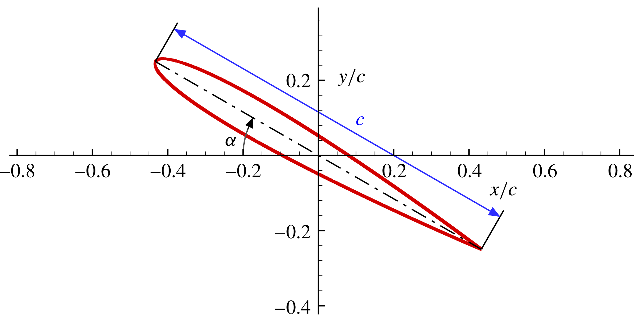
NACA0010 geometry,
 $c$
is the airfoil chord and
 $\unicode[STIX]{x1D6FC}$
the angle of attack.

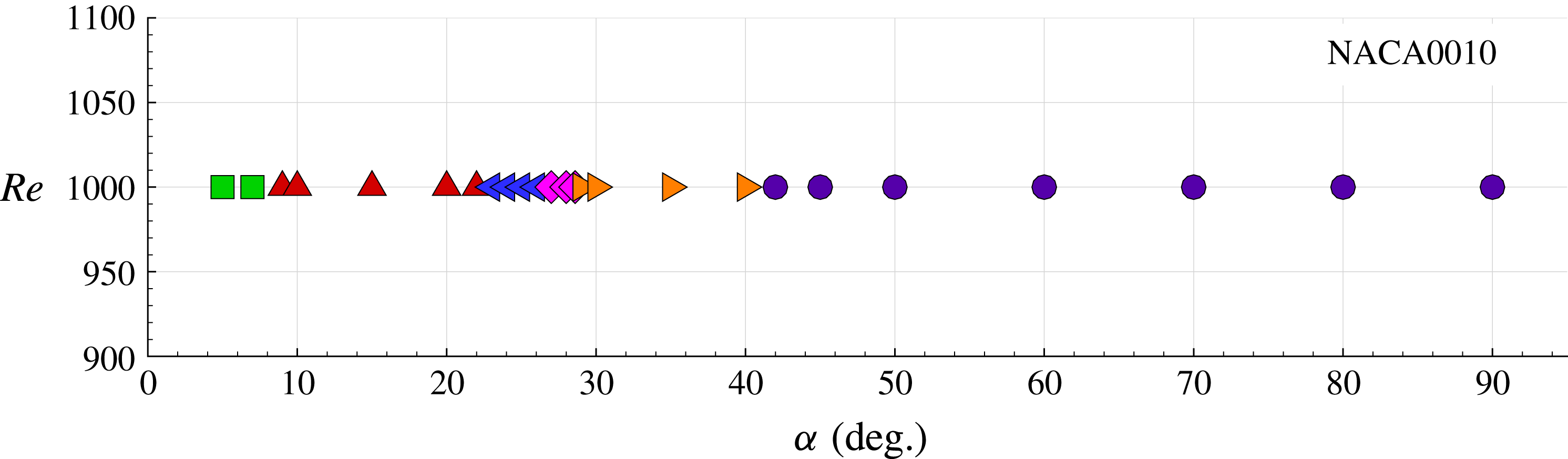
Simulations in the plane
 $Re$
versus
 $\unicode[STIX]{x1D6FC}$
used for revisiting the Kurtulus modes. The different symbols indicate the Kurtulus modes: ▫
 $=$
Mode I, ▵
 $=$
Mode II, ◃
 $=$
Mode IIIa, ♢
 $=$
Mode IV, ▹
 $=$
Mode IIIb, ◯
 $=$
Mode V.

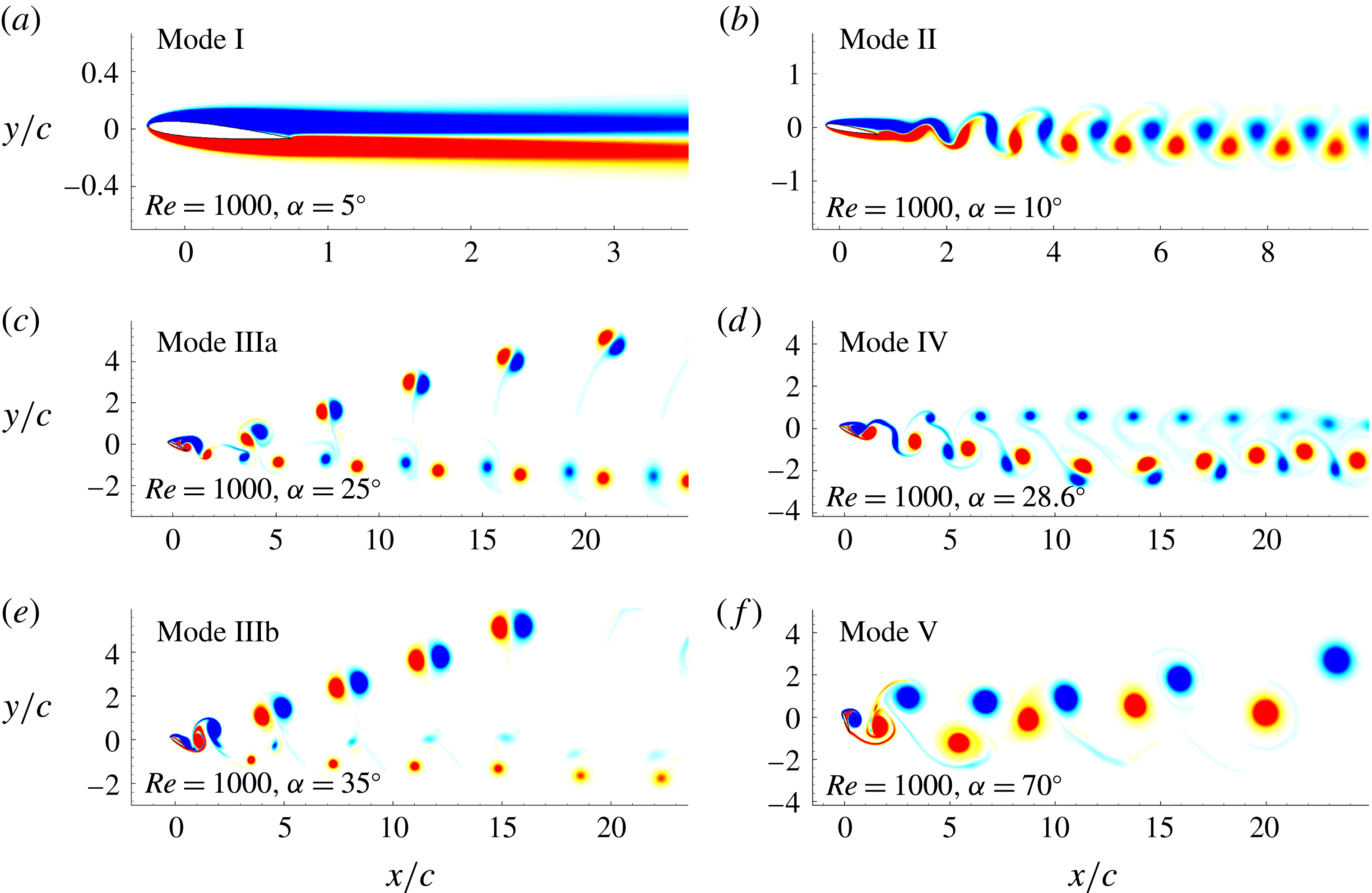
Kurtulus’ modes, for a NACA0010 profile at
 $Re=1000$
, changing the angle of attack
 $\unicode[STIX]{x1D6FC}$
.

In Kurtulus (Reference Kurtulus2016) the wing profiles NACA0002 and NACA0012 were studied at fixed Reynolds number, i.e.
 $Re=1000$
, and changing the angle of attack from
 $0^{\circ }$
to
 $90^{\circ }$
. In this section the same analysis is performed through DVH simulations investigating the flow around the NACA0010 airfoil, also at
 $Re=1000$
. Figure 1 depicts the NACA0010 geometry where
 $c$
denotes the airfoil chord.
Figure 2 reports the different angles of attack used for this first study. The DVH results are quite close to the ones obtained by Kurtulus with the NACA0012. All these NACA profiles are symmetric, they differ only in thickness (NACA0002 is the thinnest one).
In figure 3, DVH vorticity plots are reported for angles of attack
 $\unicode[STIX]{x1D6FC}$
equal to
 $5^{\circ }$
,
 $10^{\circ }$
,
 $25^{\circ }$
,
 $28.6^{\circ }$
,
 $35^{\circ }$
and
 $70^{\circ }$
of the NACA0010, detecting all the five different modes identified by Kurtulus (Reference Kurtulus2016). Here is the description of these modes:
(i) Mode I: ‘Continuous vortex sheet mode’, small angles of attack (
 $\unicode[STIX]{x1D6FC}\in 0^{\circ }{-}8^{\circ }$
). The flow around the airfoil is attached or it is characterized by a stable narrow recirculation zone near the trailing edge. The wake is stable and both lift and drag reach, after a transitory regime, a steady condition.
(ii) Mode II: ‘Alternating vortex shedding mode’, moderate angles of attack (
$\unicode[STIX]{x1D6FC}\in 9^{\circ }{-}22^{\circ }$
). The flow is characterized by the shedding of vortex paired structures in the wake region. Lift and drag forces exhibit a periodic behaviour. Within this mode we enter in the critical region that precedes the stall condition. The forces are almost sinusoidal with a single dominant frequency in their spectra. Increasing the angle of attack towards the upper limit of this range leads to the appearance of the period-doubling phenomenon discussed in Pulliam & Vastano (Reference Pulliam and Vastano1993) and the subsequent transition to Mode IIIa.(iii) Mode IIIa: ‘Alternating vortex pairs shedding mode’, high angles of attack (
$\unicode[STIX]{x1D6FC}\in 23^{\circ }{-}26^{\circ }$
). The wake is characterized by the shedding of series of two distinct vortex pairs moving in two different directions: one pair moves practically in the direction of the free stream velocity while the other one moves upwards. This kind of dynamics makes the wake thicker than in the previous case. The force spectrum presents an increased number of frequency peaks.(iv) Mode IV: ‘Alternating vortex pairs shedding mode in free stream’, high angles of attack (
$\unicode[STIX]{x1D6FC}\in 27^{\circ }{-}28.9^{\circ }$
). Within this narrow range of angles of attack the wake becomes thinner again. Looking at figure 3(d), for
$\unicode[STIX]{x1D6FC}=28.6^{\circ }$
, the wake presents a quite regular pattern with two different sets of vortices: the lower set is formed again by dipoles while the upper one by a row of clockwise vortices. This mode is highly influenced by the airfoil thickness and by the Reynolds number. In particular, for thin airfoils this configuration remains stable for a larger range of
$\unicode[STIX]{x1D6FC}$
. In §§ 3.2 and 3.3 a similar vortex pattern is discussed with an angle
$\unicode[STIX]{x1D6FC}=30^{\circ }$
but reducing the Reynolds number to 900.(v) Mode IIIb: ‘Alternating vortex pairs shedding mode’. The Mode III reappears for higher angles of attack (
$\unicode[STIX]{x1D6FC}\in 29^{\circ }{-}41^{\circ }$
) but in this case the vortex pairs which move upwards are more intense and they move faster in the vertical direction. At the same time, the dipoles moving in the free stream direction are now unbalanced, the anti-clockwise vortices being more intense than the clockwise ones (see figure 3
e).(vi) Mode V: ‘Bluff body vortex shedding mode’, extreme angles of attack (
$\unicode[STIX]{x1D6FC}\in 42^{\circ }{-}90^{\circ }$
). At large incidence the vortex shedding behaves as for a bluff body. Vortices generated on the leading and trailing edges strongly interact with each other before being released into the wake. The vortices grow slowly and the intensity of the vorticity nearby the separation from the sharp trailing edge is more intense than the one from the rounded-shape leading edge.


In figure 2 the modes found for the different AOAs are reported through different symbols.
In the analysis performed in Kurtulus (Reference Kurtulus2016) it is clearly shown that the transition from Mode III to Mode IV is characterized by a bifurcation of the solution. Because this phenomenon appears for both the airfoils NACA0002 and NACA0012, the results obtained are not strictly connected with the specific airfoil used. Combining our results with the ones obtained by Kurtulus, we see that the range of existence of the different modes changes. A similar behaviour is discussed in §§ 3 and 4 considering the NACA0010 and an elliptical profiles at angle of attack
 $\unicode[STIX]{x1D6FC}=30^{\circ }$
and changing the Reynolds number from 100 up to 3000.
3 Flow around a NACA0010 airfoil for different Reynolds numbers with angle of attack
$\unicode[STIX]{x1D6FC}=30^{\circ }$

In this section the flow around a NACA0010 airfoil with angle of attack
 $\unicode[STIX]{x1D6FC}=30^{\circ }$
is considered whilst varying the Reynolds number within the range
 $Re=100$
to
 $Re=3000$
.
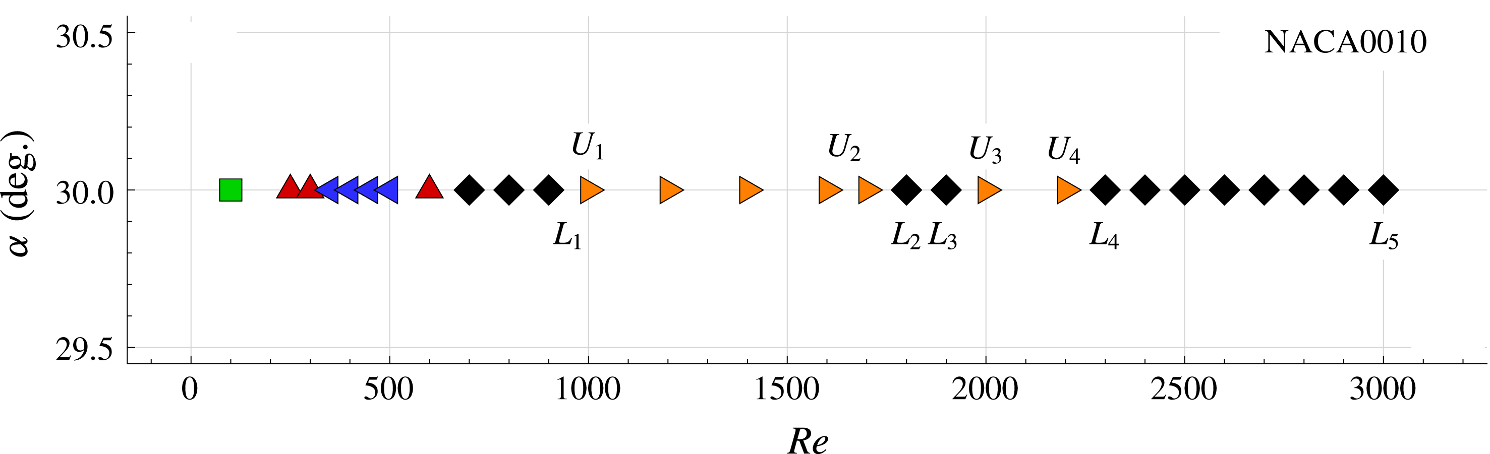
In figure 4 the Reynolds numbers of the studied cases are depicted and the symbols for each Reynolds number indicate the different Kurtulus’ modes, in analogy with figure 2, but with fixed AOA and variable
 $Re$
this time. The labels
 $L_{1}$
,
 $U_{1}$
. indicate cases which will be further discussed in this section, between which sudden changes of mode occur.
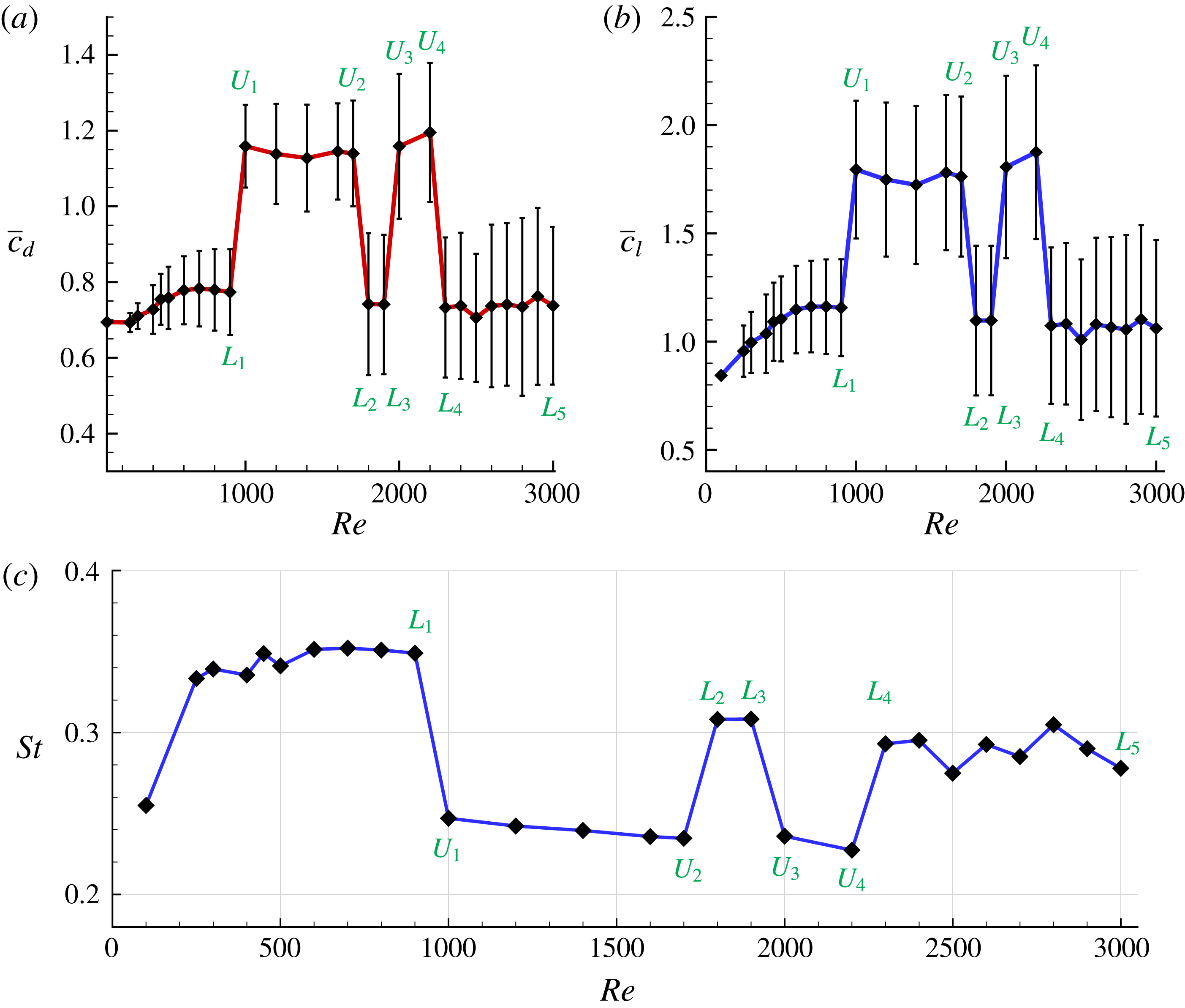
Figure 5(a,b) shows the mean values and standard deviations of the lift and drag components, evaluated after the transitory stages. In figure 5(c) the evolution of Strouhal number (
 $St$
) versus
 $Re$
is depicted. The evaluation of the Strouhal number is performed from a Fourier analysis of the lift time signal, considering the frequency of the fundamental harmonic component of the spectrum. In all these plots, bifurcations of the solution at specific Reynolds numbers are well visible. Two branches can be identified in terms of mean lift/drag:
(i) a lower branch, denoted by
$L$
, corresponding to cases with mean drag coefficient
$\bar{c}_{d}\approx 0.75$
and mean lift coefficient
$\bar{c}_{l}\approx 1$
, including in particular cases
$L_{1}$
to
$L_{5}$
, and(ii) an upper branch, denoted by
$U$
, corresponding to cases with mean drag coefficient
$\bar{c}_{d}\approx 1.2$
and mean lift coefficient
$\bar{c}_{l}\approx 1.75$
, including in particular cases
$U_{1}$
to
$U_{4}$
.


Test matrix in the plane
 $\unicode[STIX]{x1D6FC}$
versus
 $Re$
used for the flow analysis. The different symbols indicate the Kurtulus modes: ▫
 $=$
Mode I, ▵
 $=$
Mode II, ◃
 $=$
Mode IIIa, ♢
 $=$
Mode IV, ▹
 $=$
Mode IIIb, ◯
 $=$
Mode V.

NACA0010 with angle of attack
 $\unicode[STIX]{x1D6FC}=30^{\circ }$
. (a,b) Mean drag (a) and lift (b) coefficients versus
 $Re$
(error bars indicate the standard deviation). (c) Strouhal number versus
 $Re$
.

The four bifurcations identified for the NACA0010 appear in the following order:
(i) first bifurcation, between
$Re=900$
(case
$L_{1}$
) and
$Re=1000$
(case
$U_{1}$
);(ii) second bifurcation, between
$Re=1700$
(case
$U_{2}$
) and
$Re=1800$
(case
$L_{2}$
);(iii) third bifurcation, between
$Re=1900$
(case
$L_{3}$
) and
$Re=2000$
(case
$U_{3}$
);(iv) fourth bifurcation, between
$Re=2200$
(case
$U_{4}$
) and
$Re=2300$
(case
$L_{4}$
).


The following discussion is organized into four parts. First, in § 3.1, we discuss the changes of modes found before the first bifurcation. Second, in § 3.2, we discuss the discovered bifurcations in terms of common characteristics of the cases belonging, respectively, to the lower and upper branches. Third, in § 3.3, some peculiarities of the different cases studied are also noted. Last, in § 3.4, we investigate the near field close to the upper part of the airfoil in terms of vortical structures, detachments and reattachments and pressure profiles on the airfoil. Links are also made between the vortical evolution of the flow near the upper part of the airfoil and the wake structure observed downstream, when crossing a bifurcation.
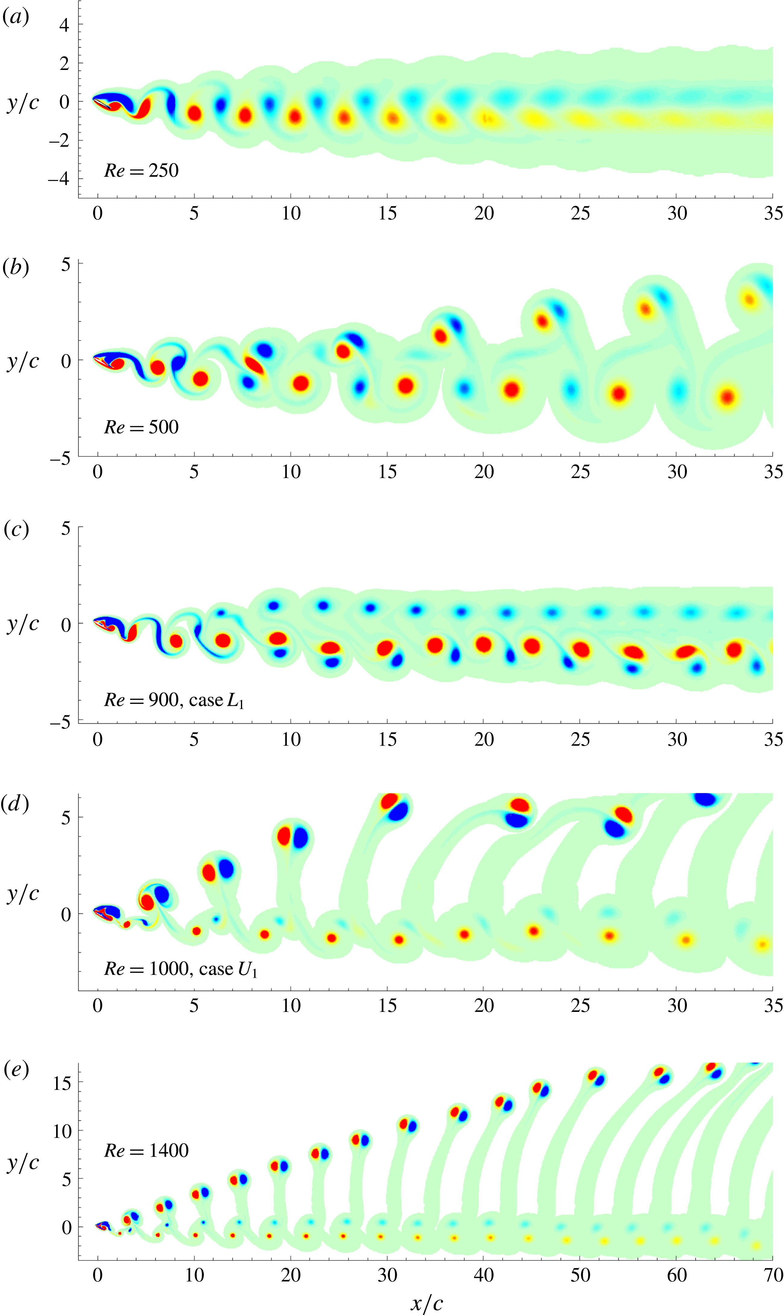
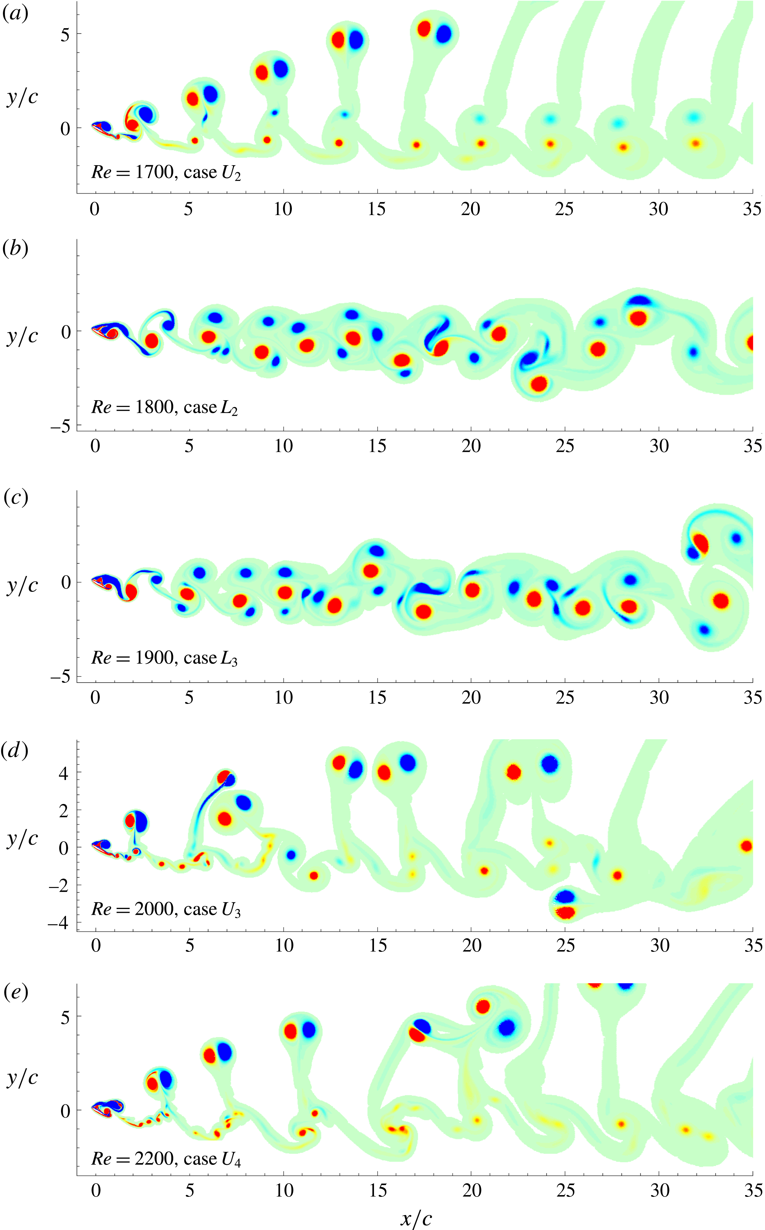
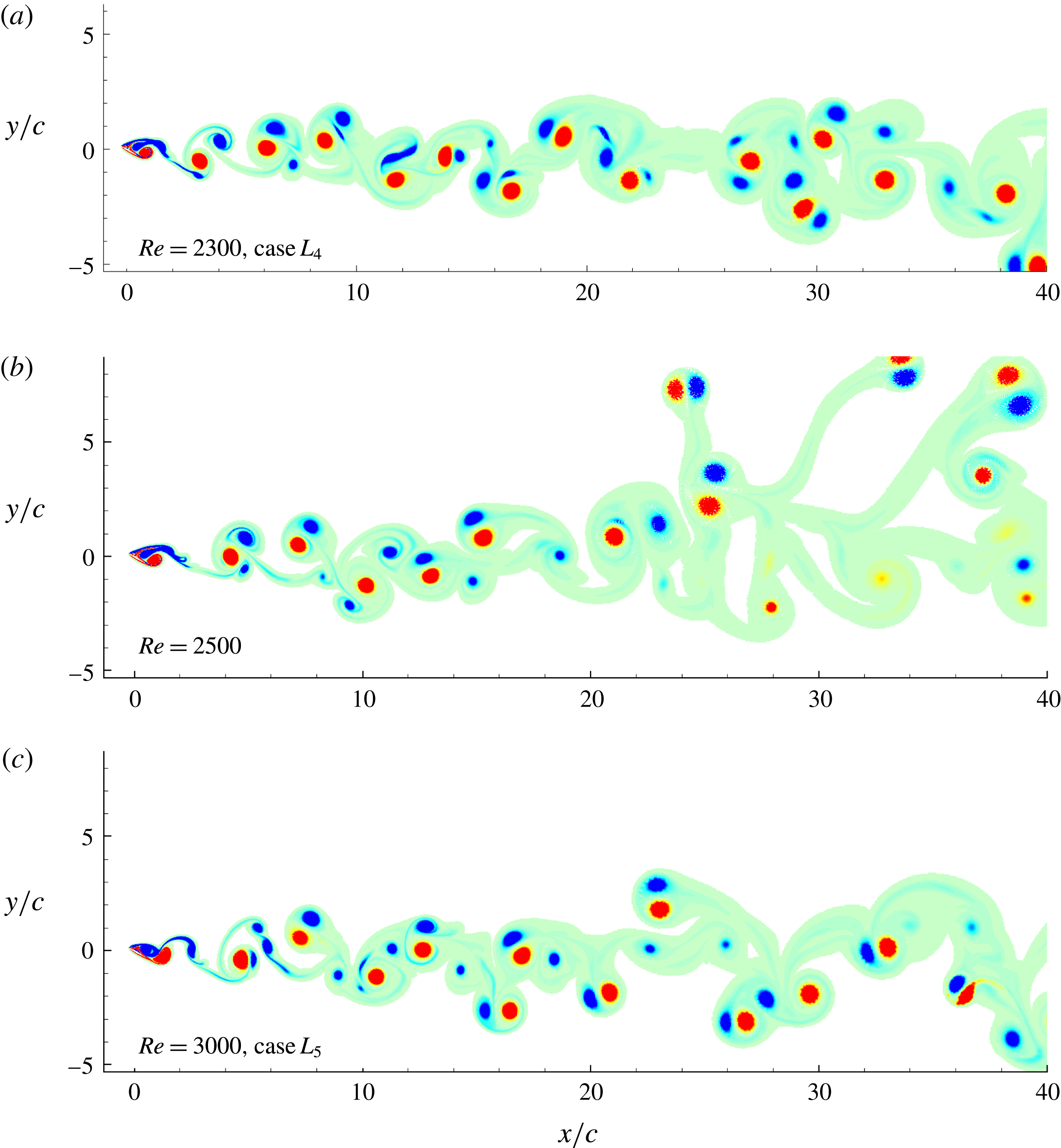
In order to these discussions of the different behaviours of the flow and of the forces acting on the airfoil when changing the Reynolds number, 12 cases are selected and the results presented in the following figures are used:
(i) Figure 6 depicts the wake structures for
$Re=250$
, 500, 900, 1000 and 1400.(ii) Figure 7 depicts the wake structures for
$Re=1700$
, 1800, 1900, 2000 and 2200.(iii) Figure 8 depicts the wake structures for
$Re=2300$
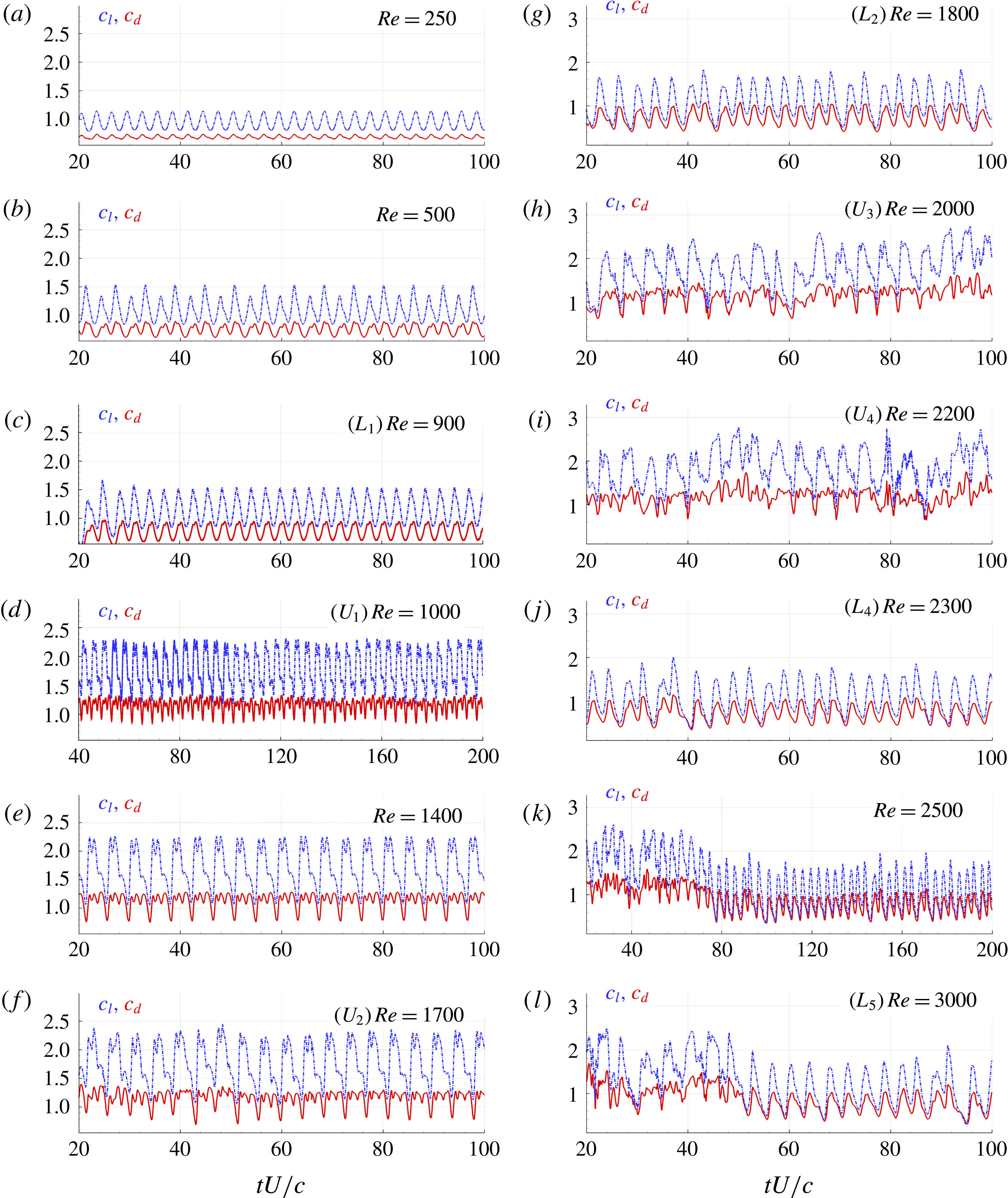
, 2500 and 3000.(iv) Figure 9 reports the time histories of lift and drag coefficients for these 12
$Re$
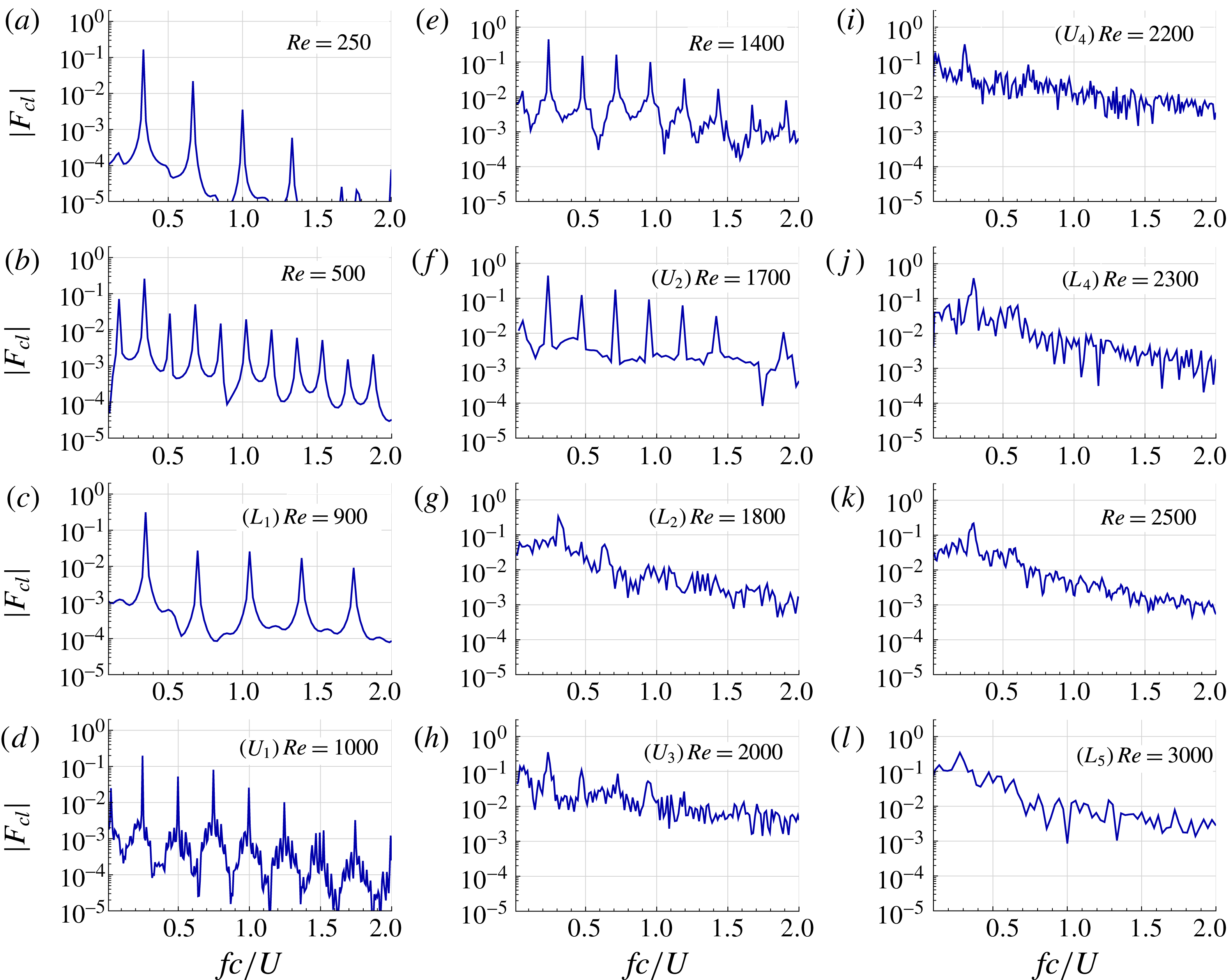
.(v) Figure 10 shows the Fourier coefficients of the lift force for the same 12 cases.
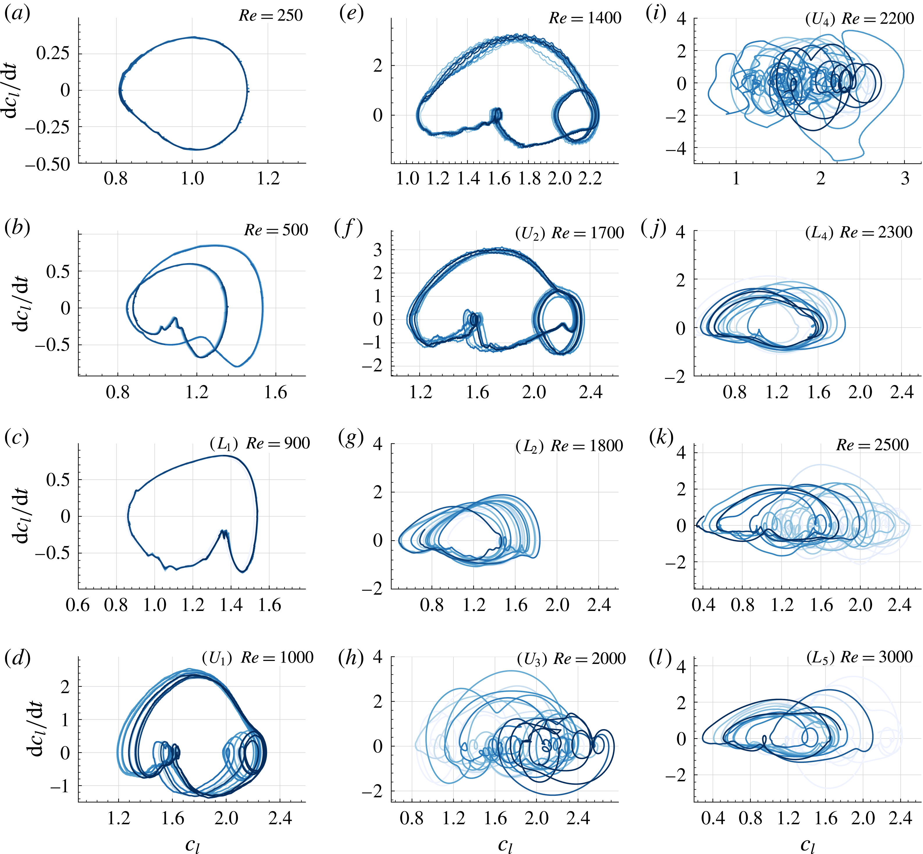
(vi) Figure 11 displays Poincaré maps of lift coefficient versus its time derivative for the same 12 cases. With this figure we follow the analysis of Khalid & Akhtar (Reference Khalid and Akhtar2012) where Poincaré maps are used to study the nonlinear behaviour of a NACA0012 airfoil at
$Re=1000$
varying the angle of attack.


Wakes shedding downstream of a NACA0010 profile with angle of attack
 $\unicode[STIX]{x1D6FC}=30^{\circ }$
for
 $Re$
numbers equal to: 250, 500, 900, 1000 and 1400. All the cases are shown at non-dimensional time
 $tU/c=100$
. Vorticity contour plots range from
 $\unicode[STIX]{x1D714}c/U=-2$
to
 $2$
. See supplementary movie 1 available at https://doi.org/10.1017/jfm.2018.189 for the case
 $Re=900$
.

Wakes shed by a NACA0010 profile with angle of attack
 $\unicode[STIX]{x1D6FC}=30^{\circ }$
for
 $Re$
numbers equal to: 1700, 1800, 1900, 2000, 2200. All the cases are shown at non-dimensional time
 $tU/c=100$
. Vorticity contour plots range from
 $\unicode[STIX]{x1D714}c/U=-2$
to
 $2$
.

3.1 Changes of modes before the first bifurcation: passing from single frequency periodic to period doubling
We recall that in this section, contrary to the previous one, the AOA
 $\unicode[STIX]{x1D6FC}$
is fixed and
 $Re$
varies.
For the lowest
 $Re$
studied, equal to 100, Mode I is obtained: the viscosity level is so high that the flow practically does not separate. Time histories of the loads do not present relevant unsteadiness, after the transitory stage.
At
 $Re=250$
Mode II is obtained: although the angle of attack is high and the inertia is expected to be dominant, the viscous forces are intense enough to induce a regular shedding mechanism past the airfoil. This is well visible in figure 6(a), where the vorticity pattern released by the NACA0010 is depicted. The von Kármán vortex street remains stable in the wake of the airfoil, during the whole simulation time. The drag and lift forces oscillate periodically in time (see figure 9
a). Figure 10(a) shows the Fourier coefficients of the lift force signal. From this spectrum, a fundamental harmonic at frequency
 $f_{1}\simeq 1/3\,U/c$
can be easily identified. Other harmonics with frequencies of
 $2f_{1}$
,
 $3f_{1}$
and
 $4f_{1}$
are also visible, even if their intensities are increasingly smaller. The periodicity of the lift force is also confirmed by figure 11(a), where the Poincaré map of lift coefficient versus its time derivative shows a stable orbit.
Wakes shed by a NACA0010 profile with angle of attack
 $\unicode[STIX]{x1D6FC}=30^{\circ }$
for
 $Re$
numbers equal to 2300 (a), 2500 (b) and 3000 (c). All the cases are shown at non-dimensional time
 $tU/c=100$
. Vorticity contour plots range from
 $\unicode[STIX]{x1D714}c/U=-2$
to
 $2$
.

Time histories of the forces coefficients
 $c_{l}$
(dash-dotted lines) and
 $c_{d}$
(solid lines) for 12 different
 $Re$
numbers.

Modulus of the Fourier coefficients of lift time signals for 12 different
 $Re$
numbers.

Poincaré maps
 $c_{l}$
versus
 $\text{d}c_{l}/\text{d}t$
for 12 different
 $Re$
numbers.

Increasing the Reynolds number up to
 $Re=500$
, the airfoil wake suddenly changes, passing from Mode II to Mode IIIa, see figure 6(b), even though no bifurcation in the mean lift/drag or Strouhal number occurs. An interesting feature of this mode can be seen from the analysis of the Fourier coefficients of the lift force. Actually, the spectrum in figure 10(b) shows that the main harmonics duplicate with respect to the previous case: within the range
 $fc/U\in (0,1)$
there are now six peaks instead of three. This period-doubling mechanism is also reflected on the map reported in figure 11(b), where two entangled orbits appear. The main frequency is
 $f_{1}\simeq 0.341U/c$
, a little higher than the one related to the case
 $Re=250$
. Besides this, a lower-frequency peak is now present at
 $f_{1}/2$
; this sub-harmonic component is clearly visible on the lift coefficient time history (see figure 9
b).
Moving from
 $Re=500$
up to
 $Re=900$
, the Mode IIIa and the period-doubling phenomenon disappear while the Mode IV progressively develops, still without any bifurcation in mean lift/drag or Strouhal number.
3.2 The discovered bifurcations (fixing
$\unicode[STIX]{x1D6FC}$
and changing
$Re$
): common characteristics


As depicted in figure 5 we have discovered four bifurcations at fixed AOA of
 $30^{\circ }$
, which all occur in the range
 $Re=\in (900,2300)$
. Each bifurcation is characterized by a sudden jump in mean lift/drag coefficients and
 $St$
. As can be seen in figure 5(a,b), at each bifurcation the mean lift/drag coefficients jump from a lower branch to an upper branch, or the other way round. As mentioned before, each branch is characterized by values of these mean coefficients which have only small variations in the range of
 $Re$
studied. Namely, the mean drag and lift are approximately equal to
 $0.75$
and
 $1.0$
, respectively, for the lower branch, while they are approximately
 $\bar{c}_{d}\approx 1.2$
and
 $\bar{c}_{l}\approx 1.75$
for the upper branch. In terms of
 $St$
, it can be seen in the bottom panel of the same figure that the branches are inverted: the lower one (in terms of mean lift/drag) is characterized by
 $St$
greater than
 $0.26$
while the upper branch is characterized by values lower than
 $0.26$
.
In terms of wakes, it can be noted that these 4 bifurcations all occur between Modes IIIb (upper branch) and IV (lower branch), as can be seen in figure 4. This means that the wakes exhibit common features in cases
 $L_{1}$
,
 $L_{2}$
,
 $L_{3}$
,
 $L_{4}$
on the one hand, and
 $U_{1}$
,
 $U_{2}$
,
 $U_{3}$
,
 $U_{4}$
on the other hand, see figures 6–8. In particular, the two different sets of dipoles of Mode IIIb are present in all upper-branch cases, while they are not present in the lower-branch ones. Besides, contrary to changes of modes for
 $Re<900$
, these large changes in the wake are now associated with bifurcations in mean lift/drag coefficients, see figure 5(a,b).
These bifurcations also occur in terms of
 $St$
, see figure 5(c). Actually, Mode IIIb requires larger time scales for the formation of the vortical structures than Mode IV, leading to Strouhal numbers
 ${\approx}35\,\%$
higher for the lower branch (Mode IV) than the upper one (Mode IIIb). A similar frequency downward shifting of approximately
 $29\,\%$
was also found in the analysis performed in Kurtulus (Reference Kurtulus2015).
When looking at time evolutions of the lift and drag coefficients, see figure 9, one can observe that upper-branch cases of bifurcations are characterized by more complex signals, much less symmetric in time within a given period. In particular, a double maximum is typically observed in each period for the lift, as well as a small oscillation during the lift decrease phase of each period. The more regular behaviour of the lower-branch case signals can be linked to the more regular and less complex vortex shedding of Mode IV than of Mode IIIb, as mentioned above.
These differences in the time evolution of the lift induce, in turn, differences in the Fourier transforms and
 $c_{l}$
–
 ${\dot{c}}_{l}$
Poincaré maps. In particular, the double maximum observed previously within each lift coefficient period of upper-branch cases makes appear a characteristic secondary orbit in the
 $c_{l}$
–
 ${\dot{c}}_{l}$
maps of figure 11, in the right parts (highest lifts) of the plots. Lower-branch bifurcation cases
 $L_{1}$
to
 $L_{4}$
are characterized by simpler and more regular orbits. As for the Fourier coefficients of the lift time signals, it can be noted in figure 10 that small oscillations appear between the different dominant frequencies for the cases
 $U_{1}$
to
 $U_{4}$
, which are not present for the lower-branch bifurcation cases.
Another rather obvious aspect is that, generally, when going to higher and higher Reynolds, due to the appearance of smaller structures, the flow becomes more and more complex, see figures 6–8. Thus the instantaneous lift/drag coefficients become also less regular and less periodic, see figure 9. As a consequence, whereas harmonic components are well visible in the lift coefficient Fourier transform for the first bifurcation, they tend to disappear for the next ones for which the signals are noisier, see figure 10. In turn, the
 $c_{l}$
–
 ${\dot{c}}_{l}$
Poincaré maps present less and less stable forms, both in terms of geometric complexity (regularity) and of stability in position of the orbit (periodicity), see figure 11. In terms of
 $St$
, after the first bifurcation a continuous decrease is observed as
 $Re$
increases both in the lower and in the upper branches (see figure 5), reflecting the fact that the increasing complexity of the flow structures induces larger and larger characteristic times of the periodic wake.
Finally, it is worth noting that we carefully checked that these discovered bifurcations are not influenced by (or originating from) the numerical solver itself. Actually, we performed the same simulations for the first bifurcation
 $L_{1}$
–
 $U_{1}$
using a totally different numerical solver (called WCCH) based on:
(i) the mesh-based finite volume method instead of a particle vortex method,
(ii) a weakly compressible approach instead of an incompressible one,
(iii) the immersed-boundary method instead of a body-fitted one,
and the results of the two solvers are in very close agreement, as commented more in detail in the appendix A of this article.
3.3 Peculiarities of some of the cases simulated in the bifurcations Reynolds range
3.3.1
$Re=900$
– Case
$L_{1}$
before the first bifurcation


This case is one of the most regular of all the cases simulated, as is visible both in the time evolution of the drag/lift coefficient in figure 9(c) and on the
 $c_{l}{-}{\dot{c}}_{l}$
map in figure 11(c). It is characterized by a fundamental component of frequency mode
 $f_{1}$
(see figure 10
c), corresponding to
 $St=f_{1}c/U=0.35\,$
which is one of the highest Strouhal numbers recorded for all the cases studied (see figure 5). Higher-frequency components,
 $2f_{1},3f_{1},\ldots$
, with lower intensities, are also well visible in the lift Fourier coefficients.
3.3.2
$Re=1000$
– Case
$U_{1}$
after the first bifurcation


As mentioned before, the Fourier coefficients of the lift force for this case belonging to the upper branch are characterized by a down-shifted fundamental frequency component
 $f_{1}\simeq 1/4\,U/c$
(see figure 10
d). It can be noticed also that, besides the harmonic frequency components well visible as for the case
 $L_{1}$
, a low-frequency modulation of approximately
 $f_{1}/9$
is present in this case indicating a slow dynamics of the wake. This modulation is clearly visible as well in the
 $c_{l}{-}{\dot{c}}_{l}$
map of figure 11(d) where the orbit position oscillates.
3.3.3
$Re=1400$

For this case, as for case
 $L_{1}$
, a very regular solution is found, much more periodic than close-by cases
 $U_{1}$
or
 $U_{2}$
of the same branch. This regularity in time well is visible in figures 9(e), 10(e) and 11(e) may be related to the one of the wake. Actually, in figure 6(e) one can observe that dipoles move straight upward with very balanced positive and negative vorticity. As a consequence, they are positioned on an almost straight oblique line.
3.3.4
$Re=1800$
– case
$L_{2}$
after the second bifurcation


From this case on, the vorticity pattern is no longer regular, as clearly visible in figure 7(b), and there is no more close resemblance with the modes described in Kurtulus (Reference Kurtulus2016). However, the wake remaining confined within a thickness of approximately six times the airfoil chord as in case
 $L_{1}$
, it can still be classified as Mode IV. This remark is also valid for higher-
 $Re$
cases of the lower branch:
 $L_{3}$
up to
 $L_{5}$
. Nota bene, case
 $L_{3}$
is very similar to case
 $L_{2}$
so that it has not been displayed in figures 9–11.
As expected this change in the vorticity field induces changes in the time behaviour of the lift and drag forces, which are less and less periodic, see figure 9. In turn, for this case and higher Reynolds ones the only frequency clearly recognizable in the Fourier spectra is the one linked to the vortex shedding, see figure 10, and unstable orbits are found in the plane
 $c_{l}{-}{\dot{c}}_{l}$
, see figure 11. One can also notice that the mean lift and drag coefficients for this case
 $L_{2}$
have values close to the ones of case
 $L_{1}$
, while the Strouhal number shows a decrease of approximately
 $12\,\%$
between these two cases, see figure 5.
3.3.5
$Re=2500$
and
$3000$
– after the fourth bifurcation


For these higher Reynolds cases, the wake structure resembles the one of cases
 $L_{2}$
,
 $L_{3}$
and
 $L_{4}$
, in the sense that the different vortex structures remain confined, see figures 7 and 8. However, differently from these cases, some dipoles have the tendency to exit the main wake region, as depicted by figure 8(b,c).
Besides the irregularities of the force components observed as for the previous cases, see figure 9, one can note a change of behaviour in time after, respectively,
 $t=80c/U$
and
 $t=50c/U$
seconds for cases
 $Re=2500$
and 3000, indicating a bifurcation of the solution in time from Mode IIIb to Mode IV. There is thus a long transient phase in Mode IIIb before reaching the established Mode IV. This can also be observed looking at the wake of, e.g. case
 $Re=2500$
, where the two regimes are visible: Mode IIIb for
 $x>20c$
and Mode IV for
 $x<20c$
(see figure 8
b).
3.4 Analysis of the near field when crossing the bifurcations
The cases studied in the previous section are considered again here, focusing this time on the near field, especially in terms of vorticity. In order to investigate the effects of the bifurcation phenomena on the local loads of the airfoil, a mean body pressure coefficient
 $\bar{c}_{p}$
is also evaluated.
For the sake of brevity only the first three bifurcations will be analysed in this section, i.e. cases
 $L_{1}{-}U_{1}$
,
 $U_{2}{-}L_{2}$
and
 $L_{3}{-}U_{3}$
.
Finally, in § 3.4.3 a detailed description of the near field is performed for the Mode III and the Mode IV cases within a period of the lift force. Nine time instants are considered linking the instantaneous streamlines of the velocity fields with the instantaneous pressure profile calculated on the suction side of the airfoil.
3.4.1 Near body vorticity field
The near body vorticity field and streamlines for the first three bifurcations
 $L_{1}{-}U_{1}$
,
 $U_{2}{-}L_{2}$
,
 $L_{3}{-}U_{3}$
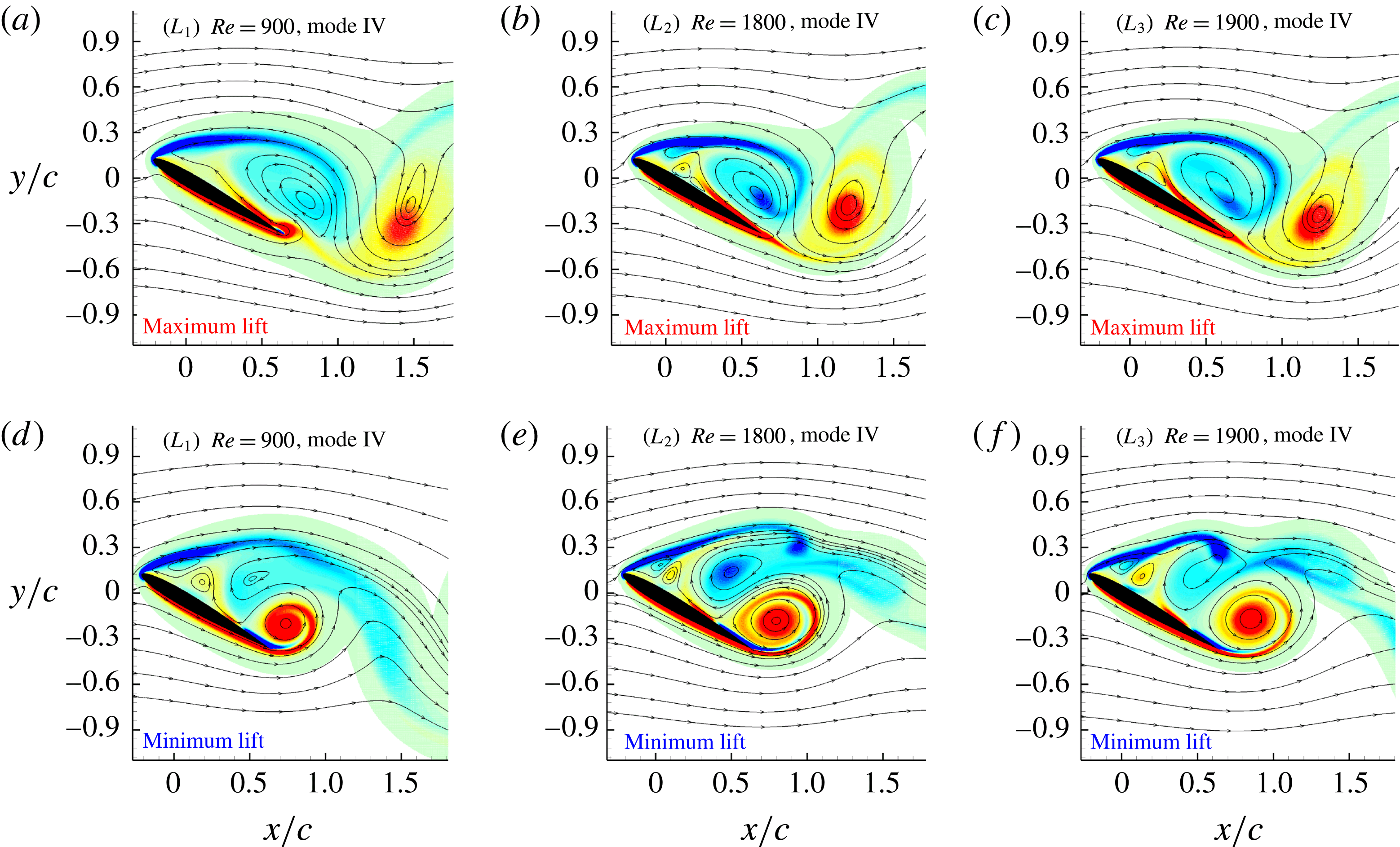
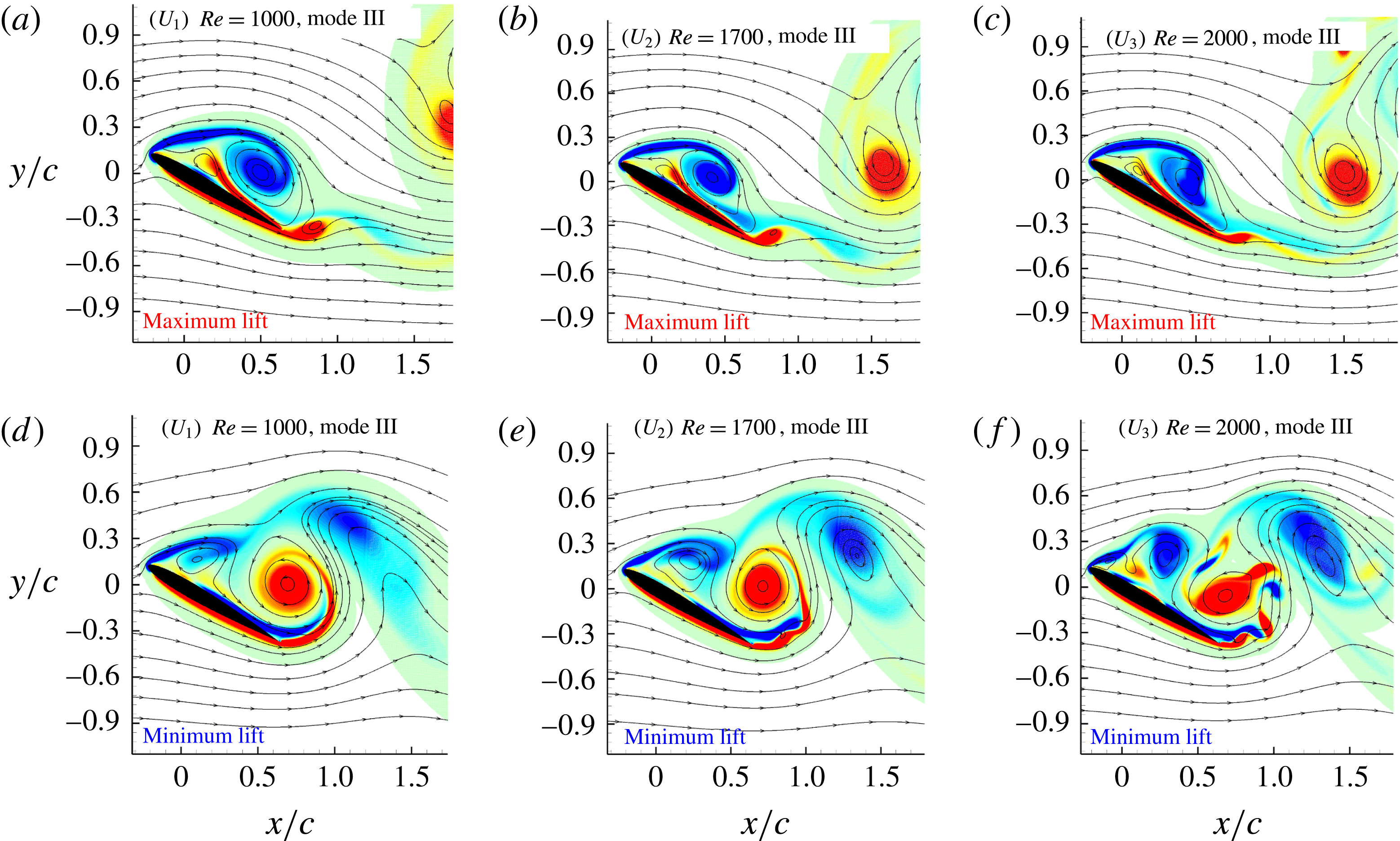
are depicted in figures 12 and 13. For each Reynolds number two snapshots were taken: one at the maximum of the lift and the other at its minimum.
To highlight the common behaviours at different Reynolds numbers, figure 12 shows snapshots of cases
 $L_{1}$
,
 $L_{2}$
and
 $L_{3}$
which are characterized by the Mode IV, while figure 13 concerns cases
 $U_{1}$
,
 $U_{2}$
and
 $U_{3}$
characterized by the Mode IIIb.
At the maximum of the lift (figures 12
a–c, 13
a–c), all of these cases present a clockwise shear layer shed by the leading edge of the airfoil generating a recirculation zone which extends almost for all the length of the airfoil. For cases
 $L_{1}$
,
 $L_{2}$
and
 $L_{3}$
(Mode IV) the recirculation zone appears larger than for the cases
 $U_{1}$
,
 $U_{2}$
and
 $U_{3}$
(Mode IIIb). For
 $U_{1}$
,
 $U_{2}$
and
 $U_{3}$
, even if the recirculation zone is smaller, the vorticity of the shear layer is clearly more intense. This main difference will lead to a completely different wake behaviour associated with Mode IV and Mode III.
Near body vorticity field and streamlines taken at the maximum (upper row) and the minimum (lower row) of the lift force. Dimensionless vorticity field
 $\unicode[STIX]{x1D714}c/U$
scales from
 $-15$
(blue) to 15 (red).

Near body vorticity field and streamlines at the maximum (upper row) and the minimum (lower row) of the lift force. Dimensionless vorticity field
 $\unicode[STIX]{x1D714}c/U$
scales from
 $-15$
(blue) to 15 (red).

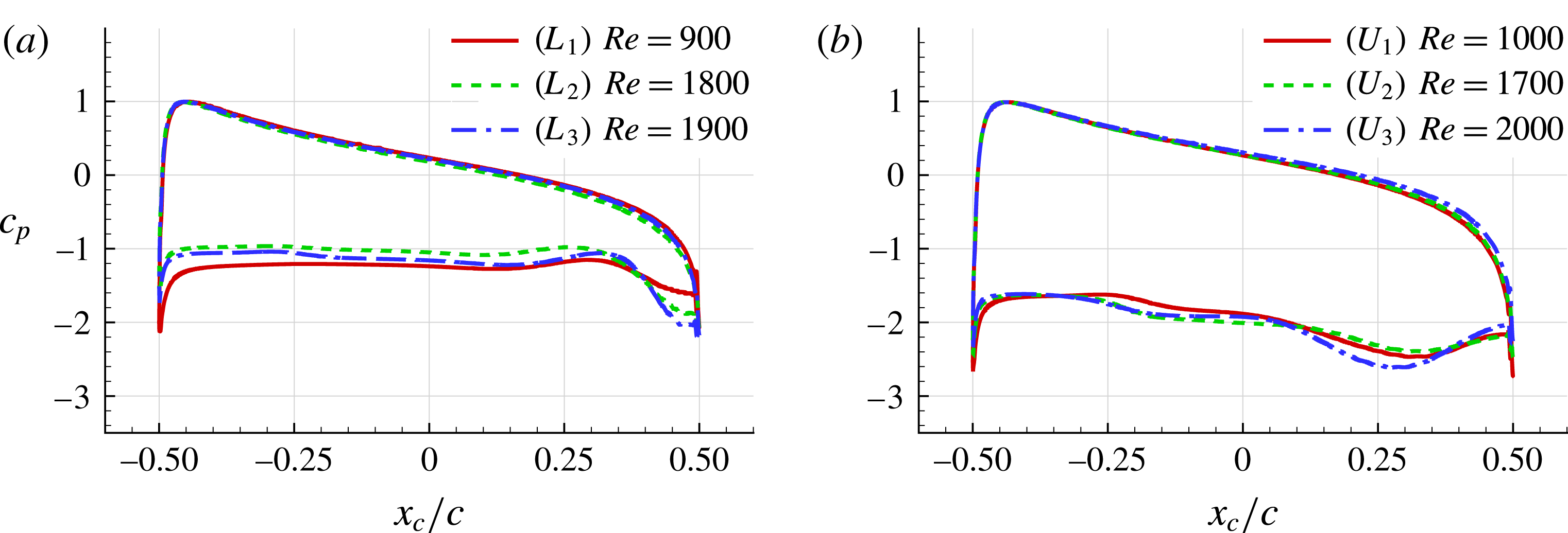
Mean pressure coefficient distribution: (a) cases
 $L_{1}$
–
 $L_{2}$
–
 $L_{3}$
, (b) cases
 $U_{1}$
–
 $U_{2}$
–
 $U_{3}$
.

At the maximum lift instant for cases
 $L_{1}$
,
 $L_{2}$
and
 $L_{3}$
, the leading and trailing-edge vortices are interacting, forming a dipole structure which does not present a relevant vertical velocity component. As a result in the Mode IV the wake remains quite compact and narrow with respect to what happens in Mode IIIb. At the minimum lift instant for cases
 $L_{1}$
,
 $L_{2}$
and
 $L_{3}$
, the shear-layer shed by the trailing edge is swallowed up on the suction side with a strong anti-clockwise roll-up mechanism while the leading-edge shear layer is pushed upward.
For cases
 $U_{1}$
,
 $U_{2}$
and
 $U_{3}$
(figure 13) a similar behaviour takes place. However, at the maximum lift instant, the intense clockwise shear layer detached from the leading edge starts to roll-up inducing the generation of an upstream current with positive vorticity on the profile. At the minimum lift instant, the trailing-edge shear layer is swallowed up on the suction side with larger intensity with respect to cases
 $L_{1}$
,
 $L_{2}$
,
 $L_{3}$
. As a result the leading and trailing-edge shear layers interact and a dipole structure is formed and detached in the wake with a substantial upward velocity component.
It must be noticed that for the case
 $U_{3}$
the Reynolds number is high enough to allow the fragmentation of the shear layer detached from the trailing edge. Consequently a chain of small eddies is formed, orbiting and merging with the main trailing-edge vortex, as shown in figure 13(f).
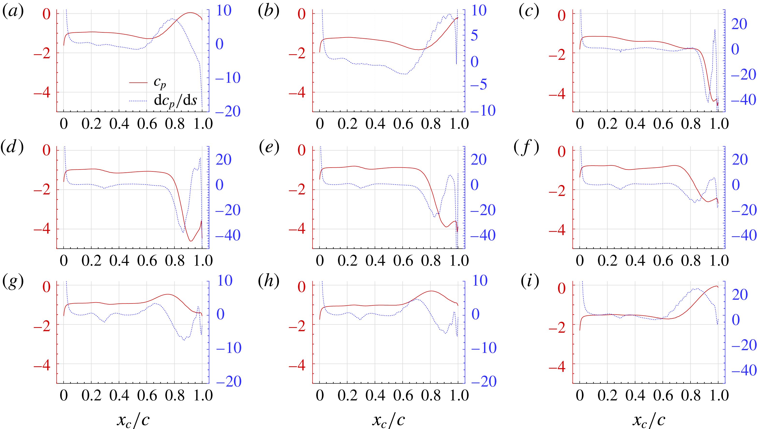
3.4.2 Mean body pressure coefficient analysis
In this section, the mean pressure coefficient
 $\bar{c}_{p}$
distribution on the body is evaluated, using at least 100 samples for each shedding period. In the following results, the
 $x_{c}$
coordinate is the position along the chord of the airfoil with
 $x_{c}=0$
taken at the centre of the chord.
As shown in figure 14, the
 $\bar{c}_{p}$
distributions related to cases
 $L_{1}$
,
 $L_{2}$
and
 $L_{3}$
present strong similarities in the pressure profiles, all these cases belonging to the Mode IV. A comparable similarity is also visible for the cases
 $U_{1}$
,
 $U_{2}$
and
 $U_{3}$
related to the Mode III.
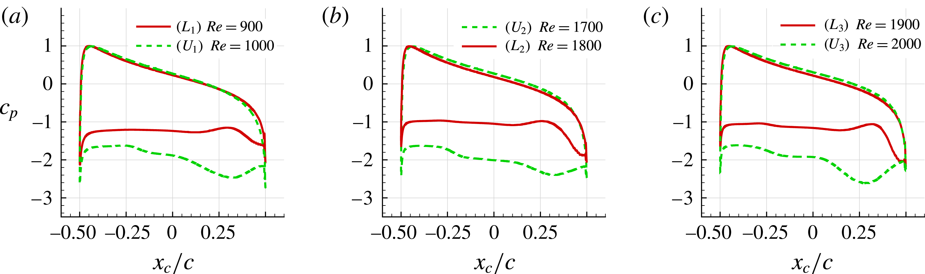
Figure 15 compares the pressure coefficient distributions for the three bifurcations:
 $L_{1}{-}U_{1}$
,
 $U_{2}{-}L_{2}$
and
 $L_{3}{-}U_{3}$
. As evident, the Mode IV (
 $L_{1}$
–
 $L_{2}$
–
 $L_{3}$
) is characterized by an higher pressure distribution on the suction side. Conversely, the more intense vortical evolutions of the near field for Mode III (
 $U_{1}$
–
 $U_{2}$
–
 $U_{3}$
) induce stronger depression visible in the dashed-line curves in plots of figure 15.
3.4.3 Inspection of the near-field vortex dynamics for the second bifurcation cases, along one period of lift oscillation
In this section a more in depth analysis of the near-field flow is conducted for the Modes III and IV. Indeed, to fully identify the mechanisms related to the two modes it is not enough to consider just the instants related to the minimum and maximum lift, but we need to follow the different stages within one period of the lift oscillations. For the sake of brevity we consider only the cases
 $U_{2}\,(Re=1700)$
and
 $L_{2}\,(Re=1800)$
corresponding to the second bifurcation.
In the following analysis the approach by Anand & Sarkar (Reference Anand and Sarkar2017) is also used. The latter is based on the use of the pressure profile on the airfoil suction side and its spatial derivative to identify the positions of separations and reattachments of the shear layers. The DVH method used for the simulations presented in this work allows for an accurate evaluation of pressure profiles on the airfoil (see, e.g. Rossi et al. Reference Rossi, Colagrossi, Bouscasse and Graziani2015a ). Furthermore, as shown in Colagrossi, Graziani & Pulvirenti (Reference Colagrossi, Graziani and Pulvirenti2014), the spatial derivative of the pressure profile can be directly evaluated with this vortex method.
Mean pressure coefficient distribution: (a) first bifurcation (cases
 $L_{1}$
and
 $U_{1}$
), (b) second bifurcation (cases
 $U_{2}$
and
 $L_{2}$
), (c) third bifurcation (cases
 $L_{3}$
and
 $U_{3}$
).

Case
$U_{2}$
- Mode IIIb

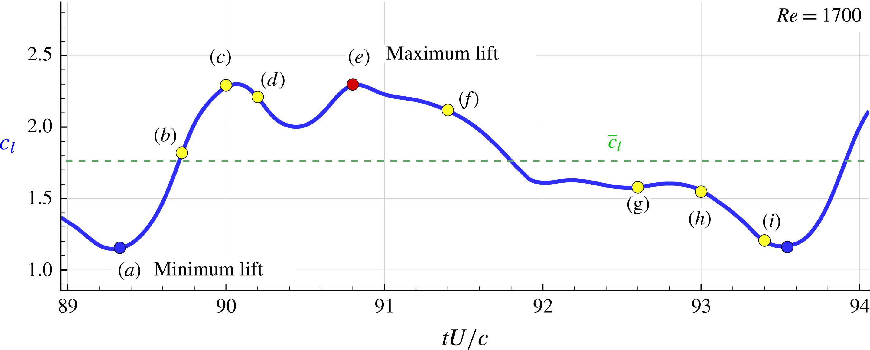
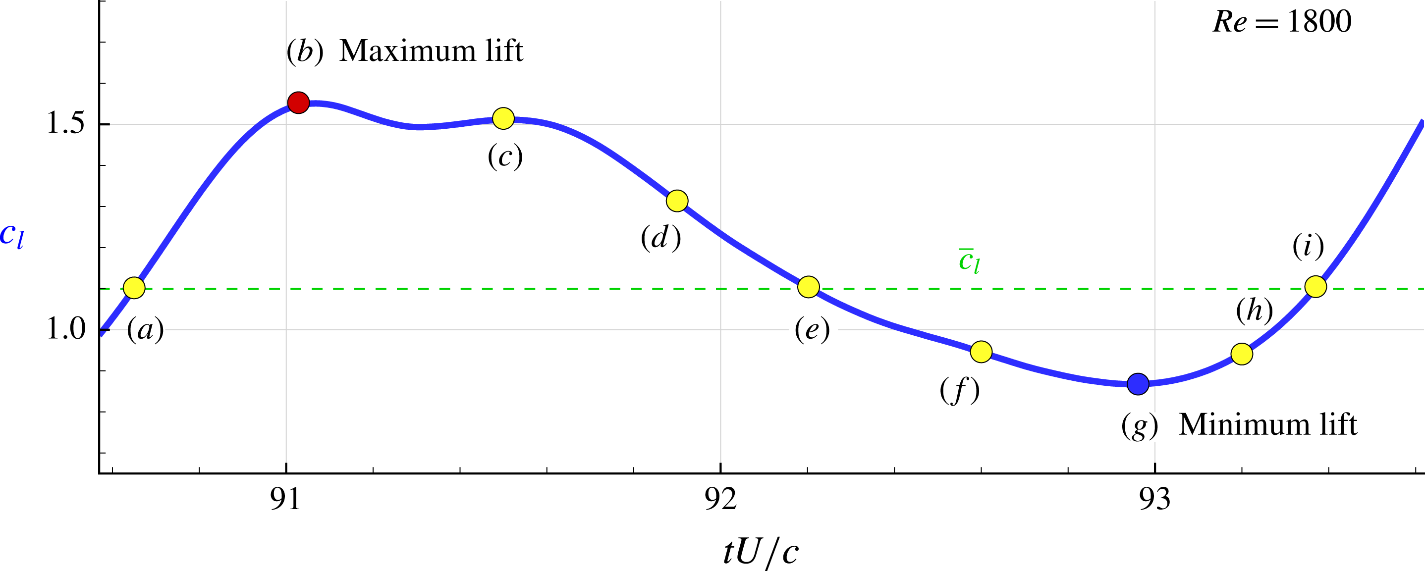
Figure 16 reports an enlarged view in time of the lift evolution for the case
 $U_{2}$
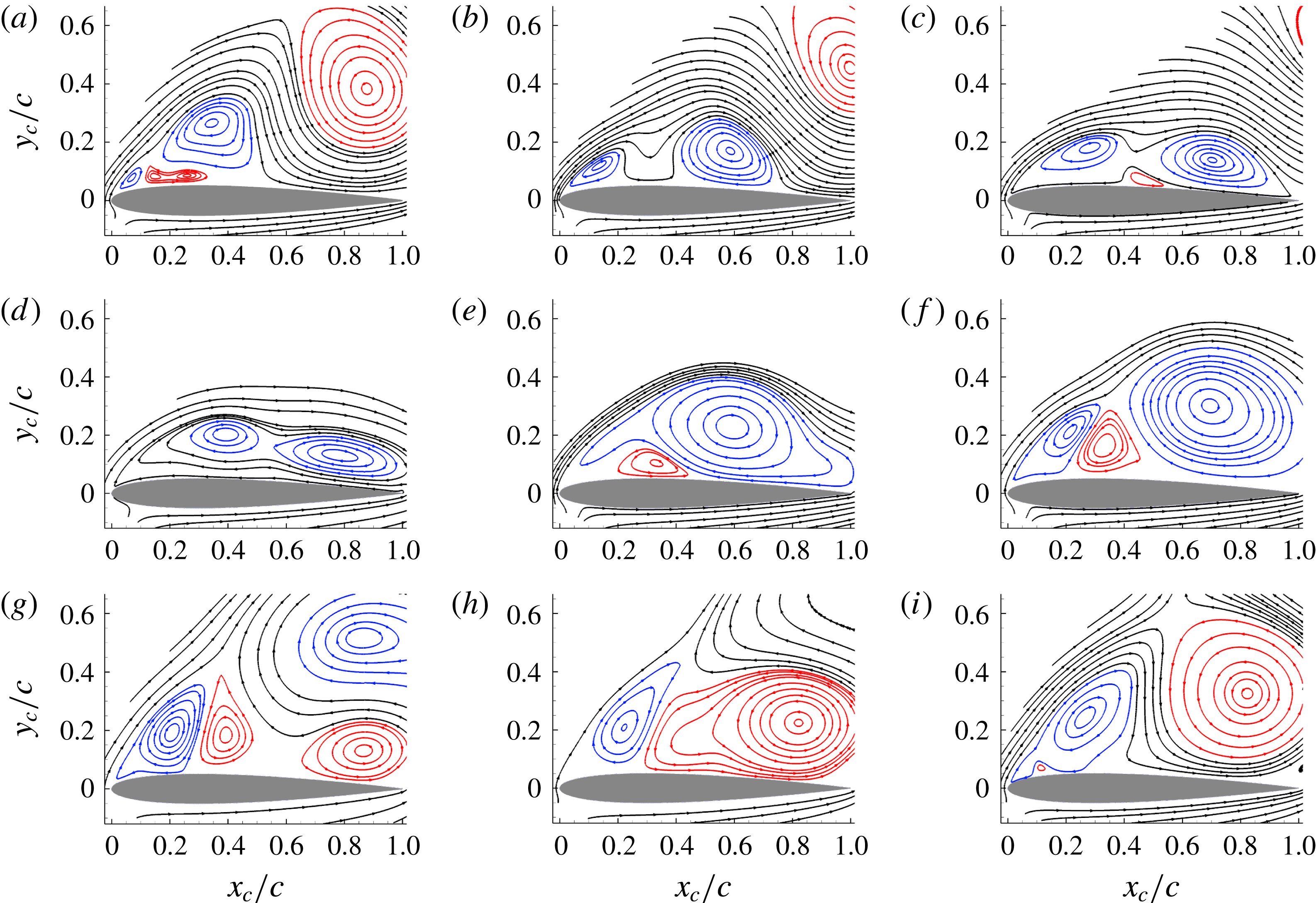
. From this plot it is possible to better see the nonlinear behaviour of the time evolution. Nine different instants have been identified and the streamlines of the velocity fields corresponding to these nine instants are reported in figure 17. For these plots a rotated frame of reference is used and abscissa and ordinate are indicated as
 $x_{c}$
and
 $y_{c}$
, respectively. The streamlines belonging to clockwise and anti-clockwise vortices are depicted with different colours to better highlight the flow dynamics. The separation of the leading-edge shear layer occurs almost at the same position
 $x_{c}=0.017c$
during the whole period.
Case
 $U_{2}$
,
 $Re=1700$
: time history of one period of the lift oscillations. Nine instants are highlighted which correspond to relevant changes in the near-field flow in the vicinity of the suction side of the airfoil.

Streamlines of the instantaneous velocity field in the near body region for the case
 $U_{2}$
(
 $Re=1700$
) for nine different instants (see figure 16).

At the first configuration time, labelled (a), a big anti-clockwise vortex influences the velocity field close to the rear part of the airfoil while the upstream part is under the action of a clockwise vortex and of two small counter-rotating vortices. At the following times (b) and (c) the big anti-clockwise vortex of the rear part moves both up and downstream in the wake. It seems to be pushed away by the streamlines getting round the upstream recirculation zone which are actually oriented towards the upper-right direction. Meanwhile, the two upstream clockwise vortices develop up to merge at instant (d). At instants (e) and (f) this newly formed big clockwise vortex moves downstream the airfoil and is then lifted up and downstream at instant (g), as for the previous big anti-clockwise vortex ejected at time (a,b). These two big vortices ejected upwards, at rather close times (g) and (a,b) of the next period, pair up to form the intense lifted-up dipoles visible in figure 7, characteristic of Mode III. While this big clockwise vortex moves downstream the airfoil at times (e,f), a new dipole of small vortices is formed close to the upstream part of the airfoil. At instant (g), being lifted up the big clockwise vortex leaves the room to the formation of a second anti-clockwise vortex which develops on the rear part of the airfoil prior to merge with the upstream anti-clockwise vortex at instant (h), forming a new big anti-clockwise vortex which goes downstream and upwards at further times (i), (a), (b)... starting a new cycle.
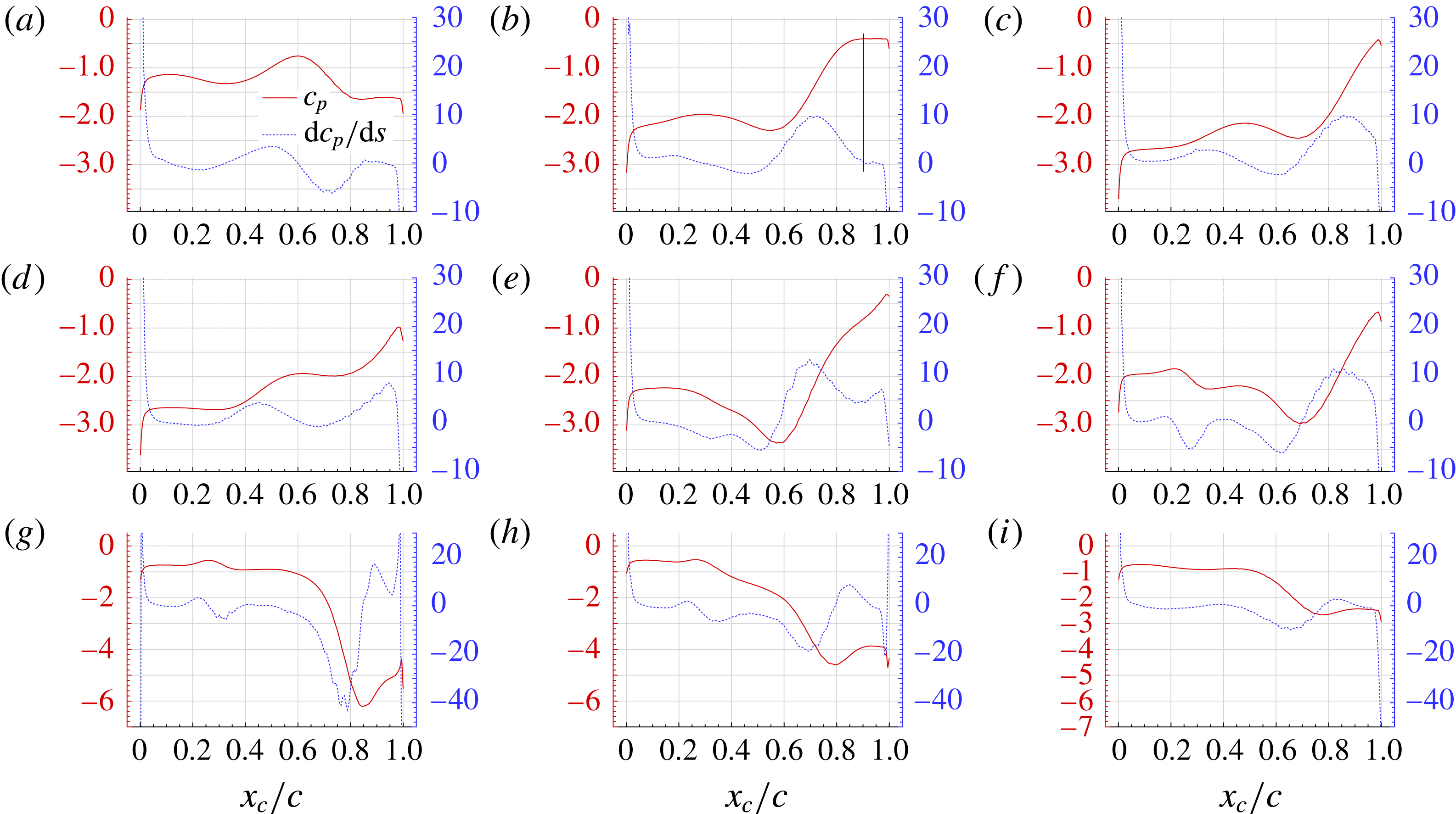
Pressure and spatial derivative of the pressure profiles on the suction side of the airfoil for the case
 $U_{2}$
(
 $Re=1700$
) for nine different instants (see figure 16).

Summarizing, the cycle of Mode III is characterized in the near field by two successive merging of vortices of same sign which form, respectively, a big anti-clockwise and a big clockwise vortex. These two big vortices are ejected upwards and downstream by the incoming flow going round the upstream recirculation zone, giving birth to an intense lifted-up dipole.
In terms of pressure coefficient profiles on the suction side, displayed in figure 18 for the same nine instants, it is visible that the presence of big vortices in the vicinity of the airfoil induces high velocities leading to intense depressions and, in turn, to a more negative mean pressure coefficient than for Mode IV, as shown in figure 15. Conversely, when the flow is partly attached to the profile, the lift force is lower, as for cases (i) and (a) of minimum lift.
From the spatial derivative of the pressure coefficient, it is possible to identify that locations where this derivative is equal to zero actually correspond to stagnation points between the different vortical structures present along the airfoil, as expected and underlined in the analysis by Anand & Sarkar (Reference Anand and Sarkar2017). In their paper they also state that a plateau after a rise in the pressure profile will correspond to reattachment of the boundary layer, which can be verified in plots (b) of figures 17 and 18.
Case
 $L_{2}$
,
 $Re=1800$
: time history of one period of the lift oscillations. Nine instants are highlighted which correspond to relevant changes in the near-field flow in the vicinity of the suction side of the airfoil.

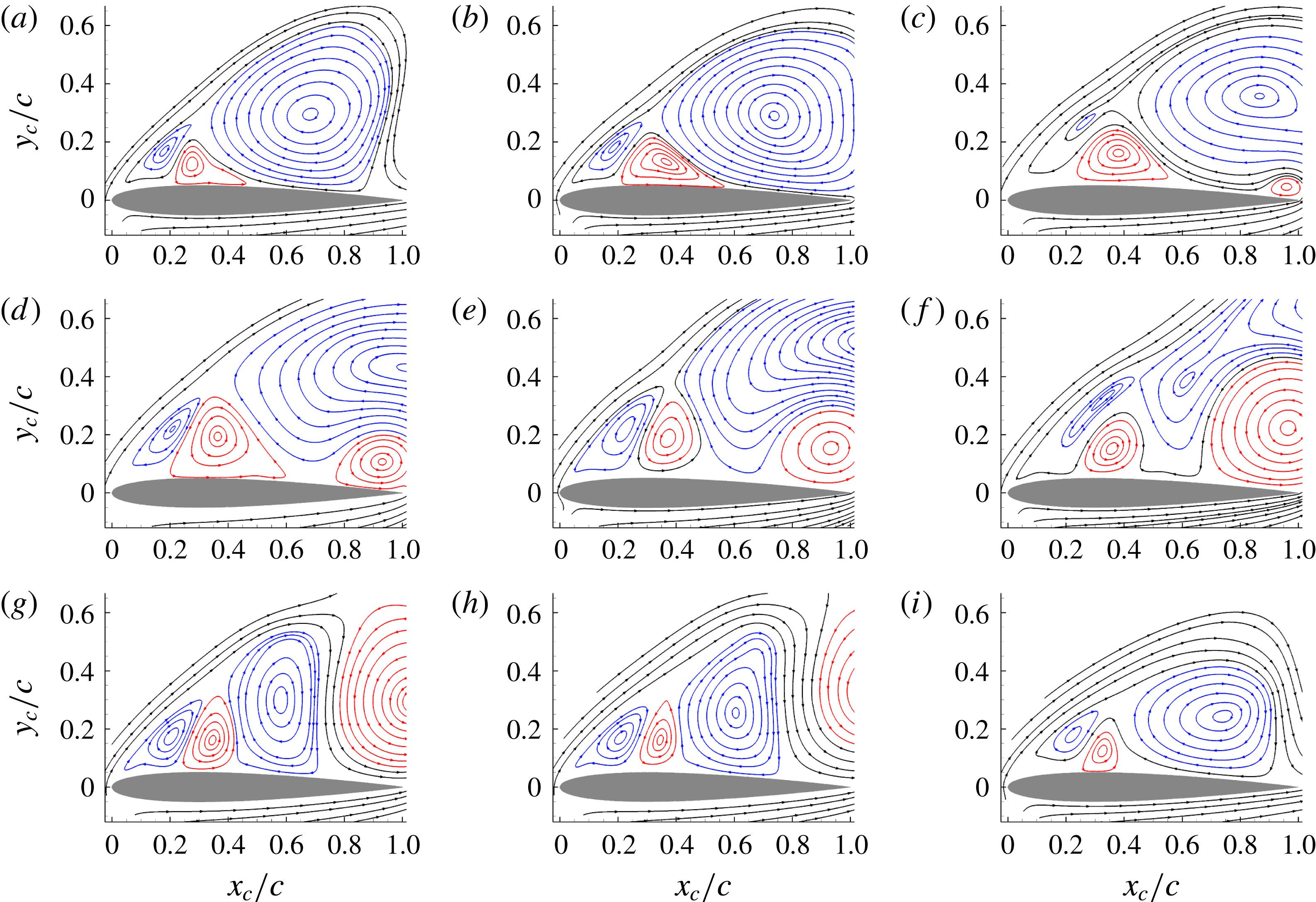
Streamlines of the instantaneous velocity field in the near body region for the case
 $L_{2}$
(
 $Re=1800$
) for nine different instants (see figure 19).

Case
$L_{2}$
– Mode IV

Similarly as for the case
 $U_{2}$
, figure 19 shows an enlarged view of the time evolution of the lift force for the case
 $L_{2}$
(
 $Re=1800$
) characterized by the Mode IV. With respect the case
 $U_{2}$
, the time history presents a more sinusoidal pattern (less nonlinearities). This may be related to the flow dynamics which, this time, does not present vortex merging phenomena. As for the case
 $U_{2}$
nine instants are selected within a period of oscillation and the related streamlines of the velocity fields are reported in figure 20.
A very different sequence can be observed in figure 19 compared to the previous figure 16 for Mode IIIb. The first observation is that, this time, three vortices stay continuously along the airfoil during the whole period: a medium-size clockwise vortex close to the leading edge, followed by an anti-clockwise of approximately same size, followed again by a third vortex, which turns clockwise and whose size evolves during the cycle, contrary to the first two. A second observation which can be made is that the first and third vortices, both turning clockwise, tend to partly merge and split several times during the cycle, especially at instants (c,d) and (f,g).
At instant (a) of the cycle, the large clockwise vortex covers more than half of the chord in the rear part of the profile. This configuration remains relatively stable in time from instants (a) to (c). Progressively, a second anti-clockwise vortex appears close to the trailing edge of the airfoil, at instant (c), and grows continuously up to be ejected downstream at instant (g), not lifted up this time contrary to the Mode IIIb studied above. At the same time, this second anti-clockwise vortex lifts up the downstream part of the large clockwise vortex, at instants (c) to (e), up to splitting it into two parts at instant (f), one part staying along the airfoil between the two anti-clockwise vortices, and one part being released downstream above the second anti-clockwise vortex. The downstream release of the 2 vortices, clockwise and anti-clockwise, occurs almost simultaneously, around instant (g) which corresponds to the minimum lift. The two vortices are thus released downstream in pair, with the clockwise one above the anti-clockwise one, giving birth to dipoles of close to horizontal axis, inducing in turn a compact wake behind the airfoil as can be seen in figure 7.
Summarizing, the cycle of Mode IV is characterized by the presence of 3 ‘permanent’ vortices along the airfoil, with the third one, turning clockwise, which gets bigger and splits into two vortices at each cycle, while the other two almost do not evolve. One part of the split clockwise vortex stays along the profile while the other part pairs with an anti-clockwise vortex which appears, grows and is released close to the trailing edge of the profile. The resulting dipole is thus composed of a clockwise vortex lying above an anti-clockwise one, and thus evolves horizontally behind the airfoil, resulting in a compact wake.
In figure 21, it can be seen that for this Mode IV, the pressure coefficient magnitude is almost constant in the first two thirds of the chord, where lie the 3 ‘permanent’ vortices. This situation does not change during the whole cycle, logically since these vortices do not evolve much along the profile. In addition, the level of depression is less intense compared to Mode IIIb where bigger vortices were present, leading to a lower lift force as for all the cases of the lower branch, see figure 5. However, in the rear part of the chord where the anti-clockwise vortex appears, grows and is released, changes in the pressure coefficient are observed due to this evolution, leading especially to strong depression in this part during the growth of this vortex. This evolution in the rear part of the suction side of the airfoil is responsible for the periodic oscillations of the lift force.
The flow field structures analysed in this section present similarities with the ones studied in Huang et al. (Reference Huang, Wu, Jeng and Chen2001) through experimental visualizations for
 $Re=1200$
and angle of attack equal to
 $30^{\circ }$
. However, in that work the flow field was studied in the transitory regime after a sudden start of the airfoil. Besides, even though similar vortical structures are discussed in Huang et al. (Reference Huang, Wu, Jeng and Chen2001), there is no mention of vortex merging or splitting phenomena which, in our analysis, are important to understand the different flow regimes.
4 Flow around an elliptical airfoil for different Reynolds numbers with angle of attack
$\unicode[STIX]{x1D6FC}=30^{\circ }$

Pressure and spatial derivative of the pressure profiles on the suction side of the airfoil for the case
 $L_{2}$
(
 $Re=1800$
) for nine different instants (see figure 19).

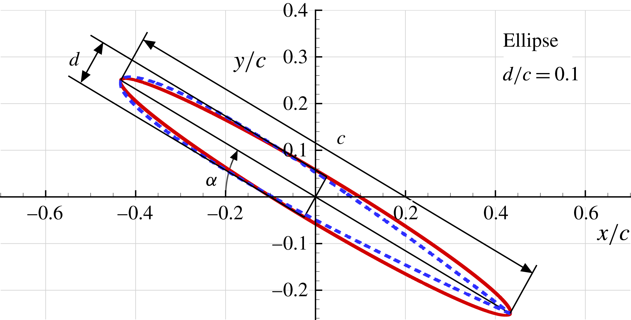
Elliptical profile geometry,
 $c$
and
 $d$
are the major and minor axis, respectively, while
 $\unicode[STIX]{x1D6FC}$
is the angle of attack. Dashed line corresponds to the NACA0010 profile.

Elliptical profile with aspect ratio 0.1,
 $\unicode[STIX]{x1D6FC}=30^{\circ }$
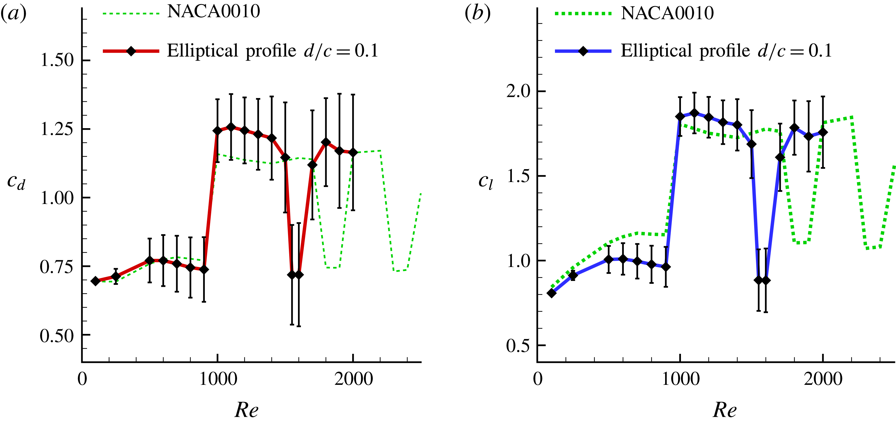
. Mean drag (a) and lift (b) coefficients versus the Reynolds number. Error bars indicate the standard deviation. Dashed lines refer to the mean drag and lift of the NACA0010 profile.

In the present section the flow past an elliptical profile of the same thickness as of the NACA0010 is considered fixing the angle of attack at
 $\unicode[STIX]{x1D6FC}=30^{\circ }$
and changing the Reynolds numbers in the range 100–2000.
Figure 22 presents a sketch of the elliptical profile adopted, which is superimposed to the NACA0010 profile in order to highlight the differences between the two geometries.
In figure 23 the mean drag and lift coefficients,
 $\bar{c}_{d}$
and
 $\bar{c}_{l}$
, and the related standard deviations, are reported together with the ones for the NACA0010 profile. For the studied Reynolds numbers three bifurcations were found: the first between
 $Re=900$
and
 $Re=1000$
, the second between
 $Re=1500$
and
 $Re=1550$
and the third between
 $Re=1600$
and
 $Re=1700$
. Therefore, the first bifurcation is placed at the same Reynolds number as for the NACA0010 while the other ones are anticipated.
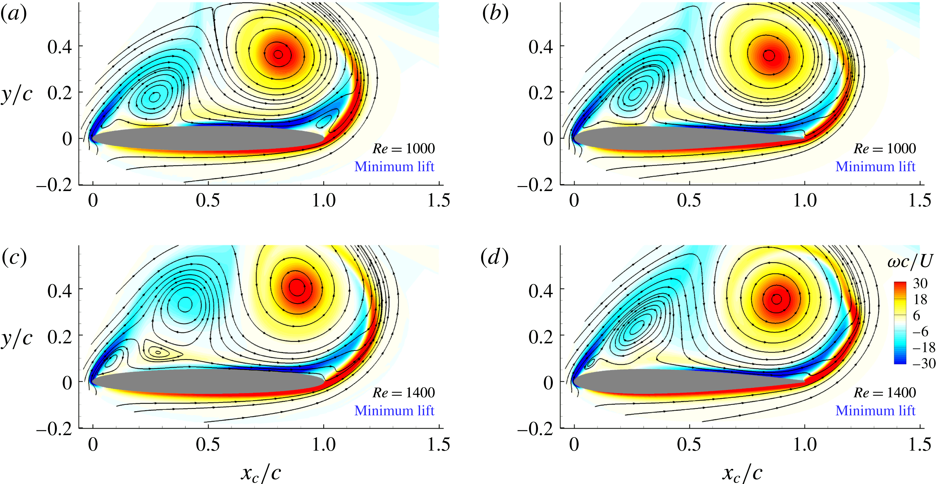
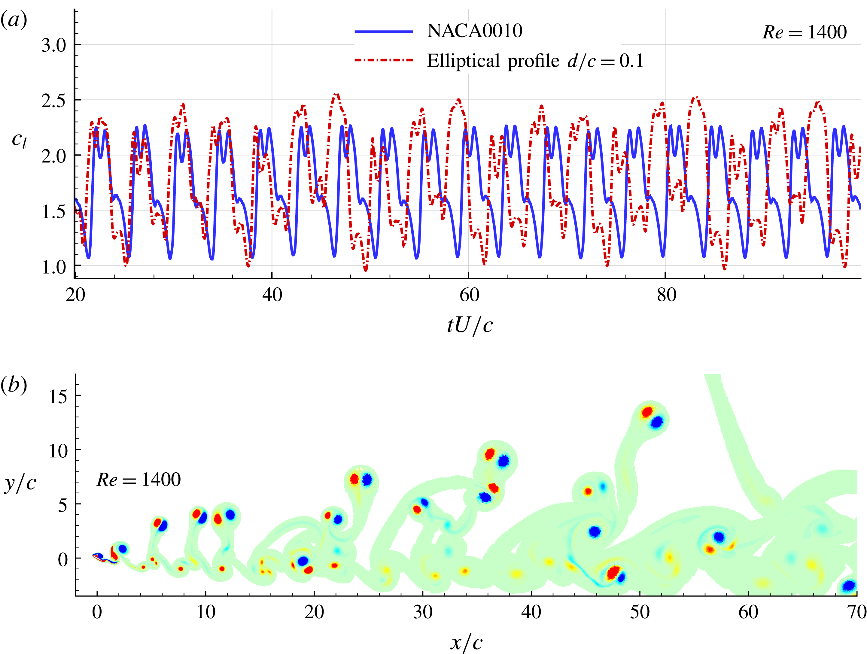
Since the first bifurcation occurs at the same Reynolds number although the shapes of the leading and trailing edges are different, this bifurcation is thus apparently more related to the airfoil thickness than to the local airfoil shape. This can be observed in figure 24 which shows the near-field flow at the minimum lift instant for the ellipse and the NACA0010 airfoils at Reynolds numbers equal to 1000 and 1400. Actually, at
 $Re=1000$
(case
 $U_{1}$
), i.e. close to the first bifurcation, the streamlines and the vorticity patterns for the two profiles are very close even if small local differences are visible. In particular the two big vortices over the suction side look very similar in size and position.
Conversely, for higher
 $Re$
larger differences are present, as can be observed at
 $Re=1400$
in figure 24. Especially, for the elliptical profile the vortices are more distant from the airfoil than for the NACA0010 profile, reducing their influence on the suction side of the airfoil and leaving the room to the formation of smaller structures along the upstream part of the airfoil. As a result the flow around the elliptical airfoil is more unstable, at
 $Re=1400$
, than the flow around the NACA0010 airfoil. Incidentally, the former is characterized by a quite irregular time evolution of the lift (see figure 25
a); those irregularities are also reflected on the wake structure (see figure 25
b). Logically, this difference in stability influences the position of the next bifurcations which occur for lower Reynolds numbers for the more unstable flow, i.e. the one in the near field of the elliptical airfoil, than for the more stable one, i.e. the one in the near field of the NACA0010 airfoil.
Near body vorticity field and streamlines at the minimum lift force instant for the elliptical airfoil (a,c) and the NACA0010 (b,d) for Reynolds numbers
 $Re=1000$
(a,b) and
 $Re=1400$
(c,d). The two airfoils have the same thickness and
 $\unicode[STIX]{x1D6FC}=30^{\circ }$
. Dimensionless vorticity field
 $\unicode[STIX]{x1D714}c/U$
scales from
 $-30$
(blue) to 30 (red).

(a) Time histories of the lift force coefficient
 $c_{l}$
for the NACA0010 and the elliptical airfoil of same thickness at
 $Re=1400$
with
 $\unicode[STIX]{x1D6FC}=30^{\circ }$
. (b) Wake shed by the elliptical profile with
 $\unicode[STIX]{x1D6FC}=30^{\circ }$
at
 $Re=1400$
(non-dimensional time
 $tU/c=100$
, vorticity contour plots range from
 $\unicode[STIX]{x1D714}c/U=-2$
to
 $2$
).

4.1 First bifurcation: case
$L_{1}$
and case
$U_{1}$


For the sake of brevity only the first bifurcation is discussed in this section.
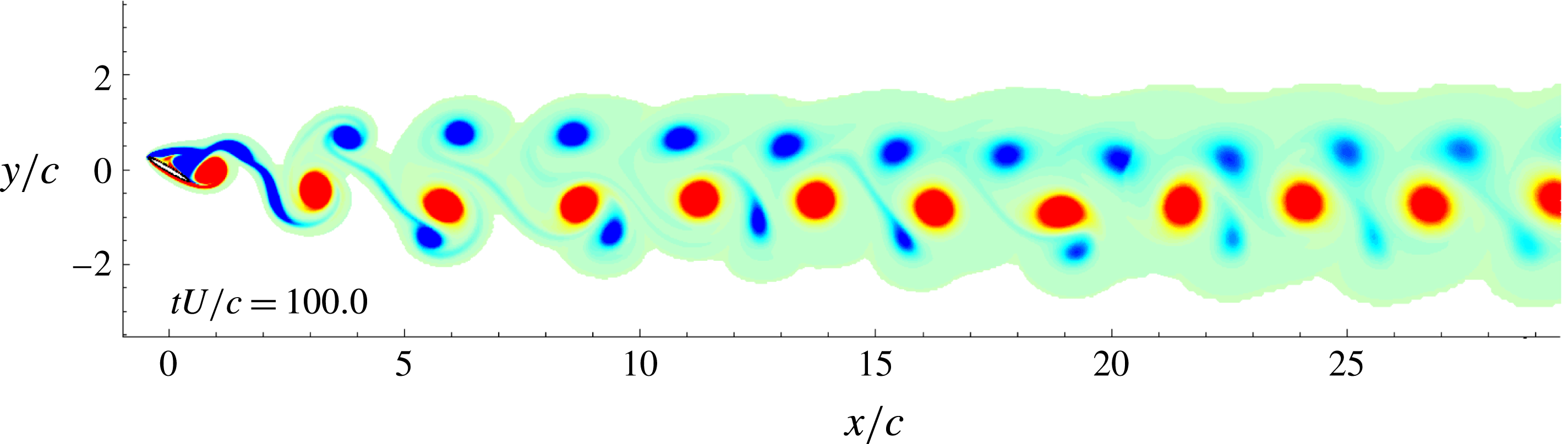
Figure 26 shows the vorticity field for the case
 $L_{1}$
(
 $Re=900$
). Similarly to the NACA0010 results case
 $L_{1}$
is characterized by a Mode IV with a narrow vortex wake confined between
 $y=-3c$
and
 $y=2c$
. With this elliptical profile, differently from case
 $L_{1}$
with the NACA0010, the wake is narrower being the shed vortex structures more intense. The mean lift and drag coefficients are respectively
 $\bar{c}_{l}=0.96$
and
 $\bar{c}_{d}=0.74$
.
At
 $Re=1000$
, as for the NACA0010 (case
 $U_{1}$
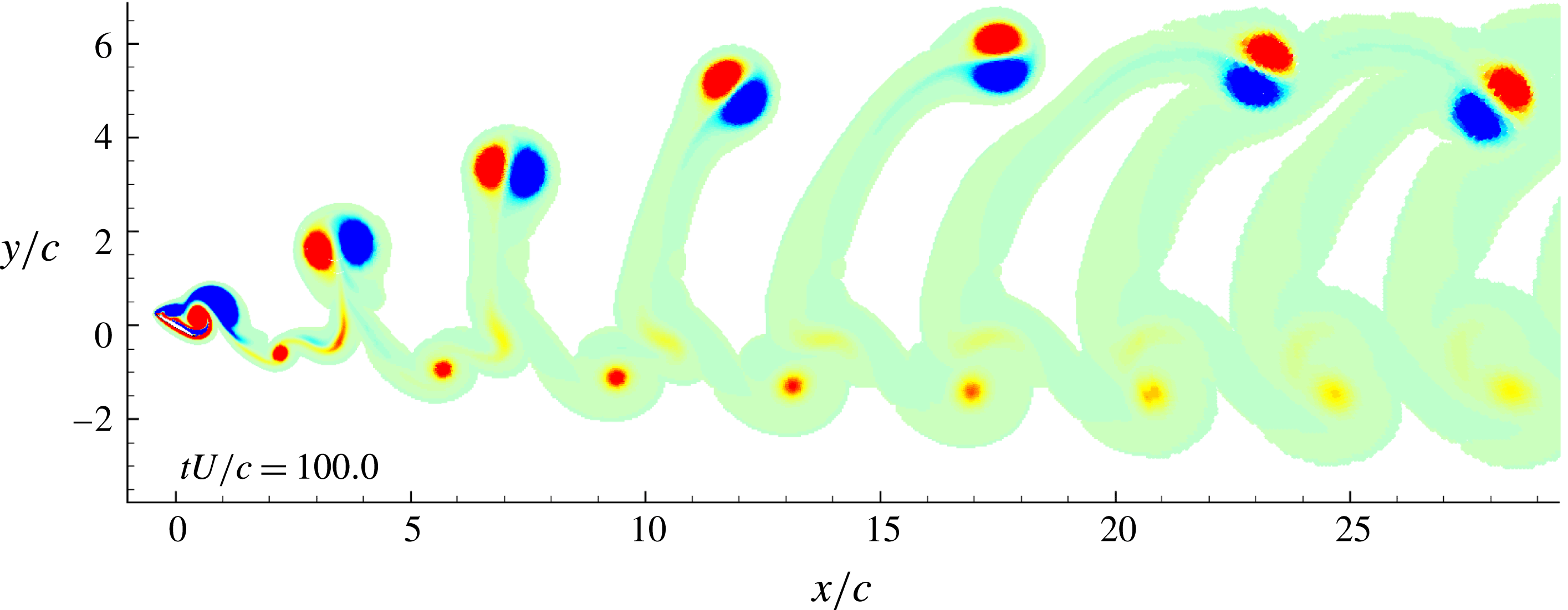
) the flow is characterized by the Mode IIIb (see the vorticity field in figure 27). Due to the bifurcation jump, for the case
 $U_{1}$
the mean lift and drag coefficients have increased values:
 $\bar{c}_{l}=1.85$
and
 $\bar{c}_{d}=1.24$
, respectively. It is worth noting that the jumps of
 $\bar{c}_{l}$
and
 $\bar{c}_{d}$
are more intense than the ones measured for the NACA0010 profile (see figure 23).
The regular shedding behaviour for both cases
 $L_{1}$
and
 $U_{1}$
is reflected on the time evolutions of force components acting on the elliptical profile, as reported in figure 28. It is interesting to note that for
 $Re=900$
the initial part of the time history corresponds to the Mode IIIb. However, this lasts only until
 $t<20\,c/U$
s, after which a bifurcation jump in time appears and the flow reorganizes into Mode IV.
From the frequency analysis (not reported here) the Strouhal numbers are
 $St=0.32$
and
 $St=0.25$
respectively for cases
 $L_{1}$
and
 $U_{1}$
. These values are quite close to the ones evaluated for the NACA0010 profile. Again, as commented in the previous sections, Mode IV presents a shedding mechanism with a fundamental frequency higher than the one related to the Mode III.
Vorticity field for the elliptical profile with aspect ratio 0.1,
 $\unicode[STIX]{x1D6FC}=30^{\circ }$
and Reynolds number equal to 900. The dimensionless vorticity field
 $\unicode[STIX]{x1D714}c/U$
scales from
 $-2$
(blue) to 2 (red).

Vorticity field for the elliptical profile with aspect ratio 0.1,
 $\unicode[STIX]{x1D6FC}=30^{\circ }$
and Reynolds number equal to 1000.

Elliptical profile with aspect ratio 0.1,
 $\unicode[STIX]{x1D6FC}=30^{\circ }$
. Time histories of the drag and lift coefficients for
 $Re=900$
(a) and
 $Re=1000$
(b).

NACA0010,
 $\unicode[STIX]{x1D6FC}=30^{\circ }$
,
 $Re=900$
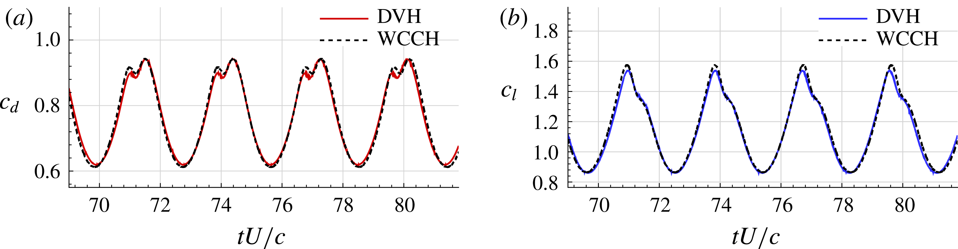
, comparison between the DVH and WCCH methods. (a) Drag coefficient. (b) Lift coefficient.

NACA0010,
 $\unicode[STIX]{x1D6FC}=30^{\circ }$
,
 $Re=1000$
, comparison between the DVH and WCCH methods. (a) Drag coefficient. (b) Lift coefficient.

5 Comparison between DVH and WCCH
In order to investigate how the obtained results are independent from the numerical model used, the DVH results were compared with the WCCH ones at Reynolds numbers
 $Re=900$
and
 $Re=1000$
for the NACA0010 profile.
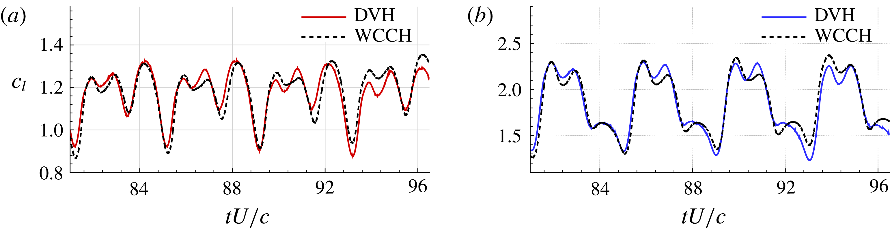
Figures 29 and 30 show the lift and drag coefficient time histories calculated by the two methods. The results are in good agreement, even if some local discrepancies are present especially for
 $Re=1000$
.
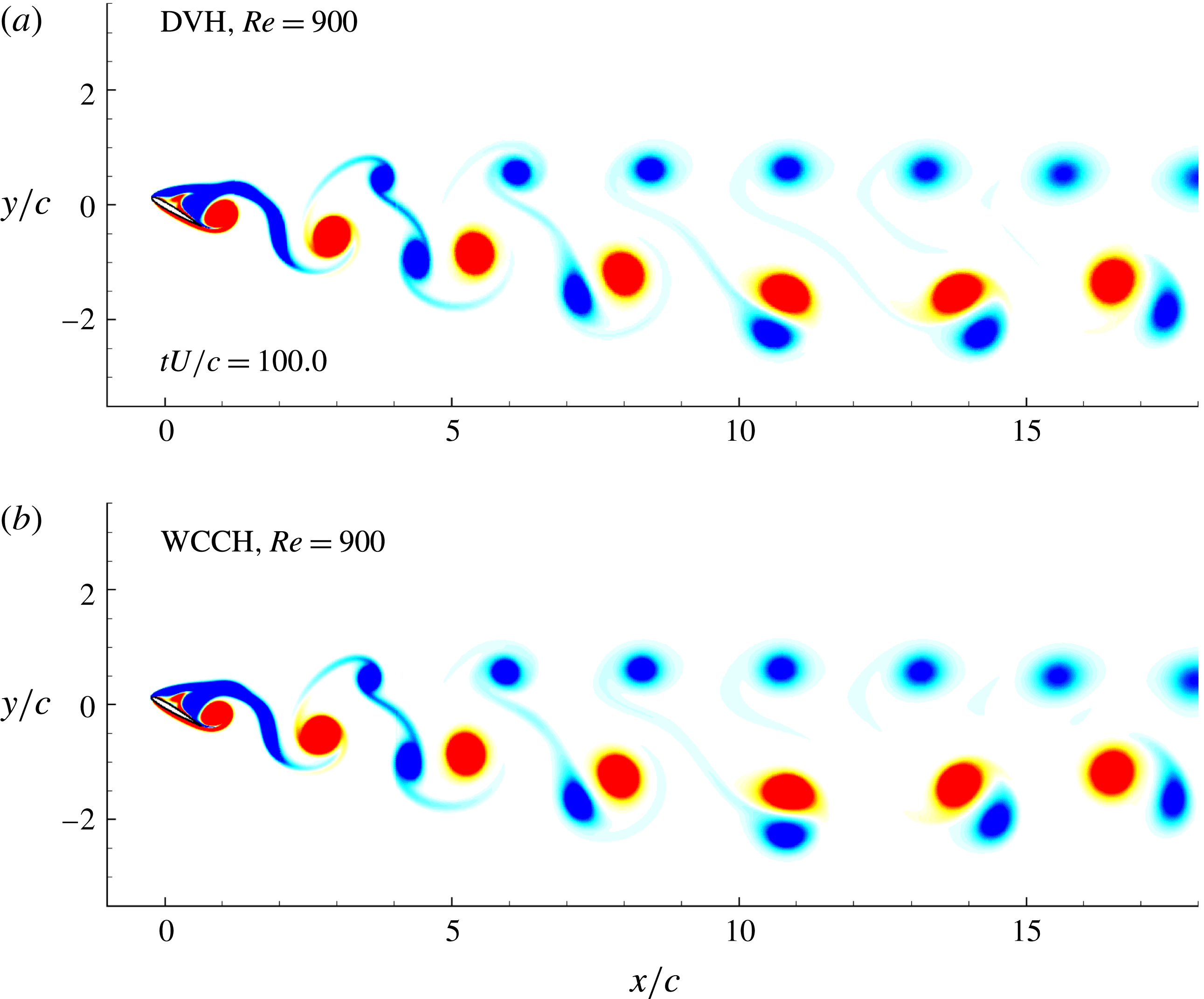
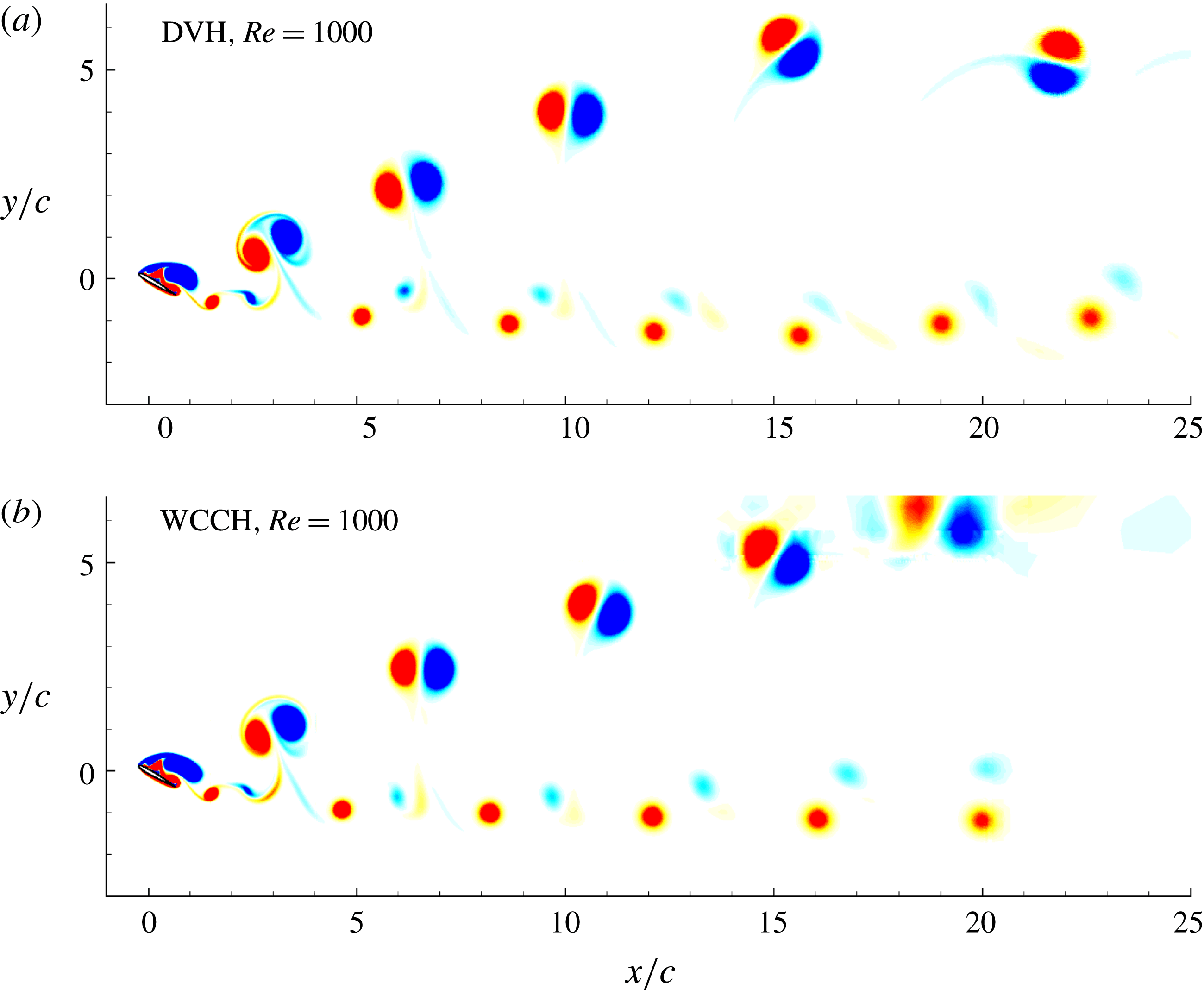
Figures 31 and 32 depict the vorticity fields in the far-wake regions evaluated with the DVH and WCCH methods for the two Reynolds numbers. Both solvers predict a Mode IV vorticity pattern at
 $Re=900$
and a Mode IIIb vorticity pattern at
 $Re=1000$
. The solutions are in fair agreement even if some differences between the solutions are visible in those plots.
Given the very different nature of the two methods, see appendix A, these results are a convincing proof that the DNS results presented and discussed in this article are not sensitive to or dependent on the numerical method chosen.
NACA0010 airfoil,
 $\unicode[STIX]{x1D6FC}=30^{\circ }$
,
 $Re=900$
. Vorticity field with DVH method (a) and with WCCH method (b).

NACA0010 airfoil,
 $\unicode[STIX]{x1D6FC}=30^{\circ }$
,
 $Re=1000$
. Vorticity field with DVH method (a) and with WCCH method (b).

6 Conclusion
The present study is devoted to a numerical investigation of the 2-D flow past a NACA0010 airfoil with angle of attack
 $\unicode[STIX]{x1D6FC}=30^{\circ }$
at different Reynolds numbers, ranging from
 $Re=100$
to
 $Re=3000$
. The analysis highlighted the presence of multiple bifurcations in the flow behaviour which are well detectable in the vorticity field of the wake as well as in the mean lift, drag and pressure coefficients and in the Strouhal number.
The vorticity patterns developed at different Reynolds numbers have been subdivided into five different modes similarly to the analysis performed by Kurtulus (Reference Kurtulus2016), where the flow past NACA0002 and NACA0012 profiles was studied fixing the Reynolds number to 1000 and changing the angle of attack. The bifurcations found in the present work lie in the range
 $Re=900{-}2200$
, where the flow changes multiple times from Mode IV to Mode IIIb and vice versa. These flow pattern changes result in sudden changes back and forth between upper and lower branches in mean lift coefficient, mean drag coefficient and Strouhal number. Careful analysis of the near-field flow close to the suction side of the profile shows that very different mechanisms take place for the 2 modes. For Mode IV, the cycle is characterized by 3 vortices staying permanently along the profile, one of which splits into two parts at each cycle to form a dipole with a fourth vortex growing at each cycle close to the trailing edge. This dipole is ejected downstream with an horizontal trajectory in the wake, leading to a compact wake in thickness. For Mode IIIb, the cycle is characterized by large changes in the vortices present along the profile within each cycle, and especially the merging of, respectively, 2 positive and 2 negative vortices which are lifted up when they are ejected, pairing up in a large dipole which evolves both upwards and downstream, resulting in a typical thick wake with an alley of dipoles raising above the profile position.
Besides the flow over a stalled NACA0010 profile, the flow past an elliptical profile of same chord and thickness has been also studied varying the Reynolds number from
 $Re=100$
to
 $Re=2000$
, with same angle of attack
 $\unicode[STIX]{x1D6FC}=30^{\circ }$
. The results obtained for the two different geometries are very similar, showing that the bifurcations of the solutions are not strictly related to a specific profile shape.
In order to perform the present numerical investigation, a vortex particle method called diffused vortex hydrodynamics (DVH) has been selected, being a method well suited for solving this kind of flows with high accuracy. Particular care is taken in choosing spatial resolutions fine enough to solve all the vorticity length scales present in the field. A cross-validation has also been performed with a second numerical method of very different nature, being based on a finite volume method combined with an immersed-boundary technique and high-order schemes. This method is called weakly compressible Cartesian hydrodynamics (WCCH). Both methods were used for simulating the flow past the NACA0010 airfoil at Reynolds numbers 900 and 1000, where the first bifurcation of the solution was detected. The results obtained are very close to each other, both in terms of local quantities, such as the vorticity field, and global quantities.
Acknowledgements
This work has been supported by CNR-INSEAN and Ecole Centrale Nantes (ECN) within a joint research framework programme. The research activity has been developed within the Project Area ‘Applied Mathematics’ of the Department of Engineering, ICT and Technology for Energy and Transport (DIITET) of the Italian National Research Council (CNR). Authors are thankful to Dr D. Durante for his useful suggestions and interesting discussion on the results obtained in this study.
Supplementary movie
Supplementary movie is available at https://doi.org/10.1017/jfm.2018.189.
Appendix A. Brief description of DVH and WCCH methods
A.1 The DVH method
In this section the diffused vortex hydrodynamics (DVH) method is briefly described. The governing equations adopted in this vortex method are the Navier–Stokes equations written in vorticity
 $\unicode[STIX]{x1D714}$
, which, for a 2-D viscous incompressible flow in the domain
 $\unicode[STIX]{x1D6FA}$
read as:
 $$\begin{eqnarray}\frac{\text{D}}{\text{D}t}\unicode[STIX]{x1D714}=\unicode[STIX]{x1D708}\unicode[STIX]{x0394}\unicode[STIX]{x1D714}\quad \forall \boldsymbol{r}\in \unicode[STIX]{x1D6FA},\end{eqnarray}$$
where
 $\text{D}/\text{D}t$
is the material time derivative and
 $\unicode[STIX]{x1D708}$
is the kinematic viscosity coefficient. In order to solve equation (A 1), an operator splitting scheme (Chorin Reference Chorin1973, Reference Chorin1978) is used for accounting for the vorticity field advection and diffusion. Advection and diffusion are separately considered at each time step. The numerical solution is then obtained by solving an inviscid advective step, governed by the Euler equation:
 $$\begin{eqnarray}\frac{\text{D}}{\text{D}t}\unicode[STIX]{x1D714}(\boldsymbol{r},t)=0\end{eqnarray}$$
followed by a purely diffusive one governed by the heat equation
 $$\begin{eqnarray}\frac{\unicode[STIX]{x2202}}{\unicode[STIX]{x2202}t}\unicode[STIX]{x1D714}(\boldsymbol{r},t)=\unicode[STIX]{x1D708}\unicode[STIX]{x0394}\unicode[STIX]{x1D714}(\boldsymbol{r},t).\end{eqnarray}$$
The presence of a body within the flow field requires an appropriate procedure. Between the advection and the diffusion steps the vorticity is generated on the body contour in order to enforce the no-slip boundary condition.
The vorticity formulation has several advantages: (i) it allows us to discretize only the rotational region of the flow; (ii) the boundary conditions at infinity are automatically satisfied; (iii) the vortex particles are moved in a Lagrangian way.
During the advective step, the velocity field is decomposed in
 $\boldsymbol{u}=\boldsymbol{u}_{\infty }+\boldsymbol{u}_{\unicode[STIX]{x1D714}}+\boldsymbol{u}^{\prime }$
, where
 $\boldsymbol{u}_{\infty }$
is the free stream velocity,
 $\boldsymbol{u}_{\unicode[STIX]{x1D714}}$
is the velocity induced by the vortex particles, while
 $\boldsymbol{u}^{\prime }$
is the contribution to the velocity field due to the presence of the body. The velocity
 $\boldsymbol{u}$
is evaluated using a fast multipole method (FMM) and the vortices are displaced using a fourth-order Runge–Kutta algorithm. From
 $\boldsymbol{u}^{\prime }$
it is also possible to generate a new set of vortices on the body surface, enforcing the no-slip boundary condition exactly on its contour.
The diffusive step is performed following the deterministic algorithm described in Benson et al. (Reference Benson, Bellamy-Knights, Gerrard and Gladwell1989): each vortex particle gives a vorticity contribution on a ‘regular point distribution’ (RPD) by a superposition of elementary solutions of the heat equation. This special set of points will then become the new set of vortex particles substituting the previous one.
Because RPDs are sets of points regularly spaced without any topological connection and the velocity field is evaluated through a FMM, the DVH scheme can be considered as a pure meshless method. The use of RPDs during the diffusion process also prevents the excessive clustering or rarefaction of the vortex particles and avoids remeshing procedures which would be required otherwise (see e.g. Barba, Leonard & Allen Reference Barba, Leonard and Allen2003).
The RPDs around the body are generated using a packing algorithm described in Colagrossi et al. (Reference Colagrossi, Bouscasse, Antuono and Marrone2012), allowing us to arrange points around complex contours, while preserving the volume around each point.
For further details on the DVH method, please refer to Rossi et al. (Reference Rossi, Colagrossi, Bouscasse and Graziani2015a ,Reference Rossi, Colagrossi and Graziani b , Reference Rossi, Colagrossi, Durante and Graziani2016), Colagrossi et al. (Reference Colagrossi, Rossi, Marrone and Le Touzé2016), Durante et al. (Reference Durante, Rossi, Colagrossi and Graziani2016).
A.2 The WCCH method
The weakly compressible Cartesian hydrodynamics (WCCH) method is a finite volume method using Cartesian meshes and a fifth-order weighted essentially non-oscillatory (WENO)-based spatial scheme. The boundary conditions on solid bodies are treated using an immersed-boundary method. The solver uses an adaptive mesh refinement (AMR) algorithm in order to locally increase the spatial resolution. The fluid governing equations used in the WCCH method are the weakly compressible Navier–Stokes equations:
 $$\begin{eqnarray}\left.\begin{array}{@{}c@{}}\displaystyle \frac{\unicode[STIX]{x2202}\unicode[STIX]{x1D70C}}{\unicode[STIX]{x2202}t}+\unicode[STIX]{x1D735}\boldsymbol{\cdot }(\unicode[STIX]{x1D70C}\boldsymbol{u})=0,\\ {\displaystyle \frac{\unicode[STIX]{x2202}(\unicode[STIX]{x1D70C}\boldsymbol{u})}{\unicode[STIX]{x2202}t}}+\unicode[STIX]{x1D735}\boldsymbol{\cdot }(\unicode[STIX]{x1D70C}\boldsymbol{u}\otimes \boldsymbol{u})+\unicode[STIX]{x1D735}P=\unicode[STIX]{x1D735}\boldsymbol{\cdot }\unicode[STIX]{x1D651}+\unicode[STIX]{x1D70C}\boldsymbol{f},\end{array}\right\}\end{eqnarray}$$
where
 $\boldsymbol{f}$
,
 $\unicode[STIX]{x1D70C}$
,
 $P$
,
 $\boldsymbol{u}$
and
 $\unicode[STIX]{x1D651}$
are respectively the body forces, density, pressure, velocity and viscous stress tensor. The problem is therefore decomposed into hyperbolic (Euler equations) and viscous parts. The system is thermodynamically closed with the following equation of state:
 $$\begin{eqnarray}P-P_{0}=c_{0}^{2}(\unicode[STIX]{x1D70C}-\unicode[STIX]{x1D70C}_{0}),\end{eqnarray}$$
where
 $\unicode[STIX]{x1D70C}_{0}$
,
 $P_{0}$
and
 $c_{0}$
are respectively the nominal density, the reference pressure and the nominal speed of sound. This equation of state is barotropic, meaning that no energy equation needs to be solved. Such a formalism is usually encountered in the smoothed particle hydrodynamics (SPH) method (see e.g. Oger et al.
Reference Oger, Marrone, Touzé and de Leffe2016).
For a given cell
 $ijk$
, the Euler equations are finally discretized according to:
 $$\begin{eqnarray}\displaystyle \frac{\text{d}\boldsymbol{W}_{ijk}}{\text{d}t} & = & \displaystyle \frac{1}{\unicode[STIX]{x1D6E5}_{x}}(\boldsymbol{F}_{i-(1/2),j,k}-\boldsymbol{F}_{i+(1/2),j,k})+\frac{1}{\unicode[STIX]{x1D6E5}_{y}}(\boldsymbol{G}_{i,j-(1/2),k}-\boldsymbol{G}_{i,j+(1/2),k})\nonumber\\ \displaystyle & & \displaystyle +\,\frac{1}{\unicode[STIX]{x1D6E5}_{z}}(\boldsymbol{H}_{i,j,k-(1/2)}-\boldsymbol{H}_{i,j,k+(1/2)}),\end{eqnarray}$$
where
 $\boldsymbol{W}=\left(\!\begin{smallmatrix}\unicode[STIX]{x1D70C}\\ \unicode[STIX]{x1D70C}u\\ \unicode[STIX]{x1D70C}v\\ \unicode[STIX]{x1D70C}w\end{smallmatrix}\!\right)$
is the vector of conservative variables, while
 $\boldsymbol{F}(\boldsymbol{W})$
,
 $\boldsymbol{G}(\boldsymbol{W})$
and
 $\boldsymbol{H}(\boldsymbol{W})$
are the flux vectors in directions
 $x$
,
 $y$
and
 $z$
respectively. Finally
 $\unicode[STIX]{x1D6E5}_{x}$
,
 $\unicode[STIX]{x1D6E5}_{y}$
and
 $\unicode[STIX]{x1D6E5}_{z}$
are the cell sizes in the three directions. These fluxes are computed at cell interfaces through the use of a Riemann solver, with left and right states reconstructed spatially using a fifth-order WENO scheme (see for details Liu, Osher & Chan Reference Liu, Osher and Chan1994, Titarev & Toro Reference Titarev and Toro2004). A second-order viscous flux integration method as proposed in Berger, Aftosmis & Allmaras (Reference Berger, Aftosmis and Allmaras2012) is added to the above hyperbolic part. The time integration is performed using a fourth-order Runge–Kutta scheme, for which the explicit nature of the scheme implies the following Courant–Friedrichs–Lewy (CFL) condition:
 $$\begin{eqnarray}\unicode[STIX]{x0394}t=\text{CFL}\frac{\text{min}_{ijk}(\unicode[STIX]{x0394}x_{ijk})}{c_{0}},\end{eqnarray}$$
where the CFL constant is set equal to
 $0.7$
and a fictitious value of
 $c_{0}$
is usually used to obtain larger time steps, always in the limit of the weakly compressible assumption stating that the local Mach number has to remain always and everywhere lower than
 $0.1$
. For further details on the WCCH method the reader can refer to Bigay et al. (Reference Bigay, Oger, Guilcher and Touzé2017).