Introduction

Jakobshavns Isbræ ’ (69 °10′N, 49 °59′W) is the fastest known ice stream, moving more than 7 km a⁻¹ at its calving front (Reference Carbonnel and BauerCarbonnel and Bauer, 1968). It forms at the confluence of two ice streams, a short slow one from the north and a long fast one from the cast. Its last 10 km becomes afloat in Jakobshavns Isfjord on the west coast of Greenland (Fig.1). Figure 1 also shows less concentrated stream flow converging from the southeast. Jakobshavns Isbraæ drains about 6.5% of the Greenland ice sheet (Reference BindschadlerBindschadler, 1984). Our photogrammetric survey was confined to the 10 000 km² area of strongly converging flow into Jakobshavns Isbræ, the area in Figure 1.

Fig. 1.

Uncontrolled photo mosaic map of the Jakobshavns Isbræ: basin. Ice-elevation contours and map-grid tick marks are warped to fit the mosaic. Approximate scale on ice surface is 1: 600000. Contour interval is 100 m. Map coordinates in Figures 1–5 are UTM zone 22 northing and easting in kilometers.

Although its calving front retreated about 27 km from 1850 to 1964, Jakobshavns Isbræ has been close to mass balance equilibrium since then (Reference Pelto, Hughes and BrecherPelto and others, 1989). Rapid retreat has been ascribed to climatic warming at the end of the “Little Ice Age”. At this time surface melting increased considerably, with additional melt water reaching the bed through crevasses and moulins. This enhanced lubrication increased the sliding velocity, which in turn accelerated crevasse formation and iceberg discharge, all in positive feed-back which we call the Jakobshavns effect.

We think that this effect may be migrating northward along the east and west coasts of Greenland in response to the general Holocene climatic warming (Reference HughesHughes, 1986). However, the detailed history of retreat is controlled by fjord topography, especially sharp bends, bottlenecks and pinning points (Reference Warren and HultonWarren and Hulton, 1990). The present surface morphology of Jakobshavns Isbræ reveals that it snakes along a subglacial continuation of Jakobshavns Isfjord that extends into the Greenland ice sheet, displaying all of the above geographical constraints on stream flow (Reference Echelmeyer, Clarke and HarrisonEchelmeyer and others, 1991). These constraints probably account for the stabilization of the calving front and grounding line of the floating terminus since 1964.

The high ablation rates on the floating terminus and on ice converging on Jakobshavns Isbræ: produce surface meltwater which enters crevasses and moulins to either refreeze internally or lubricate the bed. therein sustaining the rapid flow (Reference Echelmeyer and HarrisonEchelmeyer and Harrison, 1990; Reference Echelmeyer, Clarke and HarrisonEchelmeyer and others. 1991, Reference Echelmeyer, Harrison, Clarke and Benson1992), as required for the Jakobshavns effect.

Photogrammetry

The University of Maine carried out a project in 1985 and 1986 to obtain ice-surface elevations and summer and annual velocities for the Jakobshavns Isbræ basin by aerial photogrammetry and to produce orthophotos maps of the area. The orthophotos and elevation-contour overlayas were produced as 14 sheets at 1:50 000 scale.

In order to detect any differences between summer and annual velocities, two photo missions, a year apart and each conducted twice in the same summer, ideally at least 3 weeks apart, were specified. The measurements 1 year apart were designed to maximize the accuracy of velocity determination for the slower ice converging on the main ice stream, whereas the two measurements in the same summer were designed to maximize the accuracy of the velocities for the much faster ice in Jakobshavns Isbræ itself. Photography at a scale of 1: 130 000 yields ground resolution and measurement precision of about 2 m. Positions and elevations were to be determined by analytical aerial-block triangulation for each epoch. Targeted control points spaced two to three photo-base lengths apart along the perimeter with two additional points in the interior of the block were planned. Their positions were to be determined by Doppler satellite surveys.

Mainly due to weather limitations, the photo missions were actually flown 2 weeks apart in July in both 1985 and 1986, which reduced the accuracy of the summer velocity determinations because position errors are a larger fraction of the motion over this shortened time interval. The actual scale of the photographs in both seasons was somewhat smaller than specified, but this did not seriously affect the precision of the measurements. More than the minimum desired number of targets were set out and usable in each season and, with one or two exceptions, the desired precision of their ground positions was attained. However, difficulties with navigation, satellite-receiver malfunctions and loss of targets from wind or burial by blowing snow resulted in less than optimal distribution of ground-control points and thus in some degradation of the block-triangulation results.

No unequivocal figures for accuracy of position determinations, and thus velocities, can be given because no check points are available. Standard deviations of ground coordinates from the aerial triangulation-block adjustment, which come from error propagation of photo and ground-control point residuals, are given in Table 1. Standard deviations of motions calculated from the position errors of Table 1 and relative errors for the three representative extremes of motion are given in Table 2. Precision Statistics are often overly optimistic, but it should also be noted that a number of points in each epoch were discarded because they were adjudged to give unreasonable motion results. It can be argued that these were probably the most poorly determined points. Thus the statistics displayed in the tables may not be an unreasonable indicator of the accuracy of the accepted results.

Table 1.

Standard deviations of ground coordinates from aerial triangulation-block adjustment

Table 2.

Standard deviations of motions

The number of accepted points for each epoch and the number of common points for each velocity determination are summarized in Table 3. The four combinations for the “year” 1985 8G yielded 338, 395, 333 and 408 acceptable common points.

Table 3.

Number of accepted points for each epoch and number of common points for each velocity determination

Within the accuracy of our measurements, we found no difference between annual and summer velocities, thereby confirming the measurements by Reference Echelmeyer and HarrisonEchelmeyer and Harrison (1990). In our further analysis of ice dynamics presented here, however, we have used only the points measured in 1985 because there are more of them and their distribution is more representative both of regional ice converging on the main ice stream and of Jakobshavns Isbræ itself than is the case for any other time interval.

Figure 2 locates the points measured on 10 July 1985 and gives the elevation for each point. Figure 3 is the icc-surface-elevation contour map based on these points. Figure 1 shows velocity vectors originating at the first position of the common points from which the velocity was determined. Figure 5 is the Ice-surface-speed contour map based on these velocities. The gridding and contouring were performed with the SURFACE II plotting package Reference SampsonSampson, (1978).

Fig. 2.

Locations and elevations (m) of ice-surface points measured photogrammetrically for the Jakobshavns Isbræ basin on 10 July 1985 photography.

Fig. 3.

Ice-surface-elevation contours derived from points in Figure 2 by gridding at 3 km intervals using the SURFACE II plotting package. Contour interval is 20 m.

Fig. 5.

Ice-speed contours derived from velocity vectors in Figure 4 by gridding at 3 km intervals using the SURFACE II plotting package. Contour interval is 50 ma⁻¹.

Interpolation and Derivatives

Using our photogrammetrically determined surface-ice topography and velocity measurements, we have calculated surface strain rates, surface stresses and bed topography for an area of about 100 km on each side.

The raw data are irregularly spaced due to their dependence on identifiable natural features. To facilitate analysis, a regular grid with a 3 km spacing spanning a 100 km by 100 km area surrounding the Jakobshavns Isbræ outlet glacier was developed from the raw data using the SURFACE II plotting package. This spacing closely approximates the spacing of the observed natural features but provides the data in an easier-to-manipulate format.

From these elevation data we can derive surface slopes based on two-dimensional bilinear interpolation. Treating each quadrangle of gridded-surface elevations, or nodes, as an element, we may interpolate any quantity specified at the four corners by the following expression:

where the Z_Is are the values of the interpolated quantity at each of the four nodes, and the 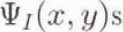are bilinear basis functions with the specified property that each be 1 at one node and 0 at all the other nodes. It is easy to see that spatial derivatives of nodal quantities can be obtained from Equation (1). Since only the 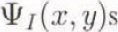depend on horizontal rectilinear axes x and y, we obtain the following expressions for the derivatives of nodal-point quantities:

This treatment is not restricted to “square” quadrilaterals and can be used on any arbitrarily shaped element. The magnitude of the surface gradient, , is given by

where and are obtained from Equations (2) and (3), Figure 6 shows a contour plot of this surface gradient obtained from the gridded data.

Fig. 6.

Surface-elevation gradient contours derived from the gridded data in Figure 3.

Strain Rates and Stresses

Using the interpolation machinery described above we can derive strain rates for each clement. To make interpretation easier, we shall look at the strain rates for each element aligned longitudinally (L) and transversely (T) with respect to the direction of flow at the centroid of the element, rather that with respect to the X and Y axes. To do this we must first obtain the direction of flow at the centroid. The velocities at each node are decomposed into X and Y components, and using an expression similar to Equation (1) we can obtain velocity components at the centroid. These will represent the “average” or interpolated flow for the element. The angle of the L axis relative to the X axis is given by the following expression:

Each of the nodal-velocity values can then be transformed to the “average” flow direction by the following expressions:

Gradients of these L and Τ components of the velocities with respect to X and Y can be obtained using interpolation expressions similar to Equations (2) and (3).

Finally, gradients along the L and Τ directions can be obtained with expressions analogous to Equations (6) and (7).

Surface strain rates with respect to these local flow directions are given as usual by the following expressions and are shown in Figure 7a–d:

where Equation (19) expresses conservation of ice volume.

Fig. 7.

a. Contours of surface longitudinal strain rate 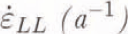along ice flow. b. Contours of surface transverse strain rate 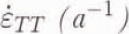across ice flow. c. Contours of surface shear strain rate 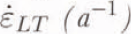with respect to ice-flow direction, d. Contours of surface vertical strain rate .

The surface stress field can be calculated from the surface strain rates in Equations (16)–(19) using the flow law of ice (Reference NyeNye, 1952) written in terms of the effective creep rate and the effective creep stress :

and in terms of Strain-rate components and deviatoric-stress component :

where A is a temperature-dependent ice-hardness parameter, n is a visco-plastic parameter, and ij is LL, TT or LT.

Combining Equations (20) and (21), and solving for 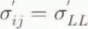we have:

By definition, with as a free-surface boundary condition, we have:

where for conservation of volume, and by definition:

An expression for σ_c in terms of RLL and σ′_LL is obtained from Equations (20)–(22) for ij = LL:

Surface stresses can now be expressed in terms of measured surface strain rates using Equation (21) with ij being LL, TT and LT, and n = 3 for glacial ice:

and A can be calculated from the mean annual ice-surface temperature (Reference GlenGlen, 1955). Stresses with respect to the L and Τ directions obtained from Equations (28)–(30) are shown in Figure 8a–c.

Fig. 8.

a. Contours of surface longitudinal deviatoric stress σ′_LL (bar) along ice flow. b. Contours of surface transverse deviatoric stress σ′_TT (bar) across ice flow. c. Contours of surface shear deviatoric stress σ′_LT (bar) with respect to ice-flow direction.

Derived Bed Topography

With the extensive photogrammetric measurements on Jakobshavn Isbræ and its catchment area, we are able to treat the measured surface elevations and velocities as known quantities, and derive the ice thickness necessary to produce this flow within the constraints of a particular value for the flow constant, the sliding constant and the fraction of the velocity which is due to sliding.

The column-averaged flow velocity obtained from Equation (21) for the component of velocity due to internal deformation of the ice is given by the following expression:

where A is the column-averaged How constant for an ice column of thickness Η and of surface height h above sea level, ρ is ice density and g is the acceleration of gravity.

The sliding law used here is a general relationship for beds at the melting point developed by (Reference WeertmanWeertman 1957, Reference Weertman1964) and given by the following expression:

where parameter Β includes bed roughness and m is a visco-plastic parameter for sliding temperate basal ice. We use this sliding law because it applies to rough bedrock, not to a deformable till. The deglaciated area beyond the ice margin is nearly all exposed bedrock, with little or no till cover (see Fig.1).

The column-averaged ice velocity for a combination of these two modes of motion is

where f is the fraction of velocity due to sliding. What f dose is reduce the vertical shear gradient in ice as basal sliding replaces internal shear in contributing to total ice velocity. Without f, column-averaged values of A and constant Β in Equations (31) and (32) would have to be replaced with values of A and Β that depended on what fraction of the bed allows basal sliding. There is no physical reason for A and Β to depend on this fraction, although f itself most likely depends on the basal temperature, which is not calculated in this model. Others have attempted to calculate basal temperatures for fast-flowing ice by explicitly including horizontal advection (Reference Funk, Echelmeyer and lkenFunk and others, 1993), but accurate calculation of basal temperatures will probably require a full three-dimensional temperature solution.

Combining Equations (31), (32) and (33), one obtains the following expression relating the measured velocity fields and surface elevations to the unknown ice thicknesses:

where the flow and sliding exponents, n and m have been replaced with their traditional values, 3 and 2, and A and Β are taken to be 3.0 bar ma and 0.03 bar ma, respectively. This presents a fourth-degree equation in H, the ice thickness, which can be solved by ordinary numerical methods. Strictly speaking, both U and are themselves vector quantities, so that two equations relating the X and Y components of the velocity with the X and Y Surface gradients are available. We have chosen to relate the magnitude of the velocity to the magnitude of the surface gradient to avoid ambiguities due to inaccuracies in the measured data. When a thickness has been obtained, the bedrock elevation can be obtained by simply subtracting the thickness from the measured surface elevation, (see Fig.9).

Fig. 9.

Calculated bedrock-elevation contours (m).

The accuracy of this calculated bedrock surface is dependent upon the accuracy of the original measured surface-elevation and velocity data, as well as upon the values chosen for the various constants, A, the flow-law parameter, B, the sliding-law parameter, and f, the percentage of the velocity due to sliding. Reference Bahr, Pfeffer and MeierBahr and others (1992) have shown that small errors in measured surface strain rates alone lead to large errors in calculated ice thicknesses. Their prediction can be tested by comparing our calculated ice thicknesses with those measured by K. Echelmeyer (unpublished information). To understand the sensitivity of the calculated bed’s dependence on these inputs, we varied the data and parameters systematically and observed the change in the average thickness, from which the bed is directly calculated. We observed that the greatest variation in average thickness occurred for variation of the measured surface height, a decrease of 14.8 m for each 1% overestimate of the surface height. The next strongest was the sliding constant, B, for which an increase of 8.9 m for each 1% overestimate of the constant was observed. An overestimate of the measured velocity by 1% resulted in an increase in thickness of 6.4 m. An overestimate of the flow constant by 1% resulted in an increase in thickness of 5.8 m. Least sensitive was the dependence of the thickness on the choice of the fraction of the velocity due to sliding, which indicated a decrease in the surface elevation of only 4.2 m for each 1% overestimate in the fraction. Unfortunately this is the least well-constrained of the input parameters, and an overall variation for the entire range of allowed fractions (0 for no sliding, 1 for all sliding) is over 1600 m. These results are summarized in Table 4.

Table 4.

Change in average thickness for 1% overestimate

Assuming an error in all estimated parameters and measured data of 10%, the thickness would be in error by about 400 out of 1600 m, or about 25%. It is clear that this derived bed is an estimate of the underlying terrain, and not a rigorous measurement.

This bedrock surface is used as input to the map-plane finite-element model, from which a calculated surface is obtained. The finite-element model is a column-averaged continuity-equation solver described in detail elsewhere (Reference Fastook and PrenticeFastook and Prentice, 1994). Briefly this model solves a two-dimensional continuity equation

where σ is the flux through a point, is the net mass balance at a point, and h is the ice-surface elevation. A differential equation is obtained by expressing the flux as

Where U is the column-averaged velocity of Equation (34) and H is the ice thickness. The non-linear constant k(x, y) incorporates the physics of the flow and sliding laws into the problem, since its form depends on the form of the flow and sliding laws. Different treatments of the flow and sliding processes change the form of k(x, y) but do not affect the method by which the problem is solved. The resulting non-linear differential equation

can be solved by an iterative Galerkin finite-element formulation (Reference Becker, Carey and OdenBecker and others, 1981).

In this model the fraction of the velocity due to sliding has been used as an adjustable parameter to obtain a good fit to the measured surface. This is done in an iterative fashion where the surface at each node is compared with the measured surface, and a correction to the fitting parameter applied in such a way as to improve the fit. After approximately 1000 iterations the distribution-of-sliding fraction shown in Figure 10 is obtained. Note the predominance of sheet flow over most of the region, with sliding-dominated flow occurring just before the ice stream becomes afloat. Minor branches of enhanced-sliding regions extend out along the primary branch of the ice stream (flow from the east), although there is no evidence in the fitted fraction for the secondary branches of the ice stream (flow from the north and from the southeast).

Fig. 10.

Fraction of total ice velocity due to basal sliding.

One must certainly note that the procedure for estimating the bed topography itself uses the fraction f and that this fraction is then fitted using the finite-element model. Attempts to iterate this process were unsuccessful. Instead a small fraction (0.10) is used in the bed generation process, and the finite-element model can be considered to be a means of refining the detail in the spatial distribution of sliding.

The surface calculated from this sliding-fraction distribution is shown in Figure 11, and the agreement with the measured surface is quite good. Some of the finer details of the surface are lost in this calculation, but this is to be expected considering the limitations of the column averaged model.

Fig. 11.

Calculated surface-elevation contours, indicated by solid lines, and measured surface elevation contours, indicated by dashed lines.

In addition to calculating the surface, the map plane finite-element model also provides velocities, which are shown in Figure 12. In general there is quite-good agreement with the general pattern derived from measured velocities seen in Figures 4 and 5. The three branches of the ice stream are still evident, although the separation is not as clear. There are minor discrepancies north of the ice stream where the measured west-to-east flow is not duplicated in the calculated velocities, and the complex flow pattern measured in the southwest quadrant is also not manifest in the calculated velocities.

Fig. 12.

Calculated surface velocity vectors (m a⁻¹) for comparison with measured vectors in Figure 4.

Fig. 4.

Ice-velocity vectors from point positions determined photogrammetrically on 10 and 24 July 1985 photography.

This paper demonstrates the possibility of deriving an approximation of the bedrock topography underlying an area with sufficient repeated photogrammetric coverage to obtain surface velocities and elevations. This technique can be used when radar flight-line coverage is insufficient or unavailable. While the steps in this exercise are somewhat circular (we have used a column-averaged velocity to obtain the thickness, which we then modeled with a column-average model), we are provided with initial conditions for further work on the catchment area, which can include modeling of the behavior of the grounding line in response to changing climatic conditions. In a sense, what we have done is “tune” our model, in a manner analogous to the “tuning” that is done on global circulation models. Further tests of the model’s behavior in the time domain will help us to refine and validate these assumptions.