1. Introduction and background
Wall-bounded turbulence governs a variety of flow processes (e.g. mixing, heat and mass transfer) and is key to the aerodynamic and hydrodynamic performance of most engineering systems (Marusic, Mathis & Hutchins Reference Marusic, Mathis and Hutchins2010). To understand the behaviour of these seemingly chaotic flows, researchers have traditionally focused on the smooth-wall boundary-layer problem, particularly on the structure of organised motion and the inter-scale dynamics that occur very close to the surface. Numerous experimental and numerical studies have shown that the logarithmic and outer regions are populated by streamwise-elongated coherent structures, which carry a significant fraction of the turbulent kinetic energy and Reynolds shear stress (Ganapathisubramani, Longmire & Marusic Reference Ganapathisubramani, Longmire and Marusic2003; Tomkins & Adrian Reference Tomkins and Adrian2003; Hutchins & Marusic Reference Hutchins and Marusic2007a). These distinct features scale with the thickness of the boundary layer  $\delta$ and exhibit a spanwise meandering motion. Despite controversy, it is generally accepted that they are a result of an assemblage of hairpin-type vortices, termed vortex packets, whose interaction at different scales determines the turbulent properties of the boundary layer (Kim & Adrian Reference Kim and Adrian1999; Christensen & Adrian Reference Christensen and Adrian2001; Marusic Reference Marusic2001; Ganapathisubramani et al. Reference Ganapathisubramani, Longmire and Marusic2003; Hambleton, Hutchins & Marusic Reference Hambleton, Hutchins and Marusic2006). They have been found to leave a footprint onto the near-wall turbulence (Metzger & Klewicki Reference Metzger and Klewicki2001; Abe, Kawamura & Choi Reference Abe, Kawamura and Choi2004; Hoyas & Jiménez Reference Hoyas and Jiménez2006) and to modulate the amplitude and frequency of the small scales (Hutchins & Marusic Reference Hutchins and Marusic2007b; Mathis, Hutchins & Marusic Reference Mathis, Hutchins and Marusic2009; Ganapathisubramani et al. Reference Ganapathisubramani, Hutchins, Monty, Chung and Marusic2012; Baars, Hutchins & Marusic Reference Baars, Hutchins and Marusic2016). They additionally have direct implications for the local fluctuations of wall shear stress. Hutchins et al. (Reference Hutchins, Monty, Ganapathisubramani, Ng and Marusic2011) showed, by conditional averaging the flow field with data from surface probes, that a negative skin-friction event is more likely to occur in the presence of a low-speed, large-scale motion (LSM). This is usually accompanied by an attenuation of the small-scale energy near the wall and amplification in the outer region (the behaviour is reversed for large-scale positive fluctuations). Scale interactions become increasingly prominent with the Reynolds number
 $Re_{\tau }$, as the spectral separation increases and the large-scale, outer-layer events become more energetic (De Graaff & Eaton Reference De Graaff and Eaton2000; Metzger & Klewicki Reference Metzger and Klewicki2001). This leads not only to an increase of the near-wall turbulence intensity via superposition of energy by the large scales, but also to an increase of the amplitude modulation (AM) (Mathis et al. Reference Mathis, Hutchins and Marusic2009).
Rough-wall-bounded turbulence has also received considerable attention. Within the roughness-affected layer, the influence of the roughness elements causes the flow to be spatially inhomogeneous and creates intense shear and intermittent sweep and ejection motions. Depending on the roughness Reynolds number and the surface geometry, these events may potentially disturb the turbulence structure of the entire boundary layer (Krogstad, Antonia & Browne Reference Krogstad, Antonia and Browne1992; Bhaganagar, Kim & Coleman Reference Bhaganagar, Kim and Coleman2004; Placidi & Ganapathisubramani Reference Placidi and Ganapathisubramani2018). Otherwise, if the roughness sublayer does not extend far from the wall, they only modify the boundary conditions for the outer flow, leaving its structure qualitatively unchanged (Perry & Abell Reference Perry and Abell1977; Flack, Schultz & Shapiro Reference Flack, Schultz and Shapiro2005; Volino, Schultz & Flack Reference Volino, Schultz and Flack2007). Rough-wall boundary layers then show important similarities to the smooth-wall counterpart in terms of shape and scaling of the turbulent features, as well as in terms of inter-scale dynamics. Similar LSMs and vortical structures have been identified (Grass, Stuart & Mansour-Tehrani Reference Grass, Stuart and Mansour-Tehrani1991; Djenidi, Elavarasan & Antonia Reference Djenidi, Elavarasan and Antonia1999; Leonardi et al. Reference Leonardi, Orlandi, Djenidi and Antonia2004; Coceal et al. Reference Coceal, Dobre, Thomas and Belcher2007; Lee, Sung & Krogstad Reference Lee, Sung and Krogstad2011; Lee et al. Reference Lee, Seena, Lee and Sung2012; Mejia-Alvarez, Wu & Christensen Reference Mejia-Alvarez, Wu and Christensen2014). Their spatial coherence is typically reduced in the streamwise direction but increased along the span, and the viscous-normalised spacing between them appears to remain the same. The inner–outer scale interactions have also been documented for many different surfaces, including large two-dimensional ribs (Nadeem et al. Reference Nadeem, Lee, Lee and Sung2015; Blackman, Perret & Savory Reference Blackman, Perret and Savory2018b) and regular cube arrays (Blackman & Perret Reference Blackman and Perret2016; Basley, Perret & Mathis Reference Basley, Perret and Mathis2018; Blackman, Perret & Calmet Reference Blackman, Perret and Calmet2018a; Perret & Kerhervé Reference Perret and Kerhervé2019), homogeneous sand-grain roughness (Squire et al. Reference Squire, Baars, Hutchins and Marusic2016) and irregular roughness (Wu, Christensen & Pantano Reference Wu, Christensen and Pantano2020). Notably, Anderson (Reference Anderson2016) observed that the mechanism of AM in the logarithmic region tends to be stronger than in smooth-wall boundary layers, while the superposition of energy is generally weaker. Evidence suggests that this modification is an effect of the intermediate turbulent scales induced by the canopy layer, which contribute to an upward shift of the near-wall peak spectral energy, with little influence on the small scales (Nadeem et al. Reference Nadeem, Lee, Lee and Sung2015). The large coherent structures in the outer region thus interact both with the near-wall and the canopy-induced scales, which occupy structurally similar regions of the flow. For the same reason, Nadeem et al. (Reference Nadeem, Lee, Lee and Sung2015) and Blackman, Perret & Mathis (Reference Blackman, Perret and Mathis2019) have noticed some degree of dependence of the AM on the surface geometry, owing to changes in the dynamics of the shear layers that develop at the top of the roughness elements in the different flow regimes.
With but few exceptions, investigations on wall-bounded flows have relied on velocity data from point or field measurements and analysis techniques that were tailored to elucidate the transport processes of momentum inside the boundary layer. Surface probes have also provided insight into the mechanisms responsible for drag generation over smooth walls, but are ineffective for irregular surfaces. Roughness-induced drag is almost entirely pressure based, so the mechanisms are fundamentally different and can only be fully understood by establishing the interrelation between the surface geometry, the turbulence structure of the flow and the pressure fluctuations.
Early attempts to experimentally measure the fluctuating pressure field (e.g. Kobashi (Reference Kobashi1957) in the wake of a cylinder; Elliott (Reference Elliott1970) within an atmospheric boundary layer and Tsuji et al. (Reference Tsuji, Fransson, Alfredsson and Johansson2007) at laboratory scale) have consistently struggled with the subtle nature of the pressure signal, the lack of spatial resolution and, above all, with disturbances arising from the interaction of the probe with the turbulence field. In face of these practical challenges, researchers, amongst others Willmarth (Reference Willmarth1956), Corcos (Reference Corcos1963), Schewe (Reference Schewe1983), Johansson, Her & Haritonidis (Reference Johansson, Her and Haritonidis1987) and Chang, Piomelli & Blake (Reference Chang, Piomelli and Blake1999) have ingeniously used data from piezo-electric transducers mounted behind a surface pinhole to identify the pressure signature of turbulent events occurring over smooth walls. Results from Kobashi, Kobashi & Ichijo (Reference Kobashi, Komoda and Ichijo1984); Kobashi & Ichijo (Reference Kobashi and Ichijo1986) showed that the low-frequency component of the pressure fluctuations is associated with the LSMs in the outer region of the boundary layer and propagates at nearly the free stream velocity. In contrast, the high-frequency part is the result of the small-scale dynamics that occurs near the wall, specifically the burst–sweep sequence which propagates at approximately half the speed. It has been shown that these two types of organised motion are interconnected (Rao, Narasimha & Narayanan Reference Rao, Narasimha and Narayanan1971; Offen & Kline Reference Offen and Kline1974; Willmarth Reference Willmarth1975; Thomas & Bull Reference Thomas and Bull1983), in the sense that the initiation of the bursting process is caused by interactions between the periodic coherent motions and the flow near the wall. The wall pressure pattern of turbulent events has been investigated by Willmarth & Wooldridge (Reference Willmarth and Wooldridge1963) and Bull (Reference Bull1967) via two-point correlations of the wall pressure coefficient. They show that, while local features are nearly isotropic, they tend to become stretched in the spanwise direction as scale increases.
More recently, using data obtained from simultaneous measurements of the fluctuating static pressure field, wall pressure and streamwise velocity, Naka et al. (Reference Naka, Stanislas, Foucaut, Coudert, Laval and Obi2015) presented a detailed analysis of the space–time pressure–velocity correlation and its dependence on the Reynolds number. Their analysis shows that pressure fluctuations across the entire boundary layer are closely coupled with the large coherent structures, in particular with the strong, rapid variations of wall-normal velocity that occur at the interface between high- and low-momentum regions. Patwardhan & Ramesh (Reference Patwardhan and Ramesh2014) and Tsuji, Marusic & Johansson (Reference Tsuji, Marusic and Johansson2016) studied the effect of AM on the pressure fluctuations, following the decoupling procedure put forward by Mathis et al. (Reference Mathis, Hutchins and Marusic2009) based on the Hilbert transform. They found that the correlation coefficient between the large-scale pressure signal and the envelope of the small pressure fluctuations follows a similar trend as that of the streamwise velocity, but is comparably weaker in the near-wall region, with levels below  $10\,\%$. In fact, the results of Patwardhan & Ramesh (Reference Patwardhan and Ramesh2014) indicate that it is nominally zero, likely due to the limited Reynolds number associated with direct numerical simulations.
Despite the existence of robust turbulent features and ‘universal’ scale interactions which persist regardless of the surface conditions, it is not yet clear as to what extent velocity–pressure correlations in smooth-wall boundary layers could be affected. They would presumably remain the same in the outer region. However, immediately above the canopy, in the same manner as the flow is heavily influenced by the roughness elements, so would the underlying pressure field, which ultimately determines the drag properties of the surface. In this context, the present study aims to characterise the drag produced by a large obstacle array and to establish the interrelations with the turbulent structure of the overlying flow. Experimental data by Ferreira & Ganapathisubramani (Reference Ferreira and Ganapathisubramani2020b) of a boundary layer developing over a staggered-distributed cube array are analysed further, especially maps of the instantaneous pressure field obtained from snapshot planar particle image velocimetry (PIV). A brief description of the data set is given below. Time-averaged velocity statistics and the basic properties of the boundary layer are presented in § 2. In § 3, the flow is decomposed into large and small scales using proper orthogonal decomposition (POD) and the scale-decomposed velocity skewness is analysed to assess the presence of AM of the small scales (Mathis et al. Reference Mathis, Marusic, Hutchins and Sreenivasan2011b). Perret & Rivet (Reference Perret and Rivet2013) have also followed this approach, circumventing the requirement for time-resolved velocity measurements and the choice of a cutoff frequency to decompose the flow field into coherent motions and stochastic fluctuations. The surface drag characteristics are discussed in § 4. Note that, in contrast to smooth-wall boundary layers, where drag is of continuous nature, over rough walls, it is pressure dominated and is essentially locked onto the largest roughness obstacles. Therefore, having a uniform height distribution, the force acting on any given element is considered to be representative of the local wall shear stress. Section 5 shows coupled statistics of velocity and pressure to identify the mechanisms responsible for drag generation and how they relate with the turbulence structure above the canopy. The main finding are summarised in § 6.
1.1. Data set
The data set considered in this study is openly available on the research data archive of the University of Southampton (Ferreira & Ganapathisubramani Reference Ferreira and Ganapathisubramani2020a). The boundary layer developed over a uniform, staggered-cube array with plan solidity fraction  $\lambda _p = 0.25$ (defined as the ratio between the planform area of the obstacles and the floor area of a repeating unit) and height
 $h = 10$ mm. The flow is aligned normal to the face of the obstacles and the Reynolds number based on the friction velocity
 $Re_{\tau } = 5400$. Data include direct wall shear-stress measurements, taken 3.0 m downstream of the wind-tunnel contraction, using a
 $200$ mm square floating element balance. The skin-friction coefficient over a wide range of free stream velocity is nearly constant (to within
 $1\,\%$), suggesting a negligible viscous contribution to the total surface drag. Snapshots of planar PIV were acquired immediately downstream of the force balance at different spanwise locations to obtain an accurate spatial representation of the flow field. Each test case comprises a total of
 $2500$ uncorrelated image pairs that were recorded at a fixed frequency of 0.5 Hz. The field of view is
 $0.8\delta \times 1.2 \delta$ (or
 $9h \times 14h$) with an effective vector resolution of approximately 0.35 mm. In-plane velocity data at the centreplane of the cubes were used to obtain estimates of the instantaneous pressure fields by means of a Poisson solver. Neumann boundary conditions were applied all around the domain of integration, except in the free stream, where the static pressure was prescribed by a modified Bernoulli equation to account for traces of turbulent kinetic energy. This method is known to suffer from the missing (out-of-plane) components of velocity and acceleration, and it assumes that Taylor's frozen flow hypothesis is valid within the canopy layer, where shear and turbulence intensity are typically high. On the other hand, it was shown to produce sensible estimates of the mean surface pressure, achieving an agreement with published data to within
 $10\,\%$ of the axial-pressure difference across the roughness elements (Ferreira & Ganapathisubramani Reference Ferreira and Ganapathisubramani2020b). The error in the instantaneous pressure fields could not be evaluated. However, Van der Kindere et al. (Reference Van der Kindere, Laskari, Ganapathisubramani and de Kat2019), who investigated the flow over spanwise ribs of varying width, estimated the root-mean-square (r.m.s.) error to be within
 $10\text {--}15\,\%$ of the local pressure fluctuations and the temporal correlation with data from reference wall-mounted transducers to be approximately
 $0.5$. We recognise that a low correlation level may reduce the significance of the statistical analyses, but is unlikely to affect their outcome.
2. Time-averaged flow measurements
Surface roughness typically leads to an increase of the streamwise momentum deficit and turbulence intensity in the near-wall region. Its impact is generally quantified using a roughness function  ${\rm \Delta} U^+$, which modifies the universal smooth-wall formulation for the mean velocity profile (Coles Reference Coles1953);
 ${\rm \Delta} U^+$ has a nonlinear behaviour at low Reynolds number but, as the pressure contribution to surface drag becomes increasingly important, it reaches an asymptote that scales with the viscous-normalised roughness length
 $y_0^+$ (i.e.
 ${\rm \Delta} U^+ \propto \ln y_0^+$). At this point, the flow is said to be fully rough (Flack & Schultz Reference Flack and Schultz2010) and
 $y_0^+$ can be used as an equivalent, alternative measure of the roughness strength. The vertical velocity distribution in the inertial sublayer (IS) may then be expressed by
 \begin{equation} U^+ \equiv \frac{U}{U_{\tau}} = \frac{1}{\kappa}\ln{\left(\frac{y-d}{y_0}\right)}, \end{equation}
where  $U_{\tau }$ is the skin-friction velocity,
 $y$ is the wall-normal coordinate,
 $\kappa$ is the von Kármán coefficient and
 $d$ is the zero-plane displacement. The last parameter accounts for the vertical shift of the inertial range of the boundary layer due to the presence of the roughness elements. It may arguably be interpreted as the height at which the mean distributed surface drag appears to act (Jackson Reference Jackson1981), yet, thus far, there is still a lack of authoritative data to confirm if these are in fact equivalent definitions.
In this section, the flow is considered in terms of inner scaling according to (2.1), whereby dynamically relevant roughness length scales and the zero-plane displacement are estimated. Outer-scaled profiles of the mean velocity and turbulence intensity are also analysed to assess the existence of outer-layer similarity. All field variables are time- and horizontal-averaged in space over a repeating unit of the surface roughness as outlined by Raupach & Shaw (Reference Raupach and Shaw1982).
2.1. Boundary-layer parameters
The present methodology prescribes the value of the von Kármán coefficient  $\kappa = 0.384$ and therefore the slope of the viscous-normalised velocity profile in the logarithmic region. Since the friction velocity
 $U_{\tau }/U_0 = 0.0654$ was inferred from direct measurements of the wall shear stress using a floating-element balance, the boundary-layer parameters,
 $d$ and
 $y_0$, are inferred here by first identifying the extent and location of the IS using the indicator function
 \begin{equation} \varXi = \frac{\partial U^+}{\partial y^+}(\,y-d)^+ - \frac{1}{\kappa}, \end{equation}
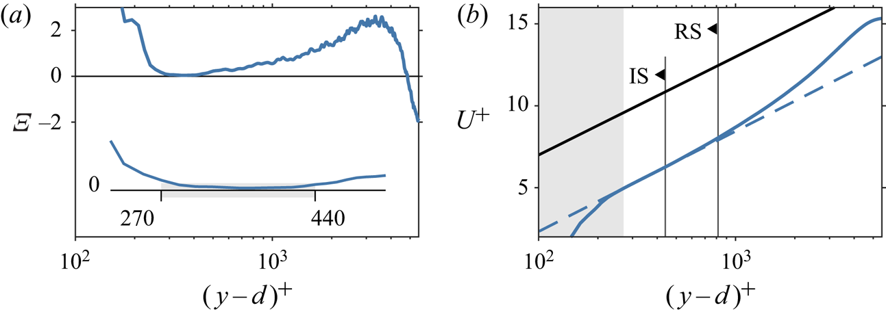
obtained by taking the partial derivative of (2.1) with respect to  $y^+$. As shown in figure 1(a), using a line search algorithm, the optimal value
 $d/h = 0.65 \pm 0.041$ (listed in table 1) was found to minimise the indicator function in the IS, defined as the region where
 $\varXi =0\pm \epsilon _{\varXi }$ with
 $\epsilon _{\varXi } = 0.02/\kappa$. This estimate is in close agreement with that obtained from surface pressure data
 $d^p = 0.619$ by Ferreira & Ganapathisubramani (Reference Ferreira and Ganapathisubramani2020b). The associated uncertainty level was estimated by conducting a linear error propagation analysis on (2.2), yielding the expression
 \begin{align} \epsilon_{d}^2 =\frac{1}{2\varDelta_{xy}^2}\left[\left(\frac{\partial U}{\partial y}\right)^{-2}\frac{U_{\tau}}{\kappa}\right]^2\epsilon_{U}^2 + \left[\left(\frac{\partial U}{\partial y}\right)^{-1}U_{\tau}\right]^2\epsilon_{\varXi}^2 + \left[ \left(\frac{\partial U}{\partial y}\right)^{-1} \frac{1}{\kappa}\right]^2\epsilon_{U_{\tau}}^2 + \varDelta_{xy}^2. \end{align}
Equation (2.3) factors the most important error contributions including uncertainties in the mean velocity data  $\epsilon _{U}$, the friction velocity
 $\epsilon _{U_{\tau }}$, the spatial resolution of the vector field
 $\varDelta _{xy}$ and the arbitrary tolerance
 $\epsilon _{\varXi }$. The wall-normal gradient of velocity was obtained via a second-order central difference scheme. An alternative, more conservative approach to this analysis is to consider
 $\epsilon _{\varXi }$ as a proxy for the uncertainty in the slope
 $\kappa$; then
 $\epsilon _{\varXi } = (1/\kappa ^2)\epsilon _{\kappa }$. Assuming
 $\epsilon _{\kappa } = 5\,\%$, the uncertainty in the zero-plane displacement becomes instead
 $0.056h$.
Estimation of the surface parameters. (a) Indicator function defined by (2.2). The inset shows a detail of the plateau corresponding to the log region where  $\varXi =0\pm \epsilon _{\varXi }$ in the range
 $(\,y-d)^+=270{-}440$. (b) Inner viscous scaling of the mean streamwise velocity profile. Dashed-blue line is the linear–log fit through the IS, with slope
 $\kappa = 0.384$, and the solid-black line is the log law for a smooth-wall boundary layer with negative zero intercept
 $A = -5$. The shaded-grey area represents the canopy region and RS the depth of the roughness sublayer.

Mean flow parameters.

Shown in figure 1(b), the IS is found within the range  $(\,y-d)^+ = 270{-}440$ and is entirely immersed within the roughness sublayer (RS), which extends up to
 $y = 1.85h$. The thickness of the RS is given here by the height above which the mean flow is horizontally homogeneous. The overlap between the two flow regions supports the hypothesis of Cheng & Castro (Reference Cheng and Castro2002) that the spatially averaged velocity profile may assume a logarithmic behaviour where turbulence is predominantly influenced by the surface geometry. Similarly, they studied the flow over cube roughness, but followed a less stringent definition to evaluate the bounds of the inertial range (based on the variation of the spatially averaged shear stress), yielding somewhat larger values than those reported here. Closer estimates would have been obtained by relaxing
 $\epsilon _{\varXi }$.
2.2. Outer-layer similarity
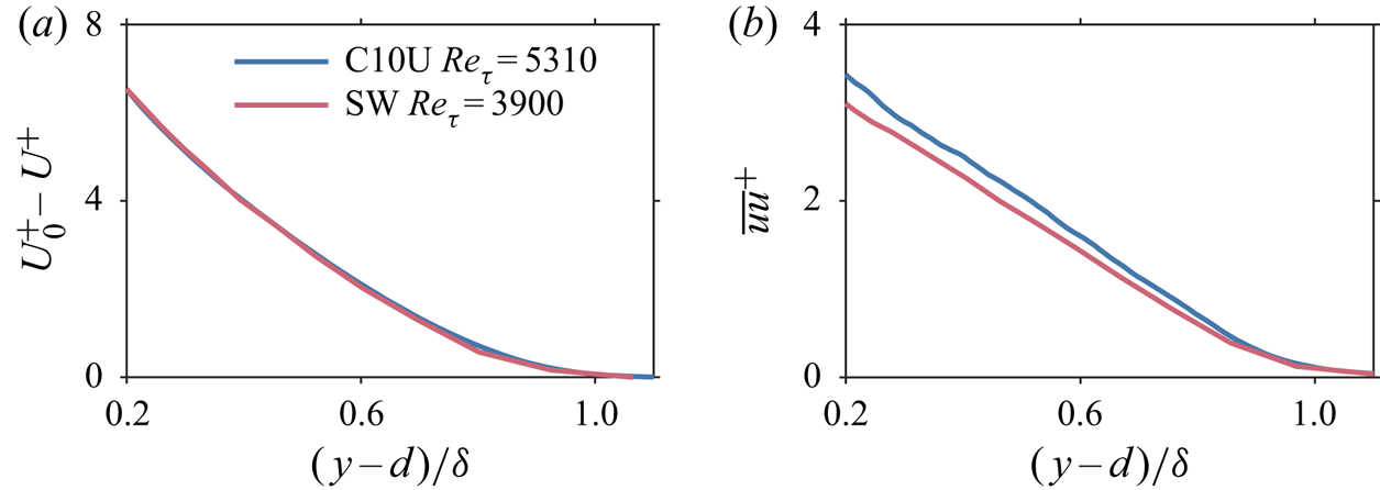
Outer similarity (Townsend Reference Townsend1976) emerges over rough walls at sufficiently high Reynolds numbers, provided the roughness length scale is a small portion of the boundary-layer thickness (Perry & Abell Reference Perry and Abell1977). Only then may the velocity profile above the canopy be expressed by a standard log-wake function that scales appropriately. As it is not yet clear what meaningful parameters better express these criteria, especially for large-cube roughness (Placidi & Ganapathisubramani Reference Placidi and Ganapathisubramani2018), the viscous-scaled velocity defect data and the streamwise turbulence stress are compared against the corresponding profiles of a smooth-wall boundary layer at a similar Reynolds number. The existence of outer similarity is evidenced in figure 2 by the remarkable collapse of the data for  $(\,y-d)/\delta >0.2$, in spite of the large relative height of the roughness obstacles (
 $\delta /h \approx 12$). Having confirmed outer-layer similarity, the roughness function could be evaluated by assuming the functional form for the viscous-scaled velocity profile of Coles (Reference Coles1953) or by means of relationship (2.1) (which implies
 ${\rm \Delta} U^+ \propto \ln y_0^+$), yielding similar results. In terms of sand-grain roughness
 $h_s^+$, both cases are well past the onset of the fully rough regime at
 $h_s^+\gtrapprox 80$ (Flack, Schultz & Connelly Reference Flack, Schultz and Connelly2007).
Outer-layer similarity. (a) Viscous scaling of the horizontal-averaged velocity deficit. (b) The viscous-scaled streamwise turbulence intensity. Hot-wire data for a smooth-wall boundary layer at  $Re_{\tau } = 3900$ were included for reference.

3. Scale decomposition
A POD-based scale decomposition of the streamwise velocity component is presented in this section. The region of interest stretches across the field of view and extends up to  $y/h=5$ (i.e.
 $0.8\delta \times 0.4\delta$). The large-scale turbulent features are characterised in terms of size and inclination angle and the effect of AM of the small scales is investigated.
3.1. POD
POD was introduced by Lumley (Reference Lumley1967) as an unbiased technique for studying coherent structures in turbulent flows. It consists in identifying a set of orthonormal functions which best correlate, in a statistical sense, with a set of observations that could either be an experimental measurement or a numerical solution of a scalar or vector field (e.g. pressure, velocity), taken at a given time. The reader is referred to Berkooz, Holmes & Lumley (Reference Berkooz, Holmes and Lumley1993) for a more rigorous explanation. Given the discrete nature of the current data set, and following the bi-orthogonal approach outlined by Aubry, Guyonnet & Lima (Reference Aubry, Guyonnet and Lima1991), each PIV snapshot of the fluctuating streamwise velocity field  $u'(\boldsymbol {x},t)$, containing
 $n_p$ point measurements, is reshaped into a row vector
 $a^{(j)} \in \mathbb {R}^{1 \times n_p}$. Here,
 $\boldsymbol {x}$ and
 $t$ are the space and time coordinates, respectively. The data set is then organised in a rectangular matrix
 $A \in \mathbb {R}^{n_t \times n_p}$, where
 $n_t$ is the total number of realisations. Since
 $n_t \ll n_p$, we consider the snapshot formulation of the discrete Fredholm equation (Sirovich Reference Sirovich1987), which is equivalent to the eigenvalue problem of the two-point, temporal correlation matrix of
 $A$, written as
 \begin{equation} AA^T\varPsi_A = \varPsi_A \varLambda, \end{equation}
with  $\varLambda =\textrm {diag}(\lambda ^{(1)},\ldots ,\lambda ^{(n_t)}) \in \mathbb {R}^{n_t \times n_t}$ containing the set of eigenvalues of
 $AA^T$ and
 $\varPsi _A = [\psi _A^{(1)},\ldots ,\psi _A^{(n_t)}] \in \mathbb {R}^{n_t \times n_t}$ the set of eigenvectors. The columns of
 $\varPsi _A$ are otherwise known as temporal modes and form the orthonormal basis for the columns of
 $A$. The spatial modes
 $\varPhi _A = [\phi _A^{(1)},\ldots ,\phi _A^{(n_t)}] \in \mathbb {R}^{n_p \times n_t}$ are then expressed as the projection of the snapshots ensemble onto the temporal modes,
 \begin{equation} \varSigma_A \varPhi_A^T = \varPsi_A^TA, \end{equation}
where  $\varSigma _A = \textrm {diag}(\sigma _A^{(1)},\ldots ,\sigma _A^{n_t}) \in \mathbb {R}^{n_t \times n_t}$ is a diagonal matrix containing the norm of each contribution and is equal to the square root of the eigenvalues
 $\varLambda$. Perret & Rivet (Reference Perret and Rivet2013) have also used POD to decompose the streamwise velocity field over a staggered-cube array. The spatial extent of their field of view is comparably smaller, but the PIV sampling frequency (5 Hz) was sufficiently high to resolve the autocorrelation function of the first temporal mode. Assuming a convection velocity, they estimated the average size of the structures associated with
 $\phi ^{(1)}$ to be approximately
 $1.2\delta$ or
 $24h$. They additionally showed that
 $\phi ^{(1)}$ contributes the most to the Reynolds shear stress in the outer region, whereas near the canopy top
 $\phi ^{(2)}$ supersedes, and found evidence of a nonlinear interaction with the high-order modes that could be AM. These results indicate that mode one bears the footprint of the low-frequency, large-scale structures. However, as recently explained by Perret & Kerhervé (Reference Perret and Kerhervé2019), it cannot alone represent their spatio-temporal dynamics for two reasons: first, because spectral aliasing is likely to occur when the flow features of interest are under-sampled; and second, because POD is unable to account for the long term coherence of the most energetic structures, which could lead to spectral mixing of different phenomena with similar energy (Towne, Schmidt & Colonius Reference Towne, Schmidt and Colonius2018). To capture the spectral content of the flow when temporal resolution is insufficient, Perret & Kerhervé (Reference Perret and Kerhervé2019) proposed a new approach based on the spectral-POD method introduced by Sieber, Paschereit & Oberleithner (Reference Sieber, Paschereit and Oberleithner2016). S-POD acts as a band-pass filter centred around a dominant frequency, determined by the characteristic time scale of the large coherent motions, thus having an anti-aliasing effect on the lower-order modes. They demonstrated that the time-signature of the first modes, which were unresolved using POD, could be improved, and were shown to be associated with LSMs.
In contrast to Perret & Kerhervé (Reference Perret and Kerhervé2019), the current data set is statistically uncorrelated, so it does not contain any useful time information. The present scale decomposition is then subject to the above-mentioned limitations that could be detrimental to an accurate characterisation and quantification of the flow processes. Nevertheless, as shown in the following section, a POD-based approach appears to perform adequately in capturing the large-scale structure and inter-scale dynamics.
3.2. Large-scale coherent structures
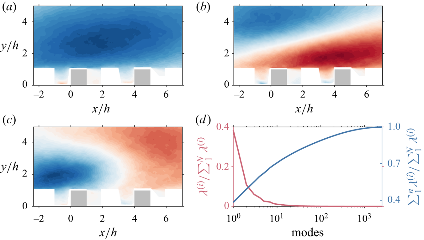
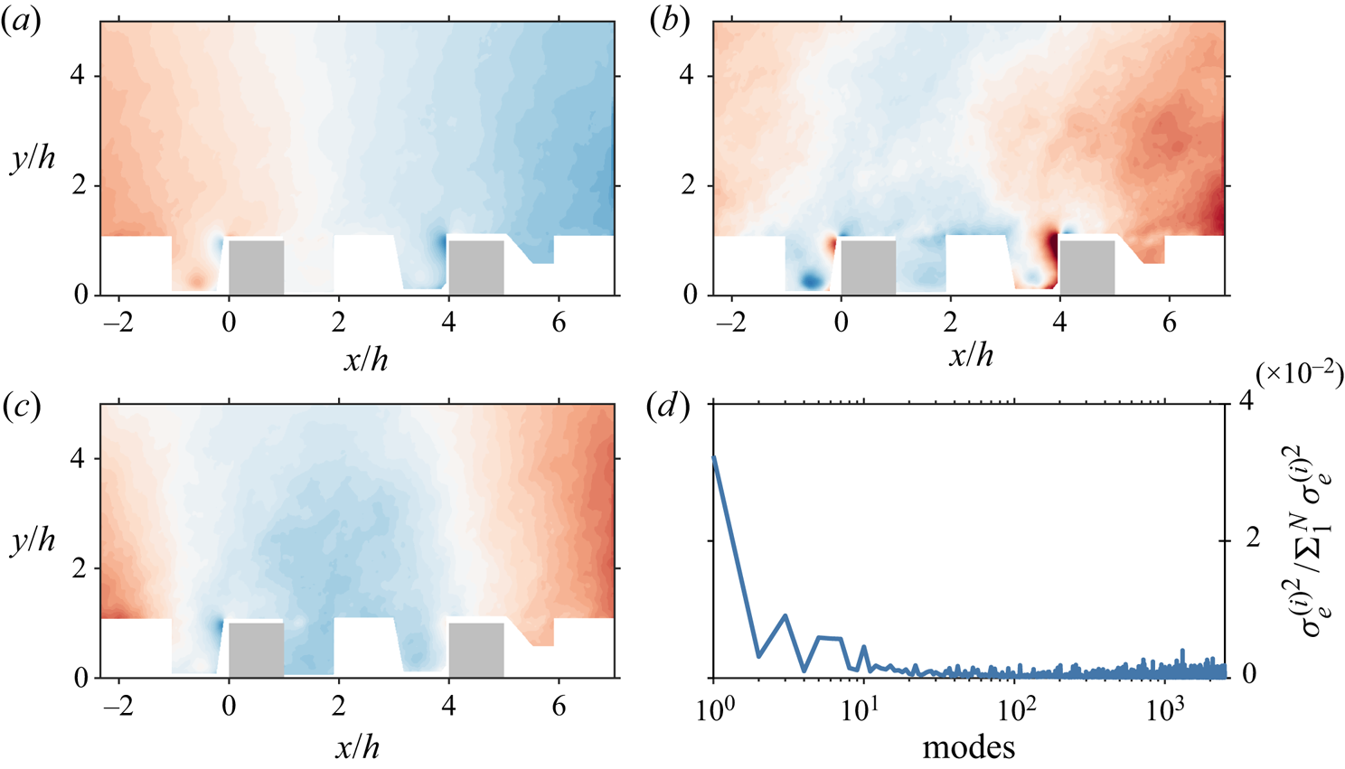
Represented in figure 3(a), the first POD mode shape reveals a streamwise-elongated, forward-leaning feature spanning across the measurement domain, presumably associated with LSMs of high and low momentum. The second and third mode shapes correspond to events of smaller wavelength, but may still be important to correctly capture the dynamics of the largest structures. The energy convergence of the POD modes is shown in figure 3(d). Remarkably, the first contains nearly  $40\,\%$ of the overall streamwise turbulent kinetic energy, far more than any other, and the contribution of the first ten modes (out of
 $2500$) exceeds
 $70\,\%$.
POD of the flow field. First three spatial POD modes,  $\phi _A^{1}$ (a),
 $\phi _A^{2}$ (b) and
 $\phi _A^{3}$ (c). Red- and blue-shaded regions correspond to positive and negative streamwise velocity fluctuations, respectively. Obstacles in the measurement plane are highlighted grey. (d) The cumulative energy contribution of the flow field modes (on the right-vertical axis).

The integral length scale  $L_x$ is estimated by fitting an exponential decaying function of the form
 $k\exp ({-{\rm \Delta} x/L_x})$ to the spatial velocity correlation (e.g. Reynolds & Castro Reference Reynolds and Castro2008), defined by
 \begin{equation} R_{uu}(\boldsymbol{x})= \frac{\langle u(\boldsymbol{x},t)u(\boldsymbol{x}+{\rm \Delta}\boldsymbol{x},t) \rangle}{\sigma_{u}(\boldsymbol{x}) \sigma_{u}(\boldsymbol{x}+{\rm \Delta}\boldsymbol{x})}, \end{equation}
where  $\langle \cdot \rangle$ is the ensemble average operator,
 $\Delta \boldsymbol {x}$ is the separation between ‘probes’ and
 $\sigma _u(\boldsymbol {x})$ is the standard deviation of the velocity field. The streamwise distribution of
 $R_{uu}$ at a fixed reference height
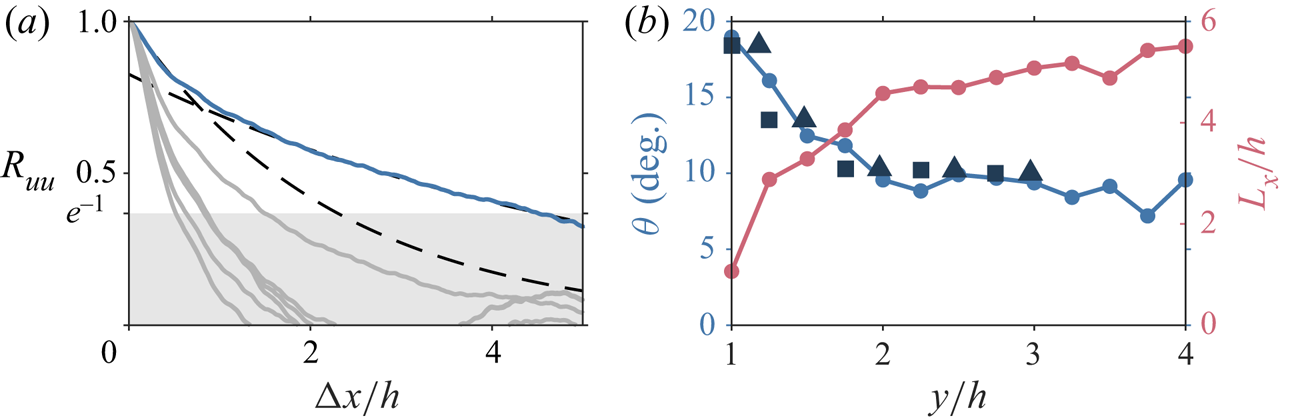
 $y/h=2$ is given in figure 4(a), evidencing the two-scale behaviour reported by Castro, Cheng & Reynolds (Reference Castro, Cheng and Reynolds2006). The correlation function can be fitted by two exponentials with decay constants differing by a factor of two:
 $L_x/h = 2.3$ for
 ${{\rm \Delta} x/h<1}$ and
 $L_x/h = 5.6$ for larger horizontal probe separations. At greater heights, however, the effect of the shear layers on the turbulence dynamics fades away and the flow exhibits instead one dominant scale. The correlation function is then adequately fit by a single exponential (not shown here). Additional curves were obtained for the same location by gradually removing the most energetic POD modes from the reconstruction of the velocity fields. The results emphasise the link between the first mode and the large-scale events, as
 $L_x$ (given by the larger dominant scale) drops from about
 $5.6h$ to less than
 $2h$ if only higher-order modes corresponding to events of smaller wavelength are retained.
Morphometrics of the coherent structures. (a) Two-point streamwise velocity correlation  $R_{uu}$ for a fixed reference height
 $y/h = 2$ within the RS (solid-blue line). The black dash-dotted lines are exponential curves of the form
 $k\exp ({-{\rm \Delta} x/L_x})$ with
 $L_x/h = 2.3$ for
 ${\rm \Delta} x/h<1$ and
 $L_x/h = 5.6$ for
 ${\rm \Delta} x/h>1$. Solid-grey lines are correlations obtained for the same reference location by gradually removing the most energetic POD modes from the reconstruction of the velocity fields. (b) The angle of inclination
 $\theta$ of the structures (on the left-vertical axis) and the integral-length scale
 $L_x$ (on the right-vertical axis) against the wall-normal location of the reference probe. Measurements of
 $\theta$ from Castro et al. (Reference Castro, Cheng and Reynolds2006) (squares) and Reynolds & Castro (Reference Reynolds and Castro2008) (triangles) were included for reference.

The size  $L_x$ and typical inclination angle of the structures
 $\theta$ are plotted against the vertical coordinate in figure 4(b), with
 $\theta$ expressed as the rotation angle of the principal axes of the contour level
 $R_{uu} = \textrm {e}^{-1}$ relative to the wall. The integral length scale increases from
 $1.1h$ at the canopy top to
 $5.5h$ at
 $y/h = 4$. This is consistent with results from Castro et al. (Reference Castro, Cheng and Reynolds2006), Coceal et al. (Reference Coceal, Dobre, Thomas and Belcher2007) and Reynolds & Castro (Reference Reynolds and Castro2008) under similar flow conditions, in the sense that, immediately above the canopy, scales are expected to be of the order of the cube height, but are instead associated with the depth of the boundary layer away from the wall. Specifically,
 $L_x/\delta = 0.40{-}0.45$ in the outer region (
 $y/h>2.5$), which closely matches the values reported by Ganapathisubramani et al. (Reference Ganapathisubramani, Hutchins, Hambleton, Longmire and Marusic2005), for the smooth-wall case (
 $0.42$ at
 $y/\delta = 0.5$), and Reynolds & Castro (Reference Reynolds and Castro2008) for cube roughness (
 $0.44$). The angle of inclination sharply decreases from
 $19^{\circ }$ at
 $y/h = 1$ to
 $10^{\circ }$ at
 $y/h = 2$, thereafter decreasing marginally to approximately
 $8^{\circ }$. This behaviour is opposite to the smooth-wall counterpart, where the LSMs are inclined at a shallow angle near the wall and lift away with increasing height (e.g. Marusic Reference Marusic2001; Ganapathisubramani et al. Reference Ganapathisubramani, Hutchins, Hambleton, Longmire and Marusic2005). Krogstad & Antonia (Reference Krogstad and Antonia1994) had previously reported this behavioural change, owing to the large wall-normal velocity fluctuations over the surface. A more elaborate explanation was proposed by Coceal et al. (Reference Coceal, Dobre, Thomas and Belcher2007), in terms of the basic structural elements of the hairpin-packet model of Adrian, Meinhart & Tomkins (Reference Adrian, Meinhart and Tomkins2000), of which they found evidence on instantaneous snapshots of the filtered data and by conditionally averaging the flow field. They suggest that the larger distance between hairpin vortices and their symmetric part (i.e. the image vortex) causes the self-induction upwards by the legs of the vortex to become stronger relative to the mean shear effect (that contributes to align and stretch vorticity in the streamwise direction). The decreasing trend in
 $\theta$ is thus associated with a more rapid decrease of the self-induction as compared to the decrease of the mean shear.
3.3. Scale interactions
To assess the existence of AM, we consider the expansion of the streamwise velocity skewness  $S_u = \langle {u'}^3\rangle /(\langle {u'}^2\rangle ^{3/2})$ using the scale decomposed velocity signal
 $u' = u'_L + u'_S$, where
 $u'_L$ and
 $u'_S$ are the large and the small-scale components of
 $u'$, respectively. The third-order moment of the streamwise velocity then reads
 \begin{equation} \langle {u'}^3 \rangle = \langle {u'_L}^3 \rangle + 3\langle {u'_L}^2u'_S \rangle + 3\langle {u'_S}^2u'_L \rangle + \langle {u'_S}^3 \rangle \end{equation}
with
 \begin{equation} u'_L = \sum_{i=1}^{n}\psi_A^{(i)} \sigma_A^{(i)} {\phi_A^{(i)}}^\textrm{T}, \end{equation}
where  $n$ is the number of POD modes retained in the reconstruction of the velocity signal
 $u'_L \in \mathbb {R}^{n_t \times n_p}$, which contains the large-scale fluctuation at each measurement point and temporal realisation, organised similarly to
 $u'(\boldsymbol {x},t)$ in
 $A$. There is substantial evidence to suggest that the scale-decomposed skewness factor is closely related with AM effects (Sreenivasan, Dhruva & Gil Reference Sreenivasan, Dhruva and Gil1999; Schlatter & Örlü Reference Schlatter and Örlü2010; Mathis et al. Reference Mathis, Marusic, Hutchins and Sreenivasan2011b). Specifically, Mathis et al. (Reference Mathis, Marusic, Hutchins and Sreenivasan2011b) showed that the cross-term
 $\langle {u'_S}^2u'_L \rangle$ can be used as an alternative diagnostic tool to a more complex procedure, based on the correlation between the filtered envelope of the small-scale fluctuations and the large-scale signal (Mathis, Hutchins & Marusic Reference Mathis, Hutchins and Marusic2011a). This approach is especially useful when time-resolved velocity measurements are unavailable and, despite its intrinsic limitations, it has been shown to provide a good qualitative measure of the degree of AM (e.g. Perret & Savory Reference Perret and Savory2013; Perret & Rivet Reference Perret and Rivet2013; Blackman & Perret Reference Blackman and Perret2016).
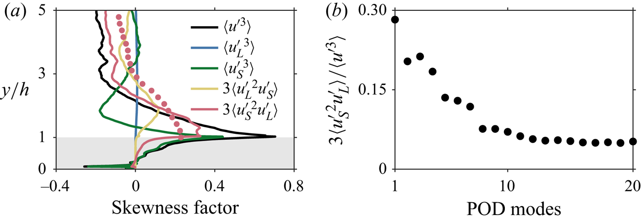
The wall-normal evolution of the terms on the right-hand side of (3.4) for  $n=1$ are shown in figure 5(a). Profiles were streamwise averaged over a repeating unit, at the centre plane of the cubes. Apart from
 $\langle {u'_L}^3 \rangle$ which is nominally zero throughout the inner region of the boundary layer, all remaining terms have a non-negligible contribution. The small-scale term
 $\langle {u'_S}^3 \rangle$ accounts for the majority of the skewness factor below the edge of the canopy, since the shear-layer interface provides a high degree of sheltering of the flow within from that above (refer to figure 3a). It then decreases with height in the RS, becoming negative at around the mid-point of the logarithmic region. The cross-term
 $\langle {u'_S}^2u'_L \rangle$ is most significant above the canopy, within the roughness-affected layer, indicating the existence of a nonlinear interaction mechanism that could be AM of the small scales under the influence of large structures. In a similar manner, the fact that
 $\langle {u'_L}^2u'_S \rangle$ is non-negligible could suggest an equivalent feedback mechanism through which the large scales are modified (Perret & Rivet Reference Perret and Rivet2013). Blackman & Perret (Reference Blackman and Perret2016) have shown, however, that this is likely an artefact of the POD scale decomposition, which is energy driven as opposed to time or spectral-based filters. Consequently, lower-order modes, typically associated with large-scale structures, encompass part of the small-scale energy as well. Figure 5(a) also includes the component of the skewness
 $\langle {u'_S}^2u'_L \rangle$ estimated by Perret & Kerhervé (Reference Perret and Kerhervé2019) using S-POD. The data exhibit a similar trend, but the cross-over point is farther away from the wall and the magnitude is comparably smaller, owing to a different scale separation and energy distribution across the modes.
Scale interaction. (a) Components of the scale-decomposed skewness factor  $S_u$ for
 $n=1$ (3.4). The estimate of
 $3\langle {u'_S}^2u'_L \rangle$ by Perret & Kerhervé (Reference Perret and Kerhervé2019) is indicated by the red symbols. All terms are normalised by
 $\sigma _u^{3/2}$. (b) Cross-term
 $3\langle {u'_S}^2u'_L \rangle$ at
 $y/h = 1.5$ as a function of the number of POD modes retained in the reconstruction of the large-scale velocity signal.

To further elucidate the scale characteristics of the POD modes, the cross-term  $\langle {u'_S}^2u'_L \rangle$ of the scale-decomposed skewness factor, at
 $y/h = 1.5$, is plotted in figure 5(b) against the number of POD modes retained in the reconstruction of the large-scale velocity signal. The results show a decreasing trend in the correlation level as
 $u'_L$ gradually combines higher-order modes, varying marginally for
 $n>10$. This would be expected given that
 $\langle {u'_S}^2u'_L \rangle$ accounts not only for the modulation effect but also for the small-scale variance, which becomes gradually smaller with
 $n$. The impact on AM only becomes apparent because the evolution is not monotonic, suggesting that the most energetic modes (at least up to
 $n=3$) have a non-negligible contribution. A more rigorous analysis is provided by Perret & Kerhervé (Reference Perret and Kerhervé2019), who demonstrated that multiple lower-order modes are required to fully capture the spectral content of the large structures and the inter-scale dynamics (§ 3.1). Still, using mode one alone to model the large-scale signal appears to provide already a good qualitative agreement with published data.
4. Surface drag characteristics
The force experienced by a target roughness element located at  $x/h=0$ is used here as a proxy for the local wall shear stress. Instantaneous maps of the pressure field obtained from snapshot PIV were used to estimate the axial load
 $F = F_{w}-F_{l}$, where the subscript identifies the windward (
 $F_{w}$) and leeward (
 $F_{l}$) sides of the cube. The height of the centre of pressure
 $y_{cp}$ could also be determined, whose mean value, according to Jackson (Reference Jackson1981), would correspond to the zero-plane displacement
 $d^{p}$. Note that the uncertainty associated with
 $y_{cp}$ is inversely related to
 $F$ (refer to (2.3)), causing estimates of
 $y_{cp}$ to exceed
 $h$ in a few instances that were omitted from the following analysis. Force statistics and conditional averages of the flow field are presented in this section to provide some insight into the canopy-drag behaviour and the relevant flow phenomena.
4.1. Force statistics
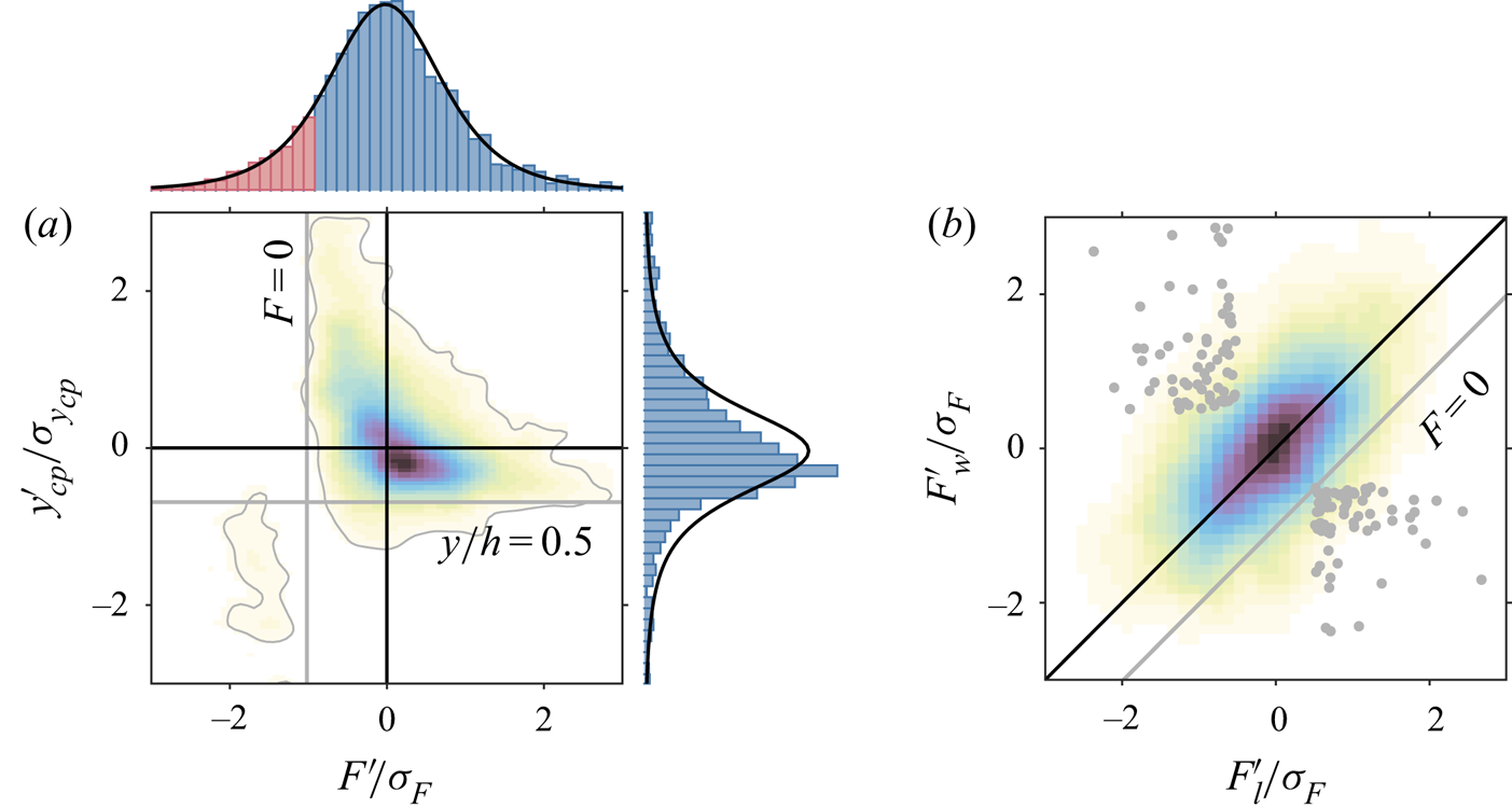
The joint-probability density function (JPDF) of the fluctuating force and height of the centre of pressure, normalised by the corresponding standard deviations,  $\sigma _{F}$ and
 $\sigma _{y_{cp}}$, is shown in figure 6(a) alongside each individual probability density function (PDF). Notably, the force exhibits a Gaussian distribution, with frequent negative-drag or thrust-producing events that amount to nearly
 $13\,\%$. This value is greater than
 $0.1\,\%$ reported for smooth walls (Alfredsson et al. Reference Alfredsson, Johansson, Haritonidis and Eckelmann1988; Örlü & Schlatter Reference Örlü and Schlatter2011) and stems from the different nature of the canopy drag that is predominantly pressure based. Although negative-drag events would be expected, they have mostly been observed on particle-bed studies (e.g. Cameron, Nikora & Marusic Reference Cameron, Nikora and Marusic2019), wherein the force is traditionally measured via direct methods. It is also evident that the roughness obstacles experience extreme excursions of the force, with a r.m.s. level of approximately
 $140\,\%$ of the mean value, against
 $40\,\%$ over smooth walls (Alfredsson et al. Reference Alfredsson, Johansson, Haritonidis and Eckelmann1988).
Drag force statistics. (a) Two-dimensional JPDF of the fluctuating force  $F'$ and the height of the centre of pressure
 $y'_{cp}$, normalised by the standard deviations
 $\sigma _{F}$ and
 $\sigma _{y_{cp}}$, respectively. The solid-grey lines indicate the cube half height (horizontal) and the zero crossing of the force (vertical). PDF of
 $F'$ (on top) and
 $y'_{cp}$ (on the right) overlaid with the corresponding Gaussian distributions (solid-black lines). (b) Two-dimensional JPDF of the fluctuating force on the windward
 $F'_w$ and leeward
 $F'_l$ sides of the cube. Along the solid-black line, the total force remains unchanged and equal to the mean value. Thrust-producing events lie below the solid-grey line. Grey markers represent the
 $F'$ pairs associated with (4.1).

The height of the centre of pressure shows a skewed distribution towards the edge of the cube with a standard deviation  $\sigma _{y_{cp}}/h = 0.14$. The force tends to act for the most part below the zero-plane displacement height (
 $55\,\%$), albeit occasionally on the lower half of the cube for thrust-producing events. Positive deviations of
 $y_{cp}$ exhibit a broader distribution, in some cases approaching the top of the cube, but are generally associated with the least intense force fluctuations. This could be explained by the passage of small-scale turbulent pressure fluctuations associated with the shear layer, which leave an imprint on the upper half of the cube. Large-scale events, on the other hand, are more likely to affect uniformly the pressure field within the canopy layer, causing the centre of pressure to lie at approximately half-height.
The JPDF of the forces acting on the windward and leeward sides of the target roughness obstacle is given in figure 6(b), normalised by the standard deviation of the total force  $\sigma _F$. These quantities reveal a strong positive correlation
 $R_{F_{w}F_{l}} = 0.59$ and similar amplitudes, suggesting the existence of an underlying, advecting pressure wave that evenly affects the flow field over a wide region. The most extreme excursions of the force on either side of the cube partially or entirely cancel each other out, so the less intense, anti-signed events corresponding to the second and fourth quadrants of the plane (
 $F'_{w}$,
 $F'_{l}$) are the most important to the surface drag fluctuations.
4.2. Conditional averages
In view of the above results, we examine the conditional averages of the fluctuating velocity field  $\boldsymbol {u'(x)}$ based on the loading combination upstream and downstream of the target element located at
 $x/h= 0$, defined as
 \begin{equation} \left.\begin{gathered} \widetilde{\boldsymbol{u'}}\mid_{h} (\boldsymbol{x}) = \langle \boldsymbol{u'} \mid F'_w/\sigma_F>0.5 \cap F'_l/\sigma_F<-0.5\rangle \\ \text{and} \\ \widetilde{\boldsymbol{u'}}\mid_{l} (\boldsymbol{x})= \langle \boldsymbol{u'} \mid F'_w/\sigma_F<-0.5 \cap F'_l/\sigma_F>0.5\rangle, \end{gathered}\right\} \end{equation}
as well as of the pressure coefficient  $\tilde {C}_{p'}\boldsymbol {(x)}$. The
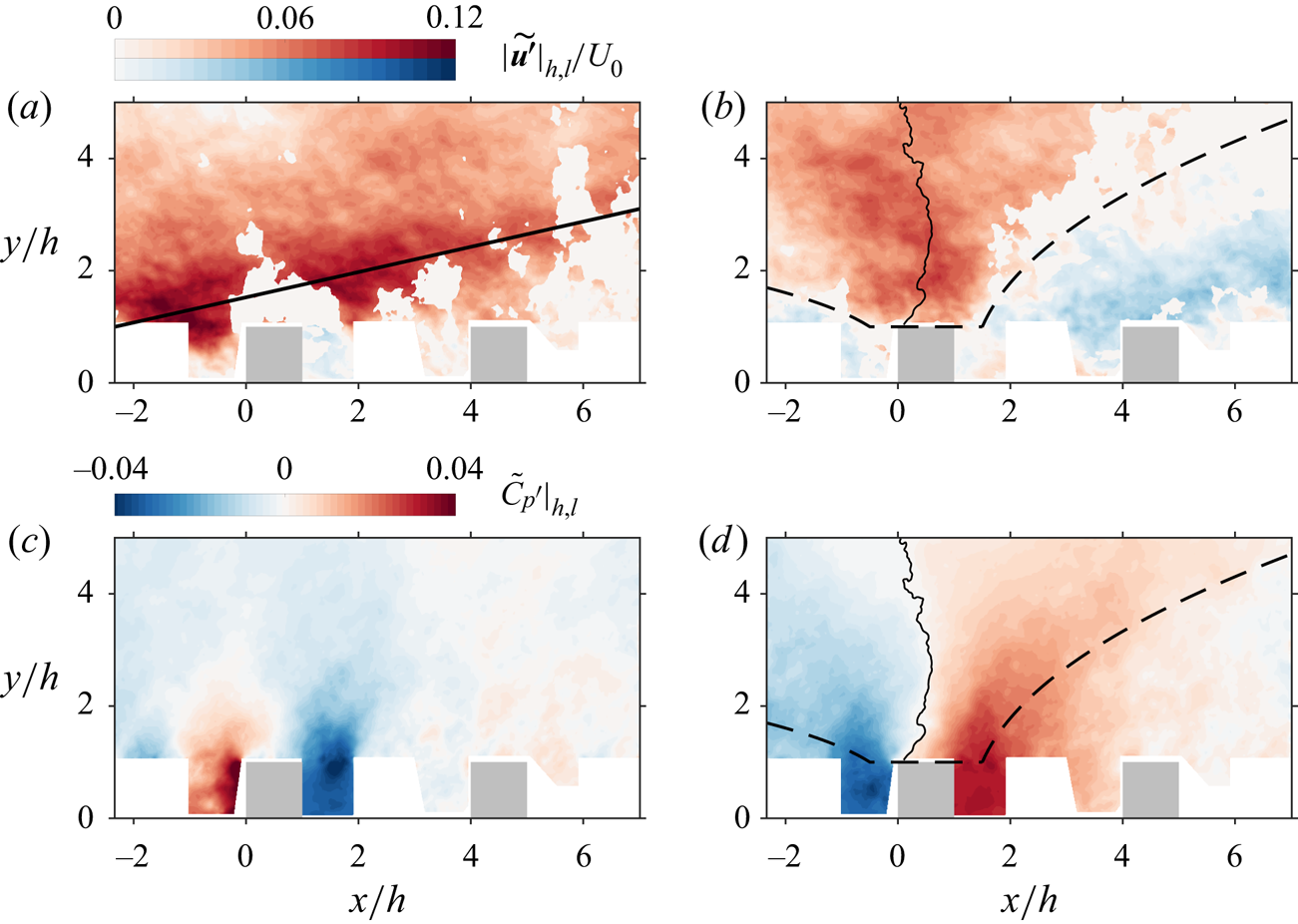
 $F'$ pairs corresponding to the conditions above are highlighted grey in figure 6(b). The magnitude of the conditional-averaged velocity fluctuations
 $|\widetilde {\boldsymbol {u'}}|$ is shown in figure 7(a,b) for positive and negative excursions of the force, respectively. Shades of blue indicate low-velocity outward motions, ejections or
 $Q2$ events, and shades of red indicate high-velocity inward motions, sweeps or
 $Q4$ events, that contribute the most to the wall-normal exchange of momentum between the canopy and the flow aloft. At the bottom, figure 7(c,d) are the corresponding conditional averages of the pressure coefficient.
Conditional structure of the boundary layer on high- and low-drag events. Maps of the fluctuating velocity magnitude  $|\widetilde {\boldsymbol {u'}}|$ (on top) and the pressure coefficient
 $\tilde {C}_{p'}$ (at the bottom). (a,c) Are conditionally averaged on a high (
 $h$) drag event and (b,d) on a low (
 $l$) drag event. Different colour maps of velocity are for sweeps (shades of red) and ejections (shades of blue). Regions of
 $Q1$ and
 $Q3$ events are plotted in white. The solid-black line in (a) represents the average inclination angle of the structure at
 $13^{\circ }$. Dashed and solid-back lines in (b) and (d) indicate, respectively, the shear-layer interface between the sweeping motion and ejections, and the local minima of the conditioned pressure fluctuations.

For positive-drag fluctuations, a high-momentum LSM is clearly visible, similar in shape to the first POD mode. It lies at an average inclination angle of approximately  $13^{\circ }$, in agreement with values estimated from two-point spatial correlations (refer to figure 4b). The large pressure difference appears to arise mostly from the sweeping motion impinging on the surface roughness, as the fluid is pushed against the windward side of the cube, creating a highly turbulent region just below the canopy top. It is then deflected upwards and over, giving rise to a
 $Q1$ event (
 $u'>0, v'>0$) immediately above, which in turn contributes to reduce the static pressure in the wake.
A careful examination of figures 7(b)–7(d) reveals that the mechanism responsible for negative-drag fluctuations is markedly different. High and low-pressure regions are noticeably broader, and appear to be associated with the large-scale outward and inward interactions. More precisely, the conditional flow structure is characterised by a large shear layer that extends across the entire field of view, indicated by the dashed-black line. Downstream of the roughness obstacle, this interface is positively inclined and there is a local increase of the static pressure as the flow is squeezed between the sweep and ejection regions. Within the canopy, the upward flow expands and the turbulent shear layer occupies a wider region, shedding small-scale structures into the RS and thereby losing significance. In contrast, the interface is negatively inclined upstream of the cube,  $x/h<0$, and pressure is locally reduced. The relative inclination angle is important as it determines the nature of the interaction, which is one of pure shear and relatively less energetic.
Although we conditionally averaged the flow field based on the force signal to identify relevant flow phenomena, similar patterns have been observed for different rough-wall boundary layers using distinct approaches, substantiating the present analysis. For example, Zhu, van Hout & Katz (Reference Zhu, van Hout and Katz2007) found that during sweep motions the turbulent kinetic energy, Reynolds stresses and production/dissipation rates, have clear narrow peaks just below the canopy height. This scenario would presumably be equivalent to that conditioned to a positive force fluctuation. In turn, during ejections, these variables exhibit a broad maxima above the canopy, contributing to reduce the energy content within. This would then explain the lower pressure value on the windward face of the cube for a condition of low drag. There is also a significant resemblance between the conditional flow structure in figure 7(b) and a bursting event that is a prime contributor to turbulence production (e.g. Runstadler, Kline & Reynolds Reference Runstadler, Kline and Reynolds1963; Kline et al. Reference Kline, Reynolds, Schraub and Runstadler1967). Several definitions have been proposed, most of which were comprehensively reviewed by Robinson (Reference Robinson1991). The phenomenon is typically characterised by violent outward eruptions of near-wall fluid and features a shear-layer interface that develops in-between an upstream, high-speed sweep and a downstream, low-speed ejection. Thomas & Bull (Reference Thomas and Bull1983) studied the interrelation between wall pressure fluctuations and the burst–sweep cycle in the buffer region of a smooth-wall boundary layer. They showed that an increase in pressure is generally associated with the passage of inclined shear layers that occur on the upstream side of the bursting process, and that it may traverse most of the boundary-layer thickness. This effect is visible too in figure 7(d).
Of particular interest are the minima of the magnitude of the conditional-averaged pressure fluctuations, represented by the solid-black line in figures 7(b)–7(d). On closer inspection, it becomes evident that it lies in a sweeping region where the velocity fluctuations are most intense. This implies that, upstream of the contour line, where pressure is low, the flow is predominantly accelerated ( $\partial \boldsymbol {u'}/\partial \boldsymbol {x}>0$), whereas, in the region downstream, an increase in pressure is accompanied by a local deceleration (
 $\partial \boldsymbol {u'}/\partial \boldsymbol {x}<0$). A similar analysis was carried out by Hutchins et al. (Reference Hutchins, Monty, Ganapathisubramani, Ng and Marusic2011) for a smooth-wall boundary layer. Tracing the separation between increased and reduced small-scale activity, they found that the small-scale energy attenuation or amplification is generally aligned with LSMs exhibiting local positive or negative accelerations, respectively.
5. Velocity–pressure interrelations
The influence of the large scales populating the RS is widespread. In addition to leaving a footprint onto the near-wall turbulence, via superposition of energy and AM of the small-scale dynamics, the conditional analysis shows evidence that pressure may be equally affected. It is then reasonable to assume they have direct implications on the surface drag characteristics of rough-wall boundary layers, as they do over smooth walls. Following the scale decomposition of the streamwise velocity field presented in § 3, we examine here this potential link, as well as the role of AM on drag production.
5.1. Pressure signature of the large scales
The linear relationship between the pressure field  $p$ and the large-scale, streamwise velocity fluctuations
 $u'_L = \psi ^{(1)}\sigma ^{(1)}{\phi ^{(1)}}^\textrm {T}$ is expressed by the correlation function
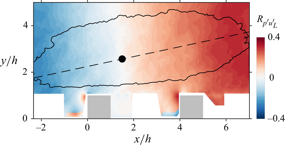
 \begin{equation} R_{p'u'_L}(\boldsymbol{x})= \langle {u'}_L(\boldsymbol{x},t){p'}(\boldsymbol{x},t) \rangle/(\sigma_{u'_L}(\boldsymbol{x})\sigma_{p'}(\boldsymbol{x})), \end{equation}
where  $\sigma _{u_L}$ and
 $\sigma _{p}$ are the corresponding standard deviations. It is represented in figure 8, overlaid with an arbitrary contour line and the locus of the first POD mode shape (given in figure 3(a) to illustrate the phase relationship between a large scale event and pressure. The correlation function is fairly uniform along the vertical direction, but monotonically increases with downstream distance, suggesting that high-momentum regions typically experience an adverse pressure gradient (
 $\partial p/\partial x>0$), while low-momentum regions are instead subject to favourable pressure gradients (
 $\partial p/\partial x<0$). The correlation value is predominantly negative in the upstream region, becoming positive farther downstream. The zero crossing is incidentally aligned with the locus of the coherent motion, where the local extrema of the velocity fluctuations lie (i.e. minima or maxima), demarcating a region of acceleration (
 $\partial \boldsymbol {u'}/\partial \boldsymbol {x}>0$) from one of deceleration (
 $\partial \boldsymbol {u'}/\partial \boldsymbol {x}<0$). For example, in the advent of a high-momentum LSM, the flow experiences a local acceleration upstream from the reference point and a deceleration downstream. Figure 8 thus seems to indicate that an increase in local static pressure is associated with flow regions that exhibit a local deceleration and, conversely, a decrease in pressure is associated with regions exhibiting a local acceleration.
Pressure signature of large coherent structures. Correlation function between the coefficients of the first POD mode, corresponding to the large-scale streamwise velocity fluctuations, and the pressure field  $R_{p'u'_L}$. An arbitrary contour line and locus of the first POD mode shape are indicated by the solid-black line and by the filled-black circle, respectively. The average inclination of the structure at
 $13^{\circ }$ is given by the dashed-black line.

It is also evident that pressure fluctuations are greatest around the extremities of the structure, at the interface between high- and low-momentum regions, where accelerations (in absolute terms) are statistically most intense. This is in agreement with figures 7(b)–7(d), as well as with results by Thomas & Bull (Reference Thomas and Bull1983), who analysed the phase relationship between the velocity and surface pressure variations within a smooth-wall boundary layer. They noticed that the amplitude of the pressure fluctuations would vary with the velocity gradient across the shear layer upstream of a bursting event if the time lag arising from its inclination angle was taken into account. Further analyses carried out by Johansson et al. (Reference Johansson, Her and Haritonidis1987), Naguib, Wark & Juckenhöfel (Reference Naguib, Wark and Juckenhöfel2001) and Naka et al. (Reference Naka, Stanislas, Foucaut, Coudert, Laval and Obi2015) show consistent results, with the wall pressure peak aligned with the centre of the shear layer. Note that although we here focus on the first POD mode alone, the same trends were observed for smaller turbulent features.
The pressure signature of the large scales additionally offers a sensible explanation for the JPDF of the fluctuating force acting on opposite sides of a cube, shown in figure 6(b). The correlation map resembles a pressure wave whose length is several times larger than  $h$. As it advects downstream, the forces on the windward and leeward sides fluctuate accordingly. However, since the wavelength is considerably larger than the width of a cube, the total force
 $F$ varies only slightly in response to changes in background pressure from the passage of coherent structures – along the diagonal line featured in figure 6(b)
 $F$ remains unchanged. This is reflected on the correlation coefficient between
 $u'_L$ and
 $F'$ that is only
 $R_{F'u'_L}=0.064$. To confirm this observation, there remains to determine if the most extreme excursions of the force on either side of the roughness obstacle are in fact associated with this pressure mode. The force signals
 $F'_w$ and
 $F'_l$ are expected to be out-of-phase by
 ${\rm \pi} /2$ with respect to
 $u'_L$, as pressure fluctuations are larger at the interface between low- and high-momentum regions. Consequently, the correlation coefficients at zero lag are relatively small (
 $R_{F'_wu'_L}=0.063$ and
 $R_{F'_lu'_L}=0.01$). A different approach must then be considered, which allows to circumvent the lack of phase information. This is achieved in the following section using extended proper orthogonal decomposition (EPOD) to extract the part of the pressure field correlated with each turbulent flow feature (i.e. POD mode of the velocity data set).
5.2. Extended POD analysis
EPOD was formally introduced by Borée (Reference Borée2003) as a statistical tool to analyse correlated events in turbulent flows which may or may not be of the same nature. Maurel, Borée & Lumley (Reference Maurel, Borée and Lumley2001), for example, investigated the jet–vortex interaction in a model engine cylinder using EPOD to identify the relevant flow phenomena driving the vortex formation. These only marginally contribute to the total kinetic energy in the flow, so POD performed over the entire domain would have not yielded useful results. In a different manner, Antoranz et al. (Reference Antoranz, Ianiro, Flores and García-Villalba2018) recently used EPOD to study and quantify the contribution of velocity modes to the turbulent heat transport in a pipe flow. Their analysis is based on velocity and temperature data from a direct numerical simulation. Specifically, in this context, we analyse the correlation of the fluctuating pressure field with the projection of the velocity field on the POD modes presented in § 3. This is possible because the pressure signal  $B \in \mathbb {R}^{n_t \times n_p}$ was inferred from instantaneous snapshots of velocity data
 $A \in \mathbb {R}^{n_t \times n_p}$ and thus have the same time evolution. The extended pressure modes are obtained by projecting
 $B$ onto the temporal basis
 $\varPsi _A$, as in Borée (Reference Borée2003). It follows that
 \begin{equation} \varSigma_e \varPhi_e^T = \varPsi_A^TB, \end{equation}
where  $\varSigma _e = \textrm {diag}(\sigma _e^{(1)},\ldots ,\sigma _e^{r}) \in \mathbb {R}^{r \times r}$ is a diagonal matrix containing the norm of the projection of
 $B$ on each temporal mode of
 $A$, and
 $\varPhi _e = [\phi _e^{(1)},\ldots ,\phi _e{(r)}] \in \mathbb {R}^{n_p \times r}$ are the EPOD modes of pressure. The square of
 $\sigma _e^{(i)}$ accounts only for the part of the pressure variance correlated with the temporal mode
 $(i)$ of the velocity signal, providing a measure of the magnitude of the pressure fluctuations associated with each turbulent scale. The EPOD modes are ordered after the POD velocity modes and not by descending energy content.
Figures 9(a)–9(c) show the first three EPOD mode shapes, which represent the part of the pressure signal that is directly correlated with the corresponding POD modes of velocity. Since the large-scale velocity signal is expressed by  $u'_L = \psi ^{(1)}\sigma ^{(1)}{\phi ^{(1)}}^\textrm {T}$, it is unsurprising that
 $\phi _e^{(1)}$ (figure 9a) closely resembles the correlation function
 $R_{p'u'_L}$. If the first POD mode of velocity
 $\phi ^{(1)}$ (figure 3a) is overlaid on
 $\phi _e^{(1)}$, it becomes apparent that the pressure field is positively correlated with the streamwise component of the velocity fluctuations downstream of the coherent structure, but instead exhibits an anti-signed behaviour upstream. This relationship is noticeable too for higher-order modes, albeit to a lesser extent. More importantly, the magnitude of the eigenvalues of the EPOD modes provides a measure of their relative importance to the fluctuating pressure field. Shown in figure 9(d), the relative contribution of
 $\phi _e^{(1)}$ to the total pressure variance is by far the largest, although it only amounts to a small fraction (approximately
 $3\,\%$). The bulk part appears to be distributed over higher-order modes, which show a small but non-negligible contribution.
EPOD modes of pressure. First three extended pressure modes on the velocity basis,  $\phi _e^{(1)}$ (a),
 $\phi _e^{(2)}$ (b) and
 $\phi _e^{(3)}$ (c). The red and blue-shaded regions correspond to positive and negative pressure fluctuations, respectively. (d) The relative contribution of the EPOD modes to the overall pressure fluctuations.

The present results establish a link between  $\phi ^{(1)}$, associated with the large coherent structures, and
 $\phi _e^{(1)}$, which is the single greatest contributor to the fluctuating pressure field. Considering the strong coupling between the forces acting on the windward and leeward sides of a cube (
 $R_{F'_{w}F'_{l}} = 0.59$), it is then reasonable to conclude that the most extreme excursions of these forces are the imprint of a broad advecting pressure wave associated with the passage of alternating high- and low-momentum regions. As a first-order approximation
 $R_{F'_{w}F'_{l}} \propto L_x/h$, suggesting that the significance of the large coherent structures to surface drag is mitigated by the relatively small size of the obstacles compared to the integral length scale. In a different context, Cameron et al. (Reference Cameron, Nikora and Marusic2019) have recently reported a possibly related observation. They found that for small protrusions of a bed particle in open-channel flows (that could be thought of as a densely packed cube array), the high-frequency region of the drag force spectra contributes the most to the total variance, while the direct contribution of the low-frequency range, corresponding to the characteristic frequencies of the large turbulent scales, is relatively small. They may nonetheless be important to surface drag, as the results also suggest they interact with the high-frequency component of the force through a process of AM. This will be investigated in the following section.
This analysis further allows us to identify the relevant flow dynamics that contributes the most to pressure fluctuations. To illustrate, let us consider the POD modes  $\phi ^{(2)}$ and
 $\phi ^{(3)}$ (figure 3b,c) that correspond to events of smaller wavelength. They are essentially orthonormal: The first is preferentially aligned horizontally and the second along the wall-normal direction. When superimposed on the first mode, they cause the LSM to shift perpendicularly to their principal direction. Since the EPOD mode
 $\phi _e^{(2)}$ is relatively weaker than
 $\phi _e^{(3)}$, as indicated in figure 9(d), it appears that the passage of alternating high- and low-momentum regions within the RS (associated with a horizontal shift) contributes the most to the pressure fluctuations, while the contribution from a vertical motion is comparably less significant.
5.3. Implications of AM
In light of recent the developments on inter-scale dynamics within turbulent boundary layers (Mathis et al. Reference Mathis, Hutchins and Marusic2009; Hutchins et al. Reference Hutchins, Monty, Ganapathisubramani, Ng and Marusic2011; Basley et al. Reference Basley, Perret and Mathis2018) and the evidence that the LSMs potentially interact with the high-frequency part of the drag force of bed particles (Cameron et al. Reference Cameron, Nikora and Marusic2019), we investigate their effect on the local (i.e. small scale) pressure fluctuations and attempt to provide a qualitative description of the mechanisms responsible for drag generation.
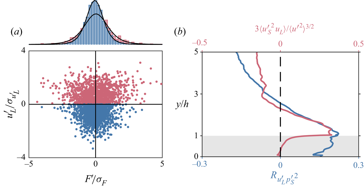
Figure 10(a) shows a distribution plot of the data, with the force acting on the target obstacle  $F'$ along the horizontal axis and the large-scale streamwise velocity fluctuations
 $u'_L$ on the vertical axis. The first striking feature is that high- and low-momentum regions are both likely to produce negative and positive drag fluctuations of comparable intensity. The direct contribution of the large coherent motions to drag fluctuations is associated with quadrants 2 and 4 – when
 $u'_L>0$ then
 $\partial p/\partial x>0$, yielding
 $F'<0$ (and vice versa) – but, thus far, the current data seem to suggest that its significance is not as important as the contribution of more compact, isotropic structures. These are possibly related with sweeps and ejections of the order of the canopy scale that contribute to the Reynolds shear stresses and finer vortical motions populating the shear layer. The symmetry of the scattered data along the vertical axis supports this conclusion, because it suggests that the nature of the dominant processes driving positive- and negative-drag events are essentially the same.
Effect of AM. (a) Scatter plot of the data with force fluctuations  $F'$ on the
 $x$-axis and the large-scale component of the streamwise velocity
 $u'_L$ on the
 $y$-axis. Above are the PDFs of the force conditionally averaged on a high (red) and low (blue) momentum LSM. (b) Wall-normal distributions of the correlation coefficient
 $R_{u'_L {p'_S}^2}$ on the bottom axis (blue) and the cross-term
 $\langle {u'_s}^2 u'_L \rangle$ of the scale-decomposed skewness factor on the top axis (red).

Although there is a weak correlation between  $u'_L$ and
 $F'$, the most extreme excursions of the force appear to be preferentially aligned with high-momentum large-scale events. This is clearly evident by comparing the conditional PDF of the force in the presence of a negative or positive LSM,
 $f_F(F'\mid u'_L <0)$ and
 $f_F(F'\mid u'_L >0)$, respectively. The first distribution is visibly narrower, specifically, force fluctuations greater than
 $\sigma _F$ in absolute terms are nearly
 $30\,\%$ more likely to be associated with a positive large-scale event. The existence of an interaction mechanism of AM could explain this observation, whereby the local pressure fluctuations induced by the small-scale dynamics would be amplified or attenuated along with the turbulent kinetic energy. We test this hypothesis first, by decomposing the fluctuating pressure field into large and small scales using POD, in the same manner as detailed in § 3 for the streamwise velocity component. Accordingly, the pressure signal of the small scales
 $p'_S = p' - p'_L$. The pressure signal from the largest scales
 $p'_L$ is approximated by the linear combination of the first two POD modes, because the second pressure mode shape
 $\phi _B^{(2)}$ was found to match the first EPOD mode shape
 $\phi _e^{(1)}$, which is presumably the footprint of the large-scale velocity structures (refer to figure 8). Second, following an equivalent approach to that outlined by Mathis et al. (Reference Mathis, Marusic, Hutchins and Sreenivasan2011b), a measure of the modulation effect is obtained by computing the correlation coefficient
 \begin{equation} R_{u'_L {p'_S}^2}(\boldsymbol{x}) = \langle u'_L(\boldsymbol{x},t){p'_S}^2(\boldsymbol{x},t) \rangle /(\sigma_{u'_L}(\boldsymbol{x})\sigma_{{p'_S}^2}(\boldsymbol{x})). \end{equation}
In contrast to the filtered envelope of the small-scale pressure fluctuations,  ${p'}_S^2$ accounts not only for the potential large-scale modulation but also for the small-scale variance. Although far from ideal, a more precise description of this interaction may only be achieved with synchronous, time-resolved measurements of the velocity and pressure fields that are not yet available. The wall-normal evolution of the correlation function is shown in figure 10(b), overlaid by the cross-term
 $\langle {u'_s}^2 u'_L \rangle$ of the scale-decomposed skewness factor. The correlation value marginally increases across the canopy, reaching a positive peak around the shear-layer interface. It then monotonically decreases with height and becomes negative in the outer region of the boundary layer. Remarkably,
 $R_{u'_L {p'_S}^2}$ closely traces the evolution of the cross-term
 $\langle {u'_s}^2 u'_L \rangle$, exhibiting a peak and zero crossing at the same locations.
The qualitative similarity between the profiles indicates that the AM of the small-scale pressure fluctuations and turbulent kinetic energy are fundamentally coupled around the near-canopy region. Below the shear layer, however, the correlation function is non-zero despite the sheltering it provides from the flow above. This is an important aspect because it illustrates how the high-frequency component of the drag force may likely be modulated. The fact that the shear-layer interface does not prevent AM of the small-scale pressure signal, as it does with the turbulent kinetic energy, is related to the non-local nature of the pressure field (Tsinober Reference Tsinober2001), which may depend on the flow dynamics far from the point under consideration. Pressure fluctuations within the canopy are then subject to the direct influence of the overlying turbulent motions and, as a result, so are the forces acting on the windward and leeward sides of the roughness obstacles.
6. Further discussion and conclusion
Velocity maps of the boundary-layer flow over a staggered-cube array and the underlying pressure field were used to investigate the turbulent mechanisms responsible for surface drag generation. Statistics of the force acting on a target roughness obstacle exhibit extreme excursions from the mean value, with recurring thrust-producing events. They additionally show a strong correlation between the windward- and leeward-force components, which implies the existence of a coupling mechanism driven by a large-scale, advecting pressure wave, whose direct contribution to the drag force fluctuations is not as significant as that of less intense, anti-signed events (i.e.  $F'_w>0 \cap F'_l<0$).
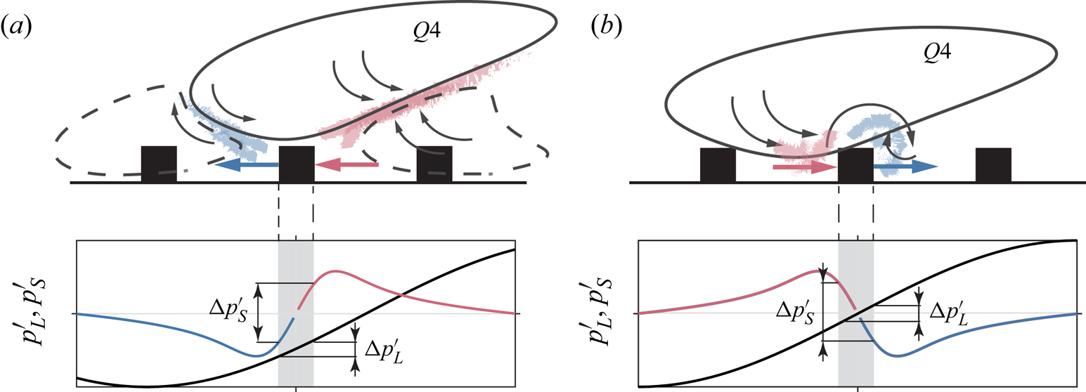
Conditional analyses were performed to explain these observations. The results are schematically summarised in figure 11. We identified distinct flow patterns responsible for positive- and negative-drag fluctuations. The former is dominated by the presence of a forward-leaning high-momentum region impinging on the windward side of the cube, leading to a local increase in pressure. In contrast, the latter features an inclined shear layer squeezed in between an upstream, high-speed sweep, and a downstream, low-speed ejection. This is often referred to as a bursting event, and in agreement with the current results, it has been shown to have a broad effect on the pressure field of smooth-wall boundary layers (Thomas & Bull Reference Thomas and Bull1983). Force fluctuations may thus arise not only from momentum-driven processes, but also due to violent inward–outward flow interactions high above the canopy. It is observed that high-momentum regions, in particular  $Q4$ events, generally experience an adverse pressure gradient, with prevailing negative and positive fluctuations upstream and downstream from the locus of the coherent motion, respectively. Conversely, low-momentum regions, or
 $Q2$ events, are associated with favourable pressure gradients. The cross-over point in pressure is approximately aligned with the local extrema of the velocity fluctuations (i.e. a local maximum/minimum for high-/low-momentum regions). So an increased pressure region may be associated with flow features that exhibit a local streamwise deceleration, and conversely a decreased pressure region is associated with a local acceleration.
Idealised thrust (a) and drag (b) producing events in the presence of a high-momentum region. Brush strokes indicate a local increase (shades of red) or decrease (shades of blue) in static pressure. Represented below is the pressure wave induced by the passage of the LSM (black line) and the small-scale pressure signal for negative (blue) and positive (red) events. The adverse pressure gradient affects the flow field over a wide region, so its direct contribution to the total force acting on the roughness elements  ${\rm \Delta} p'_{L}$ is not as important as that of intermediate and small-scale dynamics
 ${\rm \Delta} p'_{S}$.

The pressure signature of the large scales is consistent with the hypothesis of an advecting pressure wave inducing extreme force fluctuations on opposite sides of the roughness obstacles. A combined analysis of the POD modes of velocity and corresponding EPOD modes of pressure confirmed that large-scale structures are the greatest contributor to the total pressure fluctuations. Yet, their direct impact on surface drag appears to be mitigated by the relative size of the roughness obstacles  $h/L_x$, which is considerably smaller in comparison. We additionally found convincing evidence that the small-scale turbulent pressure fluctuations are influenced by the passage of outer-layer large-scale events through a mechanism that could be AM. Notably, the criteria used to quantify this interaction is non-negligible within the canopy, so it seems that the high-frequency force fluctuations are implicitly modulated. This conclusion is in agreement with recent findings of Cameron et al. (Reference Cameron, Nikora and Marusic2019), who investigated the velocity–drag interrelation on bed-particle flows.
In the same manner as in smooth-wall boundary layers, surface drag arises over rough walls from a superposition of events at different scales interacting with each other. This behaviour is intrinsic to all high Reynolds number wall-bounded turbulence (Marusic et al. Reference Marusic, Mathis and Hutchins2010), but despite their common features, the mechanisms responsible for drag generation are fundamentally different as a result of the surface geometry. For example, we find that positive and negative fluctuations of the force acting on a roughness obstacle are equally likely to occur irrespective of the large-scale signal, whereas over smooth walls the latter is correlated with extreme shear-stress events (Hutchins et al. Reference Hutchins, Monty, Ganapathisubramani, Ng and Marusic2011). In this work, the influence of the large scales on surface drag only becomes apparent by examining the magnitude of the force fluctuations, which are amplified and attenuated in the presence of high- and low-momentum regions, respectively. To achieve a more precise description of this interaction, simultaneous time-resolved pressure and velocity information would be required and should be the topic of future studies.
Acknowledgements
This work was financially supported by the Engineering and Physical Sciences Research Council (EPSRC) through grants EP/P009638/1 and EP/P021476/1. Any relevant data produced in this study are openly available on the research data archive of the University of Southampton at https://doi.org/10.5258/SOTON/D1633.
Declaration of interests
The authors report no conflict of interest.