2. Governing equations and numerical methods

We consider a flow domain bounded by a hot plate at the bottom and a cold plate at the top, with the two plates being perpendicular to gravity and separated by a distance $H$ . Two porous layers with height $H_m$ are located adjacent to the top and bottom plates. The porous layers are saturated with the same working fluid as that in the pure fluid layer. We choose the fluid state at the top plate as the reference state with density $\rho _0$ and temperature $T_0$ . The bottom plate has a higher temperature of $T_0+\Delta _T$ . The linear equation of state is employed as $\rho = -\beta T$ , with $\rho$ and $T$ being the deviation from the corresponding values at reference state, and $\beta$ the positive thermal expansion coefficient. The schematic illustration of the flow configuration is shown in figure 1. To balance enhanced vertical heat conduction within the porous layer and fluid exchange at the interface, while ensuring continuity of the effective thermal diffusivity, the porosity $\phi _e$ is set to vary linearly from the boundary plate to the interface with the middle fluid layer as

(2.1) \begin{align} \phi _e =\left \{ \begin{aligned} & z/H_m, && 0 \leqslant z\lt H_m, \\ & 1, && H_m\leqslant z\leqslant H-H_m, \\ & (H-z)/H_m, && H-H_m\lt z \leqslant H. \\ \end{aligned}\right . \end{align}

In the numerical implementation, a cutoff $\phi _{\textit{cr}}=0.01$ is applied such that $\phi _e \geqslant \phi _{\textit{cr}}$ everywhere to avoid singularities in the momentum equation. The justification for this value, based on the negligible flow observed in regions with $\phi _e\lt 0.01$ even under strong convection, is provided in Supplementary Material § 5 is available at https://doi.org/10.1017/jfm.2026.11127.

To model the incompressible flow and heat transfer, we adopt the one-domain approach where a unified Darcy–Brinkman equation describes both the porous regions and the fluid motions (Reun & Hewitt Reference Reun and Hewitt2021). We choose the characteristic scale for length as $H$ , that for temperature anomaly as $\Delta _T$ and that for velocity as $U_{\kern-1.5pt f}=\sqrt {g\beta \Delta _TH\,}$ where $g$ is the gravitational acceleration. Then, under the Oberbeck–Boussinesq approximation, the non-dimensional governing equations are

(2.2a) \begin{align} &\boldsymbol{\nabla }\boldsymbol{\cdot }\boldsymbol{u} = 0, \\[-12pt] \nonumber \end{align}

(2.2b) \begin{align} &\partial _{t}\boldsymbol{u}+\boldsymbol{u}\boldsymbol{\cdot }\boldsymbol{\nabla }\left (\frac {\boldsymbol{u}}{\phi _e}\right )= -\phi _e\boldsymbol{\nabla }p +\sqrt {\frac {\textit{Pr}}{\textit{Ra}}}\left [{\nabla} ^{2}\boldsymbol{u}-\frac {\phi _e}{\textit{Da}}\boldsymbol{u}\right ] +\phi _e\theta \boldsymbol{e}_z, \\[-12pt] \nonumber \end{align}

(2.2c) \begin{align} &\partial _{t}{\theta } +\boldsymbol{u}\boldsymbol{\cdot }\boldsymbol{\nabla }{\theta } =\frac {1}{\sqrt {\textit{Pr}{\textit{Ra}}}}\boldsymbol{\nabla }\boldsymbol{\cdot }\left (\alpha _m\boldsymbol{\nabla }\theta \right ). \\[9pt] \nonumber \end{align}

Here, $\boldsymbol{u}$ is velocity, $p$ is pressure and $\theta =(T-T_0)/\Delta _T$ is temperature, all in their non-dimensional forms. The effective thermal diffusivity ratio $\alpha _m$ is calculated as $\alpha _m=\phi _e+\alpha _\kappa (1-\phi _e)$ and $\alpha _\kappa =\kappa _p/\kappa _{\kern-1pt f}$ is the ratio between the thermal diffusivity of porous matrix material and that of fluid. The other control parameters include the Prandtl number, the Rayleigh number and the Darcy number, which are respectively defined as

(2.3) \begin{align} \textit{Pr} = \frac {\nu }{\kappa _{\kern-1pt f}}, \quad {Ra} = \frac {g\beta \Delta _T H^3}{\kappa _{\kern-1pt f{\kern-1pt}}\nu }, \quad Da = \frac {K}{H^2}. \end{align}

For the permeability $K$ we adopt the Kozeny–Carman relation (Paoli et al. Reference Paoli, Howland, Verzicco and Lohse2024)

(2.4) \begin{align} K=\frac {D^2}{180}\frac {\phi _e^3}{{\left (1-\phi _e\right )}^2}, \end{align}

where $D$ is the diameter of solid obstacles in the porous matrix. Regarding the limit $\phi _e \to 1$ : although the Kozeny–Carman expression diverges, the relevant quantity in the momentum (2.2b ) is the inverse permeability $1/K(\phi _e)$ . As $\phi _e$ approaches unity, $1/K(\phi _e)$ smoothly tends to zero, thereby eliminating the Darcy drag term and naturally recovering the standard Navier–Stokes equations for a pure fluid. Consequently, no additional numerical regularisation is needed near $\phi _e = 1$ . The Rayleigh number for the middle fluid layer can be calculated as $ \textit{Ra}_b = \textit{Ra} (1-2h_m )^3$ with $h_m=H_m/H$ . As shown in § 3 of the Supplementary Material, the temperature gradient within each porous layer is extremely small when $\alpha _\kappa \gg 1$ . Hence, we assume the temperature difference across one porous layer is negligible.

Figure 1.

Schematic illustration of system configuration and boundary conditions.

The non-dimensional governing equation, (2.2), is numerically solved by using our in-house code, which is built on the extensively used code for RBC and other wall-bounded turbulence (Verzicco & Orlandi Reference Verzicco and Orlandi1996; Ostilla-Mónico et al. Reference Ostilla-Mónico, Yang, Poel, Lohse and Verzicco2015). The original code is modified to be able to handle the Darcy–Brinkman equation with inhomogeneous permeability and porosity, and the temperature equation with non-uniform thermal diffusivity. The code employs a second-order finite difference scheme for spatial discretisation and the fractional time-step method. The nonlinear terms are treated explicitly with an Adams–Bashforth type of scheme and the diffusion terms semi-implicitly with a Crank–Nicholson type of scheme. A second-order Runge–Kutta type of scheme is used for the temporal integration. Further details on the numerical implementation, validation and convergence tests can be found in our recent work (Guo & Yang Reference Guo and Yang2025).

In all simulations we set the domain height at $H=120\,\mathrm{mm}$ and the diameter of the solid obstacle in the porous matrix at $D=1\,\mathrm{mm}$ . This combination of a small obstacle size and the high solid thermal conductivity used in our study ( $\alpha _\kappa =10^3$ ) ensures that, even when the entire domain is occupied by porous layers ( $h_m=0.5$ ), the effective Rayleigh number within the porous medium remains far below the critical threshold for Rayleigh–Darcy convection. Consequently, all flow observed in our simulations results from inertial penetration driven by convection in the adjacent free-fluid layer, rather than from spontaneous buoyancy-driven instability within the porous medium itself. Three groups of simulations were carried out to reveal the influences of different control parameters. For the first group we fix $ \textit{Pr}=1$ and $\alpha _\kappa =10^3$ , and systematically vary $ \textit{Ra} $ and $h_m$ . For the other two groups we fix $ \textit{Ra}=10^7$ and $h_m=0.2$ , and change $ \textit{Pr} $ or $\alpha _\kappa$ . Details of all simulations are summarised in the Supplementary Materials, along with the code validation and grid-convergence test.

3. Heat-flux enhancement and physical mechanisms

We first compare the flow structures for two cases with $h_m=0.02$ and $0.2$ in figure 2. The two cases share the same parameters as $ \textit{Ra}=10^8$ , $ \textit{Pr}=1$ and $\alpha _m=10^3$ . The flow field of the case with $h_m=0.02$ is very close to that of traditional RBC without a porous layer. However, with the same Rayleigh number, the flow motions of the case with $h_m=0.2$ are much stronger due to the existence of the thick porous layer. The plumes and the resulting large-scale circulations are significantly intensified. In particular, it can be clearly noticed that, within the porous layer, there exists spatial variation of temperature, which is caused by the convection flows inside the porous regions.

Figure 2.

Volume rendering of the temperature field for $ \textit{Ra}=10^8$ , $ \textit{Pr}=1$ and $\alpha _m=10^3$ . Panels show (a) $h_m=0.02$ , (b) $h_m=0.2$ .

To illustrate the coupling of the flow motions in the fluid layer and those in the porous layer, the instantaneous and temporally averaged flow fields on a vertical plane are shown in figure 3 for the temperature contours and in-plane streamlines. It is clear that the streamlines are continuous across the interfaces between the fluid layer and porous layers. In particular, in the impacting or ejecting regions the instantaneous streamlines travel through the interfaces nearly perpendicularly. For the temporally averaged field, the unified large-scale convection rolls cover both the fluid and porous layers, which is very similar to those reported in Zou & Yang (Reference Zou and Yang2021). The strong coupling of momentum field between the fluid and porous layers greatly enhances the heat transfer across the interface, and causes the inhomogeneous temperature variation inside the porous layers.

Figure 3.

(a) Instantaneous and (b) temporally averaged flow field on a vertical slice is shown for $ \textit{Ra}=10^8$ , $ \textit{Pr}=1$ , $h_m=0.2$ and $\alpha _m=10^3$ by the streamlines of in-plane velocity and the contours of the temperature field.

To measure the transport properties of the fluid layer between the two porous layers, we define the Nusselt number and the Reynolds number as

(3.1) \begin{align} \textit{Nu}_b = \frac {{\left \langle U_z T\right \rangle }_{\textit{bulk}}-\kappa _{\kern-1pt f}\partial _z{\left \langle T\right \rangle }_{\textit{bulk}}}{\kappa _{\kern-1pt f}\Delta _T{(H-2H_m)}^{-1}}, \quad \textit{Re}_b = \frac {U_{\textit{rms}}\left (H-2H_m\right )}{\nu }, \end{align}

where $\left \langle \boldsymbol{\cdot }\right \rangle _{ {bulk}}$ denotes the average over the fluid layer and time. Here, $U_z$ is the dimensional velocity in the vertical direction, and $U_{\textit{rms}}$ is the root-mean-square value of velocity magnitude calculated over the fluid layer. Strictly speaking, the Nusselt number should be defined by using the conductive temperature difference $\Delta _T^{\kern-2pt f}$ across the fluid layer. In practice, however, we adopt the total temperature difference $\Delta _T$ together with the height of the fluid layer, because the temperature drop across the porous layer is relatively small. For the case $\alpha _\kappa =10^3$ considered here, the relative difference between $\Delta _T$ and $\Delta _T^{\kern-2pt f}$ is less than $0.5\,\%$ (see Supplementary Material § 3). When $H_m$ reduces to zero, the above definitions recover those for RBC.

Figure 4 presents the dependence of $ \textit{Nu}_b$ and $ \textit{Re}_b$ on $ \textit{Ra}_b$ for fixed $ \textit{Pr}=1$ and $\alpha _\kappa =10^3$ . The same data are plotted in both the original form and the compensated form, and are compared with those of traditional RBC with both no-slip and free-slip boundary conditions. Also four groups of simulations were run with $h_m$ increasing from $0.02$ to $0.2$ . Even for the thinnest porous layer with $h_m=0.02$ , as shown in panel (a), a noticeable increase in $ \textit{Nu}_b$ can be observed but the scaling relation with $ \textit{Ra}_b$ does not change. As $h_m$ becomes larger, the enhancement of $ \textit{Nu}_b$ also becomes stronger. In particular, when $h_m$ is large enough, the enhancement of $ \textit{Nu}_b$ is bigger at higher $ \textit{Ra}_b$ than that at lower $ \textit{Ra}_b$ . For example, the highest increase in $ \textit{Nu}_b$ is obtained for $h_m=0.2$ and the highest Rayleigh number $ \textit{Ra}=10^8$ or $ \textit{Ra}_b=2.16\times 10^7$ . The increment is approximately $400\,\%$ compared with RBC at the same Rayleigh number. As a result, for $h_m=0.2$ , the scaling relation between $ \textit{Nu}_b$ and $ \textit{Ra}_b$ is different for $ \textit{Ra}_b\le 2.16\times 10^6$ and $ \textit{Ra}_b\ge 2.16\times 10^6$ in the current simulations. Meanwhile, the influence of the porous layers on the behaviour of $ \textit{Re}_b$ is totally different from that on $ \textit{Nu}_b$ . By introducing porous layers, the Reynolds number $ \textit{Re}_b$ is also increased compared with the RBC with the same $ \textit{Ra}_b$ , but not as much as that of the Nusselt number $ \textit{Nu}_b$ . Unlike the Nusselt number $ \textit{Nu}_b$ , for a given $h_m$ , $ \textit{Re}_b$ follows a single power-law scaling with $ \textit{Ra}_b$ and the exponent increases slightly as the porous layer becomes thicker.

Figure 4.

Dependence of $ \textit{Nu}_b$ and $ \textit{Re}_b$ on $ \textit{Ra}_b$ for different heights $h_m$ of the porous layer and fixed $ \textit{Pr}=1$ and $\alpha _\kappa =10^3$ . Solid symbols represent our data, including the case of a uniform porosity of $\phi _e=0.5$ (blue pentagrams), while open symbols represent the reference data from other studies. The red circles and the red pentagrams represent, respectively, the results of RBC with no-slip boundaries and those of the homogeneous temperature layers from Zou & Yang (Reference Zou and Yang2021). The blue squares to represent RBC with a free-slip boundary (Huang & He Reference Huang and He2022). (a,b) The original values and the corresponding power-law scalings. (c,d) The compensated plots of the same data.

To reveal the physical mechanism of the heat-flux enhancement more clearly, we plot the horizontally and temporally averaged profiles of key flow variables in figure 5 for the cases with increasing $ \textit{Ra} $ and fixed $ \textit{Pr}=1$ and $h_m=0.2$ . For the two smaller Rayleigh numbers, the averaged temperature is nearly constant within the porous layers and equal to the corresponding values at the adjacent boundaries. The temperature fluctuation and the velocity are almost zero inside the porous layer. As the Rayleigh number increases, noticeable flow motions develop within the porous layer and close to the interface with the fluid layer. Therefore, the mean temperature deviates from the corresponding boundary value and exhibits spatial and temporal fluctuations; see the mean profiles in figures 5(a) and 5(b) for cases with $ \textit{Ra}=10^7$ and $10^8$ , respectively. As a result, the convective flux is already quite strong at the interface, see figure 5(e). Here the convective flux is calculated as $\overline {q}_c=\langle u_z'T'\rangle /[\kappa _{\kern-1pt f}\Delta _T{(H-2H_m)}^{-1}]$ . For completeness, the profiles of conductive flux, which is calculated as $\overline {q_d}=\langle \alpha _m\kappa _{\kern-1pt f}\partial _z T\rangle /[\kappa _{\kern-1pt f}\Delta _T{(H-2H_m)}^{-1}]$ , are shown in figure 5(f). As $ \textit{Ra}_b$ increases, the thickness of the region where $\overline {q}_c$ is stronger than $\overline {q}_d$ becomes larger.

Figure 5.

Profiles of (a) the mean temperature $\overline {\theta }$ , (b–d) the standard deviations of temperature $\theta '$ , horizontal velocity $u_x'$ and vertical velocity $u_z'$ , respectively, and (e–f) the convective and conductive heat flux $\overline {q_c}$ and $\overline {q_d}$ . The shaded regions indicate the porous layers. Different lines correspond to different Rayleigh numbers, $ \textit{Ra} $ , as indicated in the legend above the panels. For all cases $ \textit{Pr}=1$ and $h_m=0.2$ .

As shown in figures 4(a) and 4(c), the heat flux is consistently enhanced for the four cases shown in figure 5, even though the flow motions are only visible inside the porous layer for large Rayleigh numbers. To clarify the origin of the heat-flux enhancement, we calculate the averaged convective and conductive fluxes of the fluid side at the interface, which are plotted in figure 6(a) versus the Rayleigh number for the cases with $ \textit{Pr}=1$ and $h_m=0.2$ . The summation of the two components gives the total Nusselt number. For $ \textit{Ra}_b\le 2.16\times 10^6$ , the conductive flux $\overline {q}_d$ is considerably larger than the convective flux $\overline {q}_c$ . For $ \textit{Ra}_b=6.48\times 10^6$ , the two fluxes are almost equal to each other. While for the largest $ \textit{Ra}_b=2.16\times 10^7$ , the convective flux becomes much larger than the conductive flux.

Figure 6.

(a) The averaged and non-dimensionalised conductive and convective fluxes at the fluid side of interface versus the Rayleigh number. (b) The thicknesses of thermal and momentum boundary layers adjacent to the interface versus the Rayleigh number. (c) The root mean square of vertical velocity at the interface versus the Rayleigh number. For all cases, $ \textit{Pr}=1$ and $h_m=0.2$ . The open circles in (a) and (b) represent the data of RBC from Zou & Yang (Reference Zou and Yang2021).

For comparison, the Nusselt number of RBC is also included in figure 6(a). It is immediately clear that the heat-flux enhancement comes from the conductive component at low Rayleigh number, and from the convective component for large Rayleigh number. At small Rayleigh number, as shown by the profiles in figure 5, the porous layer has nearly constant mean temperature and no flow motions. Due to the high diffusivity of porous matrix, the fluid exchanges heat over the entire porous layer. Moreover, the porosity at the interface reduces the friction of horizontal flow motions, resulting in stronger convection rolls and thinner boundary layers at the interface than those in RBC, as indicated by figure 6(b). When the Rayleigh number is large enough, for the given $h_m=0.2$ , the convection motions inside the porous medium is strong enough to generate large permeable velocity and convective flux across the interface. Figure 6(c) indicates the vertical velocity fluctuation at the interface, measured by the root mean square of vertical velocity $u'_z$ , increases with the Rayleigh number according to the power-law scaling of $u'_z\sim {Ra}_b^{0.41}$ . This is different compared with the convection system with permeable walls studied by Kawano et al. (Reference Kawano, Motoki, Shimizu and Kawahara2021), where the permeable velocity is assumed to be proportional to the vertical pressure gradient at the wall. Kawano et al. (Reference Kawano, Motoki, Shimizu and Kawahara2021) found that the fluctuation of the permeable velocity at the walls decreases initially with $ \textit{Ra} $ and then saturates, and $Nu$ scales as $ \textit{Ra}^{1/2}$ when $ \textit{Ra} $ is large enough. Here, the permeable velocity at the interface increases with $ \textit{Ra} $ and the resulting scaling exponent for $Nu$ versus $ \textit{Ra} $ is higher than $1/2$ , see figure 4(a).

We now can draw a general picture for heat-flux enhancement. Although $ \textit{Nu}_b$ constantly increases over all $ \textit{Ra}_b$ explored here when the porous layer is introduced, the different scaling behaviours at small and large $ \textit{Ra}_b$ imply different mechanisms for enhancements. Taking $h_m=0.2$ for example, the exponent of power-law scaling between $ \textit{Nu}_b$ and $ \textit{Ra}_b$ is approximately 0.37 when $ \textit{Ra}_b\lesssim 2.16\times 10^6$ , which is only slightly larger than that for RBC. As shown in figure 4(c), for $ \textit{Ra}_b \lesssim 2.16\times 10^6$ the Nusselt number $ \textit{Nu}_b$ closely follows the trend of $ \textit{Nu}_b$ of RBC with a free-slip boundary. That is, the high-porosity region near the fluid–porous-medium interface generates an effective free-slip boundary. In contrast, for $ \textit{Ra}_b\gtrsim 2.16\times 10^6$ , $ \textit{Nu}_b$ increases more rapidly with $ \textit{Ra}_b$ . The linear fitting gives an exponent of $0.78$ for the power-law scaling between $ \textit{Nu}_b$ and $ \textit{Ra}_b$ . This exponent is even larger than the value of $1/2$ for the ultimate scaling.

The rapid increase of $ \textit{Nu}_b$ at large $ \textit{Ra}_b$ is remarkable in the sense that it exceeds the ultimate scaling. However, quantitative comparison indicates that the absolute value of $ \textit{Nu}_b$ is still smaller than that with homogeneous thermal layer at the same $ \textit{Ra}_b$ in Zou & Yang (Reference Zou and Yang2021). In the work of Zou & Yang (Reference Zou and Yang2021) the homogeneous thermal layer acts as a porous layer with infinite thermal conductivity and uniform porosity of $\phi _e=1$ . The increase of $ \textit{Nu}_b$ as $ \textit{Ra}_b$ becomes larger is solely caused by the strengthening of turbulent motions. In the current system with inhomogeneous porous layers, at $ \textit{Ra}_b$ becomes larger, two effects contribute to the heat-flux enhancement. The first one is the enhancement of turbulent motions. This includes the turbulent motions inside the fluid layer, as demonstrated by the increase of $ \textit{Re}_b$ in figure 4(b). Also the convection motions inside the porous layer are stronger for higher $ \textit{Ra} $ , as shown by the profiles in figure 5. The other effect is the penetration of convection region from the interface towards the solid boundary inside the porous layer as $ \textit{Ra}_b$ increases, which promotes the fluid exchange across the interface and increases the global heat flux. Such process can be inferred from the mean profiles shown in figure 5. As $ \textit{Ra} $ increases, in the porous layer and close to the interface, the region where the temperature and velocity fluctuations are not zero becomes thicker, indicating the expansion of the convection zone.

From figures 4(a) and 4(b) one notices that the heat-flux enhancement of the current system is much weaker than that of the homogeneous layer used in Zou & Yang (Reference Zou and Yang2021). This is reasonable since the homogeneous layers in Zou & Yang (Reference Zou and Yang2021) can be viewed as a porous layer with extremely large thermal conductivity and a porosity of $\phi _e=1$ . That is, the heat exchange with the fluid is very fast while no extra drag force is exerted on fluid motions within the homogeneous layers. Then it is natural to ask whether the large exponent can persist for even larger $ \textit{Ra}_b$ or will it eventually decrease to a smaller value, as the second effect may saturate when the convection region occupies the whole porous layer. This requires investigation at much larger $ \textit{Ra}_b$ .

Next, we examine the influences of $ \textit{Pr} $ and $\alpha _\kappa$ , which are shown in figure 7 for fixed $ \textit{Ra}=10^7$ and $h_m=0.2$ . When changing the Prandtl number of the fluid, we fixed $\alpha _\kappa =10^3$ , so that the thermal diffusivity is always much larger than that of the fluid. Figures 7(a) and 7(b) present the influence of the Prandtl number on heat and momentum transport in our composite system. For reference, the dependence of $ \textit{Nu}_b$ on $ \textit{Pr} $ for the RBC flows and those for homogeneous temperature layers are also shown for $ \textit{Ra}=3\times 10^6$ , with the data adopted from Zou & Yang (Reference Zou and Yang2021). The figures reveal that, although the Nusselt number is greatly enhanced and the Reynolds number is only slightly increased, the overall trends of $ \textit{Nu}_b$ and $ \textit{Re}_b$ are similar to those of RBC, but much smaller than those of cases with homogeneous temperature layers. Meanwhile, figures 7(c) and 7(d) indicate that both $ \textit{Nu}_b$ and $ \textit{Re}_b$ increase with $\alpha _\kappa$ . And more importantly, the enhancement of transport can only be obtained when $\alpha _\kappa$ is large enough, such as two orders of magnitude larger than that of the fluid for the current case. This is expected since only when the heat diffuses much faster along the porous matrix is the effective thermal diffusivity $\alpha _m$ of the saturated porous layer of fluid considerably greater than that of pure fluid.

Figure 7.

The dependence of $ \textit{Nu}_b$ and $ \textit{Re}_b$ on (a, b) $ \textit{Pr} $ and (c, d) $\alpha _\kappa$ for fixed $ \textit{Ra}=10^7$ (or $ \textit{Ra}_b=2.16\times 10^6$ ) and $h_m=0.2$ . For (a) and (b) $\alpha _\kappa =10^3$ , while for (c) and (d) $ \textit{Pr}=1$ . In (a) and (b), the open circles and open squares respectively represent the RBC and the homogeneous temperature results at $ \textit{Ra}=3\times 10^6$ from Zou & Yang (Reference Zou and Yang2021). The horizontal lines in (c) and (d) mark the corresponding values of RBC.

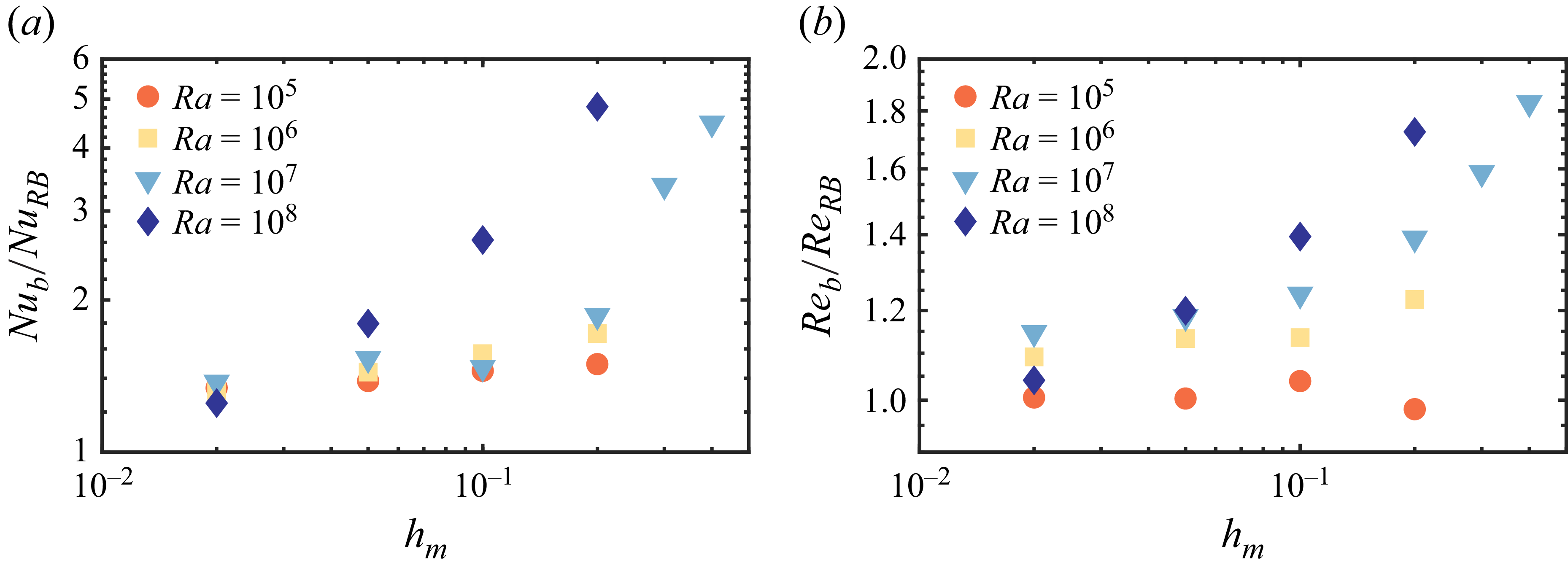
We now discuss the influences of the porous layer properties on the heat-transfer enhancement. We first look at the influence the porous layer thickness $h_m$ . Figure 8 shows the increase of $ \textit{Nu}_b$ and $ \textit{Re}_b$ versus $h_m$ by the ratio of them to the corresponding values of RBC at the same $ \textit{Ra}_b$ corresponding to the specific $h_m$ . Note that, for fixed $ \textit{Ra} $ , $ \textit{Ra}_b$ decreases as $h_m$ becomes larger. At small $h_m$ , both $Nu$ and $Rey$ are close to the corresponding RBC values. It is noticeable that heat-flux and flow motion enhancement happens when $h_m$ is large enough. Moreover, the enhancement sets in at smaller $h_m$ for higher $ \textit{Ra} $ .

Figure 8.

The increases of (a) $ \textit{Nu}_b$ and (b) $ \textit{Re}_b$ versus $h_m$ for different Rayleigh numbers $ \textit{Ra} $ and fixed $ \textit{Pr}=1$ and $\alpha _\kappa =10^3$ . The values are normalised by those of RBC at the same $ \textit{Ra}_b$ .

Finally, to provide some insights into the necessity of inhomogeneous porosity to the heat-flux enhancement, an extra case has been simulated with $ \textit{Ra}=10^8$ , $h_m=0.2$ and uniform porosity $\phi _e=0.5$ . Figure 9 depicts both the instantaneous and temporally averaged flow fields on a vertical plane by showing the temperature contours and in-plane streamlines. Compared with the case with a linear porosity profile and mean porosity of $\phi _e=0.5$ shown in figure 3 with the same $ \textit{Ra} $ and $h_m$ , it is clear that the temperature inside the porous layer is more homogeneous for the case with uniform porosity. Moreover, at the interface, most of the streamlines are parallel to the interface in figure 9. Therefore, the fluid exchange across the interface is much weaker when the porous layer is homogeneous with moderate porosity. In other words, the large porosity near the interface is necessary for efficient heat transfer between different layers by momentum coupling, while the small porosity near the solid boundary is necessary for efficient heat transfer from the boundary to inside of the domain. As a result, the case with uniform porosity $\phi _e=0.5$ does not generate heat-flux enhancement, see figure 4.

Figure 9.

(a) Instantaneous and (b) temporally averaged flow field on a vertical slice is shown for $ \textit{Ra}=10^8$ , $ \textit{Pr}=1$ , $h_m=0.2$ and $\alpha _m=10^3$ by the streamlines of in-plane velocity and the contours of temperature field. A uniform porosity of $0.5$ is applied within the porous layers.