Implications
Accurate measurements of methane (CH4) emissions are essential to understand the importance of livestock's contribution to the greenhouse gas issue, and to develop mitigation strategies to improve the environmental sustainability of animal agriculture. These goals will become even more important as animal production escalates to meet global population demands. A clear understanding of the limitations and accuracy of measurement techniques presented in this review is needed to advance our understanding of CH4 emissions from animal agriculture.
Introduction
Animal agriculture production is estimated to account for 8% to 10.8% of the global emissions of greenhouse gases (O'Mara, Reference O'Mara2011). Methane (CH4) is a large component of these emissions where globally the annual emission of ruminant enteric CH4 is 91.9 million tonnes, and CH4 from livestock manure is 11.2 million tonnes (O'Mara, Reference O'Mara2011). The enteric CH4 from ruminants alone is estimated to account for 25% to 40% of the anthropogenic release of CH4 (Clark, Reference Clark2013). It follows that accurate measurement of CH4 emissions from ruminants and livestock manure is necessary to develop best management practices to reduce these CH4 emissions and to ultimately improve the environmental sustainability of the livestock industry. These goals will become even more relevant with the expected expansion of the livestock industry because of increased demand for meat and milk by an escalating human population estimated to reach nine billion by 2050 (Smith et al., Reference Smith, Matino, Cai, Gwary, Janzen, Kumar, McCarl, Ogle, O'Mara, Rice, Scholes, Sirotenko, Howden, McAllister, Pan, Romanenkov, Schneidere and Towprayoon2007). Fundamental to accurate measurement is the need for techniques that give direct measurements of CH4 emissions under a variety of management and environmental conditions.
A variety of CH4 emission techniques for intensive livestock systems have been reviewed in the literature, for example, National Research Council (2003) and McGinn (Reference McGinn2006). The review edited by Makkar and Vercoe (Reference Makkar and Vercoe2007) outlined in a series of chapters in vitro and in vivo techniques, where the latter included the enteric tracer technique (i.e., using an enteric permeation tube containing sulphur hexafluoride (SF6)) as well as the tunnel and chamber methods, but did not cover micrometeorological techniques. Denmead (Reference Denmead2008) discussed the use of chambers (surface) and micrometeorological techniques for CH4 and nitrous oxide sources. A focused review by Harper et al. (Reference Harper, Denmead and Flesch2011) also described a few non-micrometeorological techniques (animal chambers, enteric tracer, external tracer and mass balance) and provided an in-depth description of micrometeorological techniques used to estimate CH4 emissions from livestock. A more recent review of techniques for measuring CH4 emissions from livestock was presented by Storm et al. (Reference Storm, Hellwing, Nielsen and Madsen2012), mostly covering the use of animal chambers, enteric tracer, in vitro and modelling; other techniques are very briefly mentioned including some micrometeorological techniques. This review provides an overview of the micrometeorological techniques, whereas the appropriate reviews mentioned above can provide the details.
The objective of the current review is to build on the previous reviews by focusing on the limitations of specific micrometeorological techniques and their practical application to animal agriculture CH4 emissions. Insights into the accuracy are also investigated by reporting on studies where emissions using different techniques are compared. Finally, a discussion follows on the recent developments in micrometeorological techniques to estimate CH4 emissions from livestock and livestock manure.
General application of micrometeorological techniques
There exists an assortment of micrometeorological techniques for calculating the emission of enteric CH4 from ruminants (Harper et al., 2011) or CH4 directly from livestock manure. These include the flux gradient (FG), eddy covariance (EC), relaxed eddy accumulation (REA), integrated horizontal flux (IHF) and boundary-layer budgeting (BLB). More recent application of dispersion modelling (e.g., backward Lagrangian stochastic model, BLS) has also been used to estimate emissions from ruminants and livestock manure. A widely used BLS technique is the WindTrax model (Thunder Beach Scientific, Nova Scotia, Canada).
All these micrometeorological techniques share the advantage of being non-intrusive, as well as providing near-continuous emissions data. As micrometeorological techniques generally have a large measurement footprint, they can also result in a spatial average of the source strength. However, not all micrometeorological techniques are conducive to measurement situations in animal agriculture, where the source area is small such as manure storage facilities and small pens containing animals.
Some micrometeorological techniques such as the FG and EC techniques are best suited to operate within the fully adjusted internal boundary layer (IBL), where the properties of the air stream, at the measurement height, is in equilibrium with the surface, that is, the vertical flux at the measurement height equals the emission rate from the underlying surface. A simple ‘rule-of-thumb’ is that the fully adjusted IBL roughly increases in height by 1 m for every 100 m distance from the upwind leading edge of the source area (Vesala et al., Reference Vesala, Kljun, Rannik, Rinne, Sogachev, Markkanen, Sabelfelt, Foken and Leclerc2008). Other more detailed relationships exist in defining this boundary layer, for example, as a function of the surface roughness and distance from the leading edge (Munro and Oke, Reference Munro and Oke1975). CH4 concentrations measured by sensors positioned above the fully adjusted IBL do not correspond with the surface emissions. Where the CH4 source area is small such that the sensor height is above the fully adjusted IBL, it is necessary to calculate a ‘footprint’ of the sensor (the upwind area that influences the sensor's measurements) to determine how much of the source area is seen by the sensor (e.g., as reported by Schuepp et al. Reference Schuepp, Leclerc, MacPhereson and Desjardins1990).
Typically, micrometeorological techniques also assume that the source strength is evenly distributed (spatially homogeneous). Exceptions to this are the modified IHF (modified mass difference (MMD); Harper et al., 2011) technique or when using the BLS (WindTrax) technique where the source location is known and treated as a point source. The need for spatially uniform source strength is more achievable for manure storage facilities such as open pits than for non-confined grazing ruminants. When the enteric CH4 from grazing ruminants is the targeted source, one option is to place global positioning system (GPS) units on the animals and then treat them as point sources (McGinn et al., Reference McGinn, Turner, Tomkins, Charmley, Bishop-Hurley and Chen2011).
It is possible to reduce the impact of assuming even distribution of the source strength when using the BLS technique (Flesch et al., Reference Flesch, Wilson, Harper and Crenna2005). As the distance between the source and location of concentration detection increases, the sensitivity of the calculated emissions to the source distribution decreases. This implies a benefit to having the detection distance away from the source. This principle was demonstrated by McGinn et al. (Reference McGinn, Flesch, Harper and Beauchemin2006) who showed that treating point sources as an area source resulted in smaller error with increased distance between the source and site of CH4 detection. Where a combined emission is from two or more distinct sources (e.g., two barns on a farm), Flesch et al. (2005) reported that positioning the concentration sensor twice the source separation distance downwind gave errors in emissions of <10%. In practice, there is a limitation to the downwind distance, where the concentration dilutes with distance from the source. As a result, while it may be advantageous to have the detector some distance downwind from the source, the source must also be close enough to measure a significant concentration difference from the background concentration. There is also a disadvantage with long distances between the source and sensor in that the operational wind direction ‘window’ narrows with increasing distance.
IHF
The IHF technique is based on the accounting of CH4 entering and leaving a small source (e.g., manure storage pond) via the open air, where the difference is equated to the amount of CH4 emitted by the source. This technique imposes no restriction on the source strength distribution. In this technique, the CH4 emission (Q; g/m2 per s) is calculated as the sum of mean horizontal fluxes accumulated above the source height (z 1; m):
 $$Q\, = \,\frac{1}{x}\mathop{\sum}\limits_{{{z}_1}}^{{{z}_2}} {\,\left[ {\bar{u}\left( {{{{\bar{C}}}_{\rm{d}}}{\rm{ - }}{{{\bar{C}}}_{\rm{u}}}} \right)} \right]} \,{\rm{\rDelta }}z$$
where u is wind speed (m/s), C the concentration (g/m3) and subscripts d and u denote the downwind and upwind locations, respectivelyFootnote 1. The maximum height (z 2) is where the horizontal flux declines to zero (the lowest height where the incoming and outgoing CH4 concentrations become equal), and x is the path distance across the source that the wind follows. With a uniform landscape, it is assumed that the magnitude of the incoming and outgoing u is equal at any given height in equation (1).
The application of the IHF technique is best suited to horizontally uniform surfaces such as a manure storage pond that ensures a smooth C d and u profile. When the IHF technique is applied to source that is not horizontally homogenous, for example, a manure pile or a raised manure storage pond, care must be taken to ensure that the C and u profiles are characterized accurately. This typically requires using at least five sampling heights. Where the height of zero horizontal flux is beyond the highest measurement height, it is possible to account for this by extrapolation. This has been done by regressing C and u against the natural log of the height (ln z) and expressing Q as a function of the regression coefficients (Ryden and McNeill, Reference Ryden and McNeill1984). The IHF-modified version MMD with its more elaborate field requirement does not require that the source strength be spatially evenly distributed. To be independent of wind direction, the MMD requires a horizontal line averaged of concentration along each source perimeter, at several heights on all perimeters (i.e., the face), thereby enclosing the entire source.
Laubach et al. (Reference Laubach, Kelliher, Knight, Clark, Molano and Cavanagh2008) used the IHF technique to determine the enteric emissions from cattle grazing ryegrass in small paddocks. They reported an average enteric CH4 emission of 161 g/animal per day. The IHF technique has also been used to calculate CH4 emissions from open-top tanks containing dairy liquid manure, ranging between 11 (after emptying) and 153 μg/m2 per s (Vanderzaag et al., Reference VanderZaag, Wagner-Riddle, Park and Gordon2011).
In using equation (1), two assumptions are made as outlined by Gao et al. (Reference Gao, Desjardins and Flesch2009). First, it is reasonable to assume that fluctuations in u at one point are the same as fluctuations in wind speed along the entire perimeter when C is a line-average concentration (e.g., using an open-path laser) and u is point measurement along a perimeter. Second, the product of the time-averaged wind speed ( $$$\bar{u}$$$
) and time-averaged concentration (
 $$$\bar{C}$$$
) in equation (1) is a simplification, which should actually be written as the time-averaged product of u and C (
 $$$\overline{{uC}} $$$
). This time-averaging error is often unavoidable owing to instrumentation restrictions (e.g., cup anemometers fail to measure short-term fluctuations). Gao et al. (Reference Gao, Desjardins and Flesch2009) state that this error causes an overestimate (in the MMD technique) of 5% to 20%.
FG
Emissions using the FG technique are calculated as the product of the turbulent (or eddy) diffusivity (K; m2/s) and the vertical concentration gradient (ΔC/Δz; g/m3 per m). The turbulent diffusivity for different properties (e.g., momentum and heat) is assumed to be related, such that it can be determined by combining atmospheric properties. The Schmidt number (Sc), for example, is the ratio of turbulent diffusivity of momentum to mass (Sc = K m/K c). Therefore, determining K m provides an estimate of K c when the value of Sc is knownFootnote 2. The value of K m is calculated (Monteith, Reference Monteith1973) using:
 $${{K}_{\rm{m}}}\, = \,\frac{{k{{u}^\ast} z}}{{{{\phi }_{\rm{m}}}}}$$
where von Karman's constant (k ) relates the size of eddies to height above ground, friction velocity (u*; m/s) is derived from wind statistics measured using a three-dimensional sonic anemometer, z (m) is the measurement height above the surface and φ m a non-dimensional correction for the effect of thermal stability on the wind profile. This stability correction is calculated as a function of the atmospheric stability as reflected in the Monin–Obukhov parameter (L; m). The FG emission (Q in g/m2 per s) is then given as:
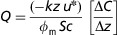 $$Q = \frac{{({\rm{ - }}kz\,{{u}^\ast} )}}{{{{\phi }_{\rm{m}}}\,Sc}}\,\left[ {\frac{{{\rm{\rDelta }}C}}{{{\rm{\rDelta }}z}}} \right]$$
The FG technique was first applied to livestock where enteric CH4 from grazing sheep was measured by Judd et al. (Reference Judd, Kelliher, Ulyatt, Lassey, Tate, Shelton, Harvey and Walker1999). Since then, this technique has also been applied to grazing cattle (Laubach et al., Reference Laubach, Kelliher, Knight, Clark, Molano and Cavanagh2008). Like other micrometeorological techniques, FG is best suited to operate in the fully adjusted IBL; else a footprint model (Vesala et al., Reference Vesala, Kljun, Rannik, Rinne, Sogachev, Markkanen, Sabelfelt, Foken and Leclerc2008) must be used to gauge the influence of the source configuration on the calculated emission (see the discussion below).
EC
The EC technique is based on monitoring the vertical flux of a gas at a point above the source area. For a horizontally extensive source, the surface emission Q (g/m2 per s) is taken as equal to the vertical flux at the measurement point, and is determined as the product of the instantaneous deviation from the mean vertical wind speed (w′; m/s) and the instantaneous deviation from the mean CH4 concentration (C′; g/m3):
 $$Q = \overline{{w^{\prime}\,C^{\prime}}} $$
where the overbar indicates that the cross product is averaged, usually over a 10 to 30 min interval. This technique requires sensors with very fast response times to measure w and C, in the order of 10 times a second (10 Hz). A three-dimensional sonic anemometer is generally used to measure w. Post-measurement corrections (coordinate rotations) are needed to ensure the mean w is zero.
When applying the EC technique, consideration must be made for the characteristics of the upwind source area. Where the upwind source is extensive and homogeneous, the location of the EC detectors should be at a height within the fully adjusted IBL (reflective of the surface emission). Where the source is not extensive (finite) and/or not evenly distributed, it is necessary to understand what the influence of the source at upwind distances has on the measured emission at a particular height, the so-called footprint of the source (Vesala et al., Reference Vesala, Kljun, Rannik, Rinne, Sogachev, Markkanen, Sabelfelt, Foken and Leclerc2008). The footprint is dependent on the measurement height, wind speed and direction, atmospheric stability and surface roughness. Vesala et al. (Reference Vesala, Kljun, Rannik, Rinne, Sogachev, Markkanen, Sabelfelt, Foken and Leclerc2008) outlines a few approaches to estimating the footprint, using Lagrangian stochastic trajectory, large eddy simulation and closure models. Another approach was used by Baum et al. (Reference Baum, Ham, Brunsell and Coyne2008) at a beef cattle feedlot that uses a simplified (parameterized) footprint model, developed by Hsieh et al. (Reference Hsieh, Katul and Chi2000).
The concentration of CH4 is measured with either an open- or closed-path analyser. When the latter is used, air is drawn from near the sonic anemometer and is pumped through the closed-path analyser. The offset in sampling times between the wind speed measurement and the concentration is used to align the two measurements. Detto et al. (Reference Detto, Verfaillie, Anderson, Xu and Baldocchi2011) summarized the limitations and advantages of both open- and closed-path detection of CH4 concentration. A major disadvantage of the closed-cell approach is the greater power demand because of the high-flow pump. This approach therefore is not as flexible regarding siting or would require a higher level of maintenance (battery replacement). Peltola et al. (Reference Peltola, Mammarella, Haapanala, Burba and Vesala2012) compared three closed-path and one open-path CH4 analyser used in EC, and concluded that the open-path system, although not the most accurate, is a good choice where power is a concern.
An unavoidable error found in closed-cell sampling is the underestimate of the emission due to high-frequency losses in the sampled concentration fluctuations (Nordbo and Katul, Reference Nordbo and Katul2013). This error can be as high as 20% but can be corrected. The error is more common as the height of the sample decreases (note that the frequency of the turbulent fluctuations increases closer to the ground), and for closed-cell analysers, as the length of the inlet tube increases.
Recent advancements in technology has produced an open-path CH4 sensor (e.g., LI-7700; LI-COR Biosciences, Lincoln, NE, USA) that was used by Dengel et al. (Reference Dengel, Levy, Grace, Jones and Skiba2011) to measure CH4 emission (on a per sheep basis) from grazing sheep. Such an application requires considerable caution, as the source strength is not spatially homogeneous and as the measurement footprint contains animals moving in and out throughout the day. Not knowing the exact stocking rate at any time also causes error in converting the area source (g/m2 per day) to an animal source (g/animal per day) when using an average stocking rate of the herd. They acknowledge a bias for half hour emissions because of roaming sheep, but argue that the EC technique in this situation is more accurate over a long averaging time. This assumes that the animals move about randomly.
BLS
The BLS technique is used in the WindTrax dispersion model. The dispersion model is used to relate the concentration (C)SIM within the dispersion plume to the simulated source emission (Q)SIM. The C measured either as a line or point detection is then divided by the simulated ratio.
 $$Q = \frac{{{{C}_{{\rm{\!MEASU}}{\mathop{{{\rm{RED}}}}\limits^{{{\rm{256}}}}} }}}}{{{{{(C/Q)}}_{{\mathop{{{\rm{SIM}}}}\limits_{{{\rm{257}}}}} }}}}$$
WindTrax requires several parameters that are typically derived using data collected from a three-dimensional sonic anemometer. These are the surface roughness (zo), u*, L and wind direction.
The WindTrax model was used recently for estimating enteric CH4 emissions at dairies (Bjorneberg et al., Reference Bjorneberg, Leytem, Westermann, Griffiths, Shao and Pollard2009; Gao et al., Reference Gao, Yuan, Ma, Liu and Desjardins2011; McGinn and Beauchemin, Reference McGinn and Beauchemin2012), paddocks containing grazing beef cattle (McGinn et al., Reference McGinn, Turner, Tomkins, Charmley, Bishop-Hurley and Chen2011), cattle feedlots (van Haarlem et al., Reference van Haarlem, Desjardins, Gao, Flesch and Li2008) and for livestock manure (Todd et al., Reference Todd, Cole, Casey, Hagevoort and Auvermann2011). There are several limitations of the BLS technique. It requires that the area source of emission be well defined or that location of point source(s) be known as well; there is a need to accurately measure background concentration. There are atmospheric conditions when the BLS technique is expected to fail in estimating emission data. These conditions may differ depending on the experimental set up, but roughly correspond to the following criteria given by Flesch et al. (Reference Flesch, Harper, Powell and Wilson2009): (a) at low wind speeds when u* ⩽0.15 m/s, (b) at times of strong stable or unstable atmospheric stratification when |L| < 10 m, and (c) when the wind profile is unrealistic as denoted by z o ⩾1 m. More recently, Flesch et al. (Reference Flesch, McGinn, Chen, Wilson and Desjardins2013) reported refinements to the filtering criteria that increased the amount of useable data. Another limitation when using WindTrax occurs when the wind direction is such that only part of the source (edge) is used to determine the source emission. This situation leads to errors in part because with small shifts in wind direction (especially under light wind speeds) over the averaging period, there can be times when there is no upwind coverage of the source. To avoid this complication, Flesch et al. (2009) used periods when WindTrax used at least 50% coverage of the source area.
Accuracy of micrometeorological techniques
A key question often raised is whether or not micrometeorological techniques have the accuracy and precision to investigate mitigation strategies such as dietary treatments. In a study where comparisons are being made between treatments, the precision of the measurements (e.g., concentration) must be high enough not to mask the differences because of treatments.
Insights into the accuracy of micrometeorological techniques are gained by comparing emissions from simultaneous measurements, that is, side-by-side within a study using the same source. As not one technique is completely error-free, accuracy of micrometeorological techniques is more difficult to gauge than understanding the practical limitation of a technique (as discussed above). Some value may exist in comparing emission between studies; however, in general such comparisons are confounded by differences in experimental design, between- and within-animal variability, and diet factors. For example, Broadi et al. (Reference Broadi, Benchaar, Chiquette and Massé2004) reported on CH4 emissions from dairy cows over several studies using different techniques, ranging from 286 to 433 g/cow per day. It follows that only studies that use side-by-side measurements may provide the needed evidence to understand the accuracy of micrometeorological techniques.
There have been some comparisons of micrometeorological techniques against non-micrometeorological techniques within a study. Park et al. (Reference Park, Wagner-Riddle and Gordon2010) compared CH4 emissions from liquid swine manure using IHF (MMD) and small surface chambers for liquid manure. Significant differences existed that they attributed to source strength heterogeneity, where the chamber emissions were more influenced by location than the spatially average MMD technique. It follows that comparisons between techniques is more useful when the temporal and spatial scales are equal, for example, comparisons between micrometeorological techniques. Griffith et al. (Reference Griffith, Bryant, Hsu and Reisinger2008) showed that an external tracer technique agreed within 10% of CH4 emissions made using the IHF technique. McGinn et al. (Reference McGinn, Beauchemin, Flesch and Coates2009) reported a 7% difference in CH4 emissions between the BLS and enteric tracer techniques where penned cattle were the CH4 source. In this study, each animal was treated as a point source using the WindTrax model, where cattle positions were given by GPS units mounted on each animal. They reported that the BLS technique was sufficiently precise to allow evaluation of the differences in CH4 emission from cattle under different dietary treatments. Tomkins et al. (Reference Tomkins, McGinn, Turner and Charmley2011) compared BLS (WindTrax) to whole-animal chambers (conducted sequentially) and reported enteric CH4 emissions (corrected for dry matter intake (DMI)) of 29.7 and 30.1 g CH4/kg DMI, respectively. The correction for DMI is needed as intake decreased 15% when the cattle were placed in the chamber, and DMI affects CH4 emission.
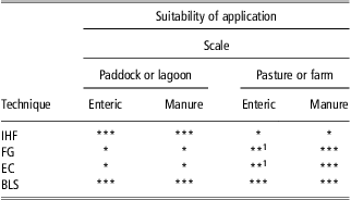
A few studies report the comparison of different micrometeorological techniques within a study. Laubach et al. (2008) reported a good fit of CH4 emissions from cattle in small paddocks when using the BLS, FG and IHF techniques (plus an enteric tracer technique) simultaneously, provided that a minimum separation between the paddock and sensor location exists when using the FG and IHF techniques. In their study, using 22 m separation, the BLS emissions were correlated with IHF (R 2 = 0.85) and FG (R 2 = 0.75); however, the BLS emissions were 20% higher than the two techniques. Laubach and Kelliher (Reference Laubach and Kelliher2005) reported the comparison of CH4 emissions for grazing dairy cows measured using the BLS technique against that of the FG and the IHF techniques. They concluded for their experimental design that the BLS (statistical errors of 15% to 20% when using point detection of concentration) and IHF (statistical errors of 10%) were preferred techniques over that of the FG technique. The FG technique was deemed to have higher uncertainty as a result of the need to use a footprint model when applying this technique to a finite area source; suitability is low (Table 1). Laubach and Kelliher (Reference Laubach and Kelliher2005) acknowledge that the BLS error may improve if line-averaged concentration measurements are used instead of point concentrations.
Summary of micrometeorological techniques regarding their application of methane emissions for animal agriculture
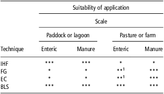
IHF = integrated horizontal flux; FG = flux gradient; EC = eddy covariance; BLS = backward Lagrangian stochastic.
1Requires evaluation of the footprint area and livestock density.
*Not recommended, **potential, ***most relevant.
Another way of determining accuracy of a micrometeorological technique is to release a tracer gas at a known flow rate and to use the technique to calculate a recovery rate. Ideally, the gas flow from a cylinder of gas is regulated by a mass flow controller during the release/recovery period, and the total gas released over the period is checked by weighing the cylinder before and after the release. The BLS technique has been tested by Ro et al. (Reference Ro, Johnson, Hunt and Flesch2011) who report a recovery of 98%, and McBain and Desjardins (Reference McBain and Desjardins2005) who recovered 106%. Gao et al. (Reference Gao, Desjardins and Flesch2009) found a recovery of 101% for the IHF technique and 103% for the BLS technique. Harper et al. (Reference Harper, Flesch, Powell, Coblentz, Jokela and Martin2009) reported (for ammonia) that the BLS technique estimated 100.1% recovery rates from known true release rates. McGinn et al. (2006) used BLS (WindTrax point source releases at a dairy) and reported recoveries of 86% and 100% for trace releases of CH4 and SF6, respectively. The low 86% recovery of CH4 was attributed to the presence of cattle (area source) confounding CH4 point source release. Previous release and recovery work by Flesch et al. (Reference Flesch, Wilson, Harper, Crenna and Sharpe2004), using an open-path laser, found that the BLS recovered 102% of the controlled release. Harper et al. (Reference Harper, Flesch, Weaver and Wilson2010) looked at a number of release/recovery BLS studies and concluded the BLS accuracy was 100 ± 10%.
A related accuracy challenge when comparing enteric CH4 emissions from different treatments (e.g., dietary) is the need to normalize the emissions by dividing by the DMI. This procedure removes the effect of the amount of intake (Grainger et al., Reference Grainger, Clarke, McGinn, Auldist, Beauchemin, Hannah, Waghorn, Clark and Eckard2007), allowing a focus on more relevant factors. Inaccuracy in measuring DMI, especially for grazing animals, contributes to inaccuracy of emission studies. For production systems where the feed is highly regulated, measuring DMI is more direct than that from grazing animals. Other indices reported is the CH4 emission per kg digestible DMI, per MJ (gross energy) of the feed or per production amount (kg milk or meat), where inaccuracies add to the overall error in the CH4 emission factor.
CH4 concentration detection and wind statistics
Fundamental to all micrometeorological techniques is the requirement for accurate and precise measurement of concentration, at a resolution high enough to detect differences between the background and the elevated source concentration associated with the source or between treatment concentrations. A number of detectors exist, such as those outlined by Neftel et al. (Reference Neftel, Fischer and Flechard2006) including three commonly used approaches, that is, laser and Fourier transform infrared (FTIR) spectroscopy, and infrared gas analysers.
Open-path CH4 lasers (e.g., Boreal Lasers Inc., model GasFinder, Edmonton, AB, Canada) have been used in the BLS technique for some time to detect the line concentration of CH4 (Flesch et al., 2009; Gao et al., Reference Gao, Desjardins and Flesch2009; McGinn and Beauchemin, 2012). Where the CH4 concentration associated with the source is close to the background concentration, the error in calculating the difference is large, and the emission value is uncertain.
Recently, the open-path laser and FTIR have been used in conjunction with a digitized stepping motor (scanner) to allow multi-path CH4 concentrations measurements using one laser or FTIR unit, thus avoiding the problem of between-sensor differences (e.g., drifting and offsets). The elimination of the between-sensor differences increases the resolution of the horizontal concentration gradient that can be measured (downwind–upwind concentration). This is especially significant when the source strength is weak, that is, in the case of low stocking rates (animals per ha) of grazing ruminants. The scanner when used with an open-path laser can also be programmed to optimize light-return levels, which can otherwise drift when the laser beam misaligns with its reflector that is more common over longer paths.
The recent development of the fast-response CH4 open-path sensor proved sensitive to the presence of grazing cattle (Baldocchi et al., Reference Baldocchi, Detto, Sonnentag, Verfaillie, Teh, Silver and Kelly2012) and was used to measure enteric CH4 emissions from grazing sheep (Dengel et al., Reference Dengel, Levy, Grace, Jones and Skiba2011) when supported by footprint analysis.
The EC and BLS techniques require information on atmospheric turbulence that is quantified using a three-dimensional sonic anemometer. Typically, this sensor is mounted (leveled) over the source area at a height of 2 to 3 m. The high-frequency outputs of the sensor are the vertical (w) and two horizontal (u and v) wind speeds, plus their cross products (uu, vv, ww, uv, uw, vw). These data are averaged over 10 to 30 min intervals generally, and a two-stage rotation (Kaimal and Finnigan, Reference Kaimal and Finnigan1994) is carried out to set the mean w and v to zero. The algorithms to extract the turbulence data (e.g., EddyPro software; LI-COR Biosciences; WindTrax) has become more user-friendly, allowing the non-micrometeorologist access to EC and BLS techniques.
Summary
Considerable expertise is needed to successfully apply micrometeorological techniques to measure CH4 emissions from livestock and livestock manure. This is especially the case where these techniques are deployed to measure small differences between treatments as part of a mitigation investigation.
The ease of application depends on many factors, including the scale of the emission. The IHF (MMD) technique is perhaps most straightforward, but still requires some assumptions regarding the time averaging of measurements. No assumptions are needed regarding the characteristics of the source distribution or strength, but a minimum separation distance between source and concentration detection is required. Practical limitations exist, such as the small paddock size that limits the measurement period of grazing ruminants (pending the stocking rate and forage available), and the number of concentration and wind speed measurements that are needed. The FG and the EC techniques are theoretically more demanding and are intended for large area and uniform CH4 sources. Neither of these techniques are recommended for measuring enteric CH4 from grazing cattle on pasture unless a footprint is known and the movement of the cattle is monitored (e.g., using camera or GPS). The BLS technique is a promising approach that has application for all scales (Table 1) including grazing ruminants that are confined in a paddock.
Recent developments in micrometeorological techniques have focused on better detection and greater understanding of the limitations and determining the accuracy of these techniques. For example, in the BLS technique when using WindTrax, more precise data filtering criteria has improved the quantity of useable emission data. In addition, advancements in the instrumentation (e.g., open-path lasers) used in micrometeorological techniques have improved the resolution of the CH4 concentration and increased the accuracy/precision of the techniques. The availability of a fast response detector for CH4 concentration now allows EC applications. Improvements in the field configuration, where one sensor (e.g., open-path laser) mounted on a scanner can replace the need for multiple sensors eliminate the between-sensor error.
Some micrometeorological techniques are best suited to evaluate herd scale (small paddocks of livestock) and manure storage facilities CH4 emissions, and offer the opportunity to investigate mitigation strategies. A greater challenge exists when using these techniques for large-scale (pastoral) grazing livestock where the source strength is weak. It is expected that further instrumentation developments in the measurement of concentration, and increased understanding of the constraints to estimating emissions, will continue to advance the application of micrometeorological techniques.
Acknowledgements
This paper was published as part of a supplement to animal, publication of which was supported by the Greenhouse Gases & Animal Agriculture Conference 2013. The papers included in this supplement were invited by the Guest Editors and have undergone the standard journal formal review process. They may be cited. The Guest Editors appointed to this supplement are R. J. Dewhurst, D. R. Chadwick, E. Charmley, N. M. Holden, D. A. Kenny, G. Lanigan, D. Moran, C. J. Newbold, P. O'Kiely, and T. Yan. The Guest Editors declare no conflict of interest.