3.1 Governing equations

In order to remove the singularity in expression (2.2) for the pressure, when $h(z,t)\rightarrow 0$, we define the interface radius $h(z,t)$ in terms of the function $a(z,t)$ where $a=h^{2}$. The governing equations (2.1) thus transform into

(3.1a)$$\begin{eqnarray}\displaystyle & \displaystyle \frac{\unicode[STIX]{x2202}a}{\unicode[STIX]{x2202}t}=-\frac{\unicode[STIX]{x2202}}{\unicode[STIX]{x2202}z}(au), & \displaystyle\end{eqnarray}$$

(3.1b)$$\begin{eqnarray}\displaystyle & \displaystyle \frac{\unicode[STIX]{x2202}u}{\unicode[STIX]{x2202}t}=-u\frac{\unicode[STIX]{x2202}u}{\unicode[STIX]{x2202}z}-\frac{\unicode[STIX]{x2202}p}{\unicode[STIX]{x2202}z}+3Oh_{in}\left(\frac{\unicode[STIX]{x2202}}{\unicode[STIX]{x2202}z}\left(a\frac{\unicode[STIX]{x2202}u}{\unicode[STIX]{x2202}z}\right)\frac{1}{a}\right)+Bo_{in}, & \displaystyle\end{eqnarray}$$

(3.1c)$$\begin{eqnarray}\displaystyle & \displaystyle p=\left(\frac{\displaystyle \left(2-\frac{\unicode[STIX]{x2202}^{2}a}{\unicode[STIX]{x2202}z^{2}}\right)a+\left(\frac{\unicode[STIX]{x2202}a}{\unicode[STIX]{x2202}z}\right)^{2}}{\displaystyle 2\left(\frac{1}{4}\left(\frac{\unicode[STIX]{x2202}a}{\unicode[STIX]{x2202}z}\right)^{2}+a\right)^{3/2}}\right). & \displaystyle\end{eqnarray}$$

$(a_{b}=h_{b}^{2})$

(3.2)$$\begin{eqnarray}u_{f}(0,t)=\text{Re}(\unicode[STIX]{x1D716}\text{e}^{\text{i}\unicode[STIX]{x1D714}t}),\end{eqnarray}$$

where $\unicode[STIX]{x1D716}$ represents the amplitude of the forcing and $\unicode[STIX]{x1D714}$ represents the angular forcing frequency. In the presence of the forcing, the boundary conditions at the inlet are modified to $a(0,t)=1$ and $u(0,t)=\sqrt{We_{in}}+u_{f}$. No boundary conditions are defined at the other extremity of the domain close to the tip. Nonetheless, a special treatment is applied for the tip, as explained in the next section.

3.2 Numerical scheme

The governing equations (3.1) are first discretised in space, after which the resulting ordinary differential equations (ODEs) are integrated in time. Diffusion terms are evaluated using second-order finite differences, with a central scheme for intermediate nodes and a forward or backward scheme for boundary nodes. Advection terms are obtained using a weighted upwind scheme inspired by Spalding’s (Reference Spalding1972) hybrid difference scheme. Unlike the latter, which approximates the convective derivative using a combination of central and upwind schemes, we evaluate the derivative based on a combination of forward and backward finite differences. An advection term $\text{d}A/\text{d}z$ is evaluated at node $i$ as

(3.3)$$\begin{eqnarray}\left(\frac{\text{d}A}{\text{d}z}\right)_{i}=\unicode[STIX]{x1D6FD}\left(\frac{\text{d}A}{\text{d}z}\right)_{i,b}+(1-\unicode[STIX]{x1D6FD})\left(\frac{\text{d}A}{\text{d}z}\right)_{i,f},\end{eqnarray}$$

where indices $b$ and $f$ refer to the backward and forward finite difference schemes, and $\unicode[STIX]{x1D6FD}$ is a weight coefficient that depends on the local value of velocity $u$ at node $i$ together with a parameter $\unicode[STIX]{x1D6FC}$:

(3.4)$$\begin{eqnarray}\unicode[STIX]{x1D6FD}=\frac{\tanh (\unicode[STIX]{x1D6FC}u_{i})+1}{2}.\end{eqnarray}$$

For the range of feed velocities considered in this study, numerical stability was always ensured by using a 10-point stencil. Thus, the backward difference term relies on a stencil that spans nodes $i-5$ to $i+4$, and the forward difference term employs nodes $i-4$ to $i+5$. For large enough downstream or upstream velocities, $\unicode[STIX]{x1D6FD}$ will tend to $1$ or $0$, respectively; hence (3.3) reduces to a regular upwind difference scheme. For smaller velocity magnitudes in between, (3.3) produces a weighted combination of backward and forward differences. In our simulations, we choose $\unicode[STIX]{x1D6FC}=50$ so that the transition between the backward and forward difference schemes mostly occurs when $|u|<0.05$. Finally, advection terms at nodes close to the boundary are evaluated based on the values of the closest nine adjoining nodes.

After obtaining all spatial derivatives, the resulting ODEs are integrated using the MATLAB solver ode23tb, which implements a trapezoidal rule and a backward differentiation formula known as TR-BDF2 (Bank et al. Reference Bank, Coughran, Fichtner, Grosse, Rose and Smith1985), and uses a variable time step to reduce the overall simulation time.

The numerical domain $L$ is taken sufficiently large to capture the breakup of the jet. The jet interface is initialised by the solution of (2.5) obtained numerically with the MATLAB bvp4c solver. The corresponding velocity at each axial location is then obtained by equating the interface radius with the constant inlet flow rate $Q$. The validation of the numerically obtained base-state solution for the jet interface is presented in § A.1. It should be noted that the jet is initialised only for a segment of the domain $L$ with the steady-state equation. For the remaining segment of the domain, both the jet radius and its velocity are initialised to zero. Defining the initial conditions with the base-state solution only for a part of the domain $L$ helps to reduce the computational cost without any loss in the accuracy of the results obtained. The axial span of the base-state solution does not affect the quasi-steady jet characteristics, which are the focal point of our numerical analysis. A validation for the same is presented in § A.2.

At every time step, the solution is evaluated for three conditions:

1. (i) Pinch-off (breakup). This is defined as when the value of $a$ passes below a threshold value of $10^{-5}$. The corresponding time $t_{po}$ is saved and the position of the jet tip is updated as $N_{tip}=N_{po}$, where $N_{po}$ is the pinch-off location. The solution for $a$ and $u$ beyond $N_{tip}$ is set to zero. For subsequent time steps, $N_{tip}$ has two possibilities – it can either advance or recede, which requires the following two conditions.

2. (ii) Advancing jet. The values of $a$ at nodes $N_{tip}-1$ and $N_{tip}$ are extrapolated to find $a$ at $N_{tip}+1$. If the extrapolated value is larger than a predefined value of $5\times 10^{-3}$, the parameter $N_{tip}$ is incremented by 1, and $a$ and $u$ at the new $N_{tip}$ are assigned values extrapolated from its previous two neighbours.

3. (iii) Receding jet. If the value of $f$ at $N_{tip}$ falls below a predefined value of $10^{-3}$, $a$ and $u$ at $N_{tip}$ are set to zero and the parameter $N_{tip}$ is reduced by 1.

These three conditions enable the numerical integration of the governing equations in a way that captures accurately the breakup of the jet and the motion of the tip. A validation of the numerical scheme is presented in § A.3.

3.3 Nonlinear simulation results

Using the numerical scheme presented in the previous section, nonlinear simulations were performed for a jet governed by (3.1) for fixed inlet characteristics: $Oh_{in}=0.3$, $We_{in}=1.75$ and $Bo_{in}=0.1$. The jet inlet velocity is subjected to time-harmonic forcing of the form given by (3.2) with a fixed amplitude $\unicode[STIX]{x1D716}$ and for forcing frequency$\unicode[STIX]{x1D714}=[0.4-3.2]$.

The simulations were run for a sufficiently long time to enter a permanent regime wherein the jet breaks up at regular intervals of time and at fixed axial location. In the quasi-steady regime, the breakup period $\unicode[STIX]{x0394}T_{po}$ is defined as the time difference between two consecutive breakups or pinch-offs and the breakup length $l_{c}$ as the stable length of the jet between the nozzle and the pinch-off location. We use $l_{c}$ as the quantifier to determine the stability of the jet to external forcing such that the most amplified disturbance caused by the optimal frequency $\unicode[STIX]{x1D714}_{opt}$ will compel the jet to have the shortest possible breakup length.

Figure 1.

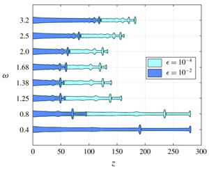
The jet intact shape along the axial direction $z$ for a gravity jet defined by $Oh_{in}=0.3$, $Bo_{in}=0.1$ and $We_{in}=1.75$ and perturbed by different inlet forcing frequencies $\unicode[STIX]{x1D714}$ and forcing amplitudes $\unicode[STIX]{x1D716}=10^{-2}$ and $\unicode[STIX]{x1D716}=10^{-4}$. For clarity, only the shape corresponding to the shortest breakup length for every frequency is plotted. The forcing frequencies are in steps of $\unicode[STIX]{x1D6FF}=0.4$ except for certain intermediate ranges highlighted by the axis break symbol. The jets of two different colours represent the shape at the same forcing frequency but different forcing amplitudes $\unicode[STIX]{x1D716}$. We see that for $\unicode[STIX]{x1D716}=10^{-2}$ the breakup length is the minimum for $\unicode[STIX]{x1D714}=1.38$ and for $\unicode[STIX]{x1D716}=10^{-4}$ it is minimum for $\unicode[STIX]{x1D714}=1.68$. The box in red shows the zoomed image of the jet close to a breakup, highlighting the existence of a satellite and a main drop. The zoomed image has radial $h$ and axial $z$ dimensions drawn to the same scale, each representing a dimensionless size of 6. The red bar in both the plots represents a dimensionless radial length scale of 2, which is also the size of the dimensionless nozzle diameter.

We begin our analysis for fixed amplitudes $\unicode[STIX]{x1D716}=10^{-2}$ and $\unicode[STIX]{x1D716}=10^{-4}$. The response of the jet due to different forcing frequency $\unicode[STIX]{x1D714}$ in the permanent regime for the two above-mentioned amplitudes can be seen in figure 1. Jets enforced by the same disturbance amplitude at the inlet are represented by the same colour. For visual clarity we plot the response only for certain frequencies and for the jet shape pertaining to the shortest breakup length. First, figure 1 clearly shows the existence of a main drop and a satellite drop for all the frequencies. Second, for $\unicode[STIX]{x1D716}=10^{-2}$ we conclude that the optimal forcing frequency is $\unicode[STIX]{x1D714}_{opt}=1.38$ because it manifests the jet to have the shortest $l_{c}$. Third, and most strikingly, we notice that for a lower forcing amplitude of $\unicode[STIX]{x1D716}=10^{-4}$, the optimal forcing increases to $\unicode[STIX]{x1D714}_{opt}=1.68$. We would like to highlight here that a similar inverse relation between the forcing amplitude and the optimal forcing frequency for gravitationally stretched jets can also be observed through the linear response analysis results presented in Consoli-Lizzi et al. (Reference Consoli-Lizzi, Coenen and Sevilla2014) and Consoli-Lizzi (Reference Consoli-Lizzi2016). Finally, at all forcing frequencies, the breakup length for the jet with $\unicode[STIX]{x1D716}=10^{-4}$ is always larger than for $\unicode[STIX]{x1D716}=10^{-2}$.

To investigate further the breakup characteristics for the amplitudes $\unicode[STIX]{x1D716}=10^{-2}$ and $\unicode[STIX]{x1D716}=10^{-4}$ due to $\unicode[STIX]{x1D714}_{opt}$, we plot the interface evolution in the permanent regime as shown in figures 2(a) and 2(c), where regular-sized main drop formation is followed by the release of a satellite drop. For both the amplitudes, we see a distinct difference between the main and satellite drop radii.

Figure 2.

Breakup characteristics for a gravity jet defined by $Oh_{in}=0.3$, $Bo_{in}=0.1$ and $We_{in}=1.75$ and perturbed with $\unicode[STIX]{x1D714}_{opt}$. Panels (a,b) correspond to a forcing with $\unicode[STIX]{x1D716}=10^{-2}$ and $\unicode[STIX]{x1D714}_{opt}=1.38$; and panels (c,d) refer to a forcing with $\unicode[STIX]{x1D716}=10^{-4}$ and $\unicode[STIX]{x1D714}_{opt}=1.68$. In panels (a,c) is elaborated the interface profile at the time of breakup with the existence of a satellite drop after the main drop is released. The main and satellite drop radii for both the cases have been highlighted. The axial and radial dimensions of (a,c) represent the same length scale. In panels (b,d) is represented the breakup period $\unicode[STIX]{x0394}T_{po}$. The black triangles refer to $\unicode[STIX]{x0394}T_{po}$ between consecutive drops and the blue circles represent that between two consecutive main (or satellite) drops. The breakup frequency $\unicode[STIX]{x1D714}_{po}$ is equal to 1.38 and 1.68 in (b,d) respectively.

The breakup period $\unicode[STIX]{x0394}T_{po}$ resulting from the forcing imposed in figures 2(a) and 2(c) are plotted in figures 2(b) and 2(d), respectively, where the black triangles represent the $\unicode[STIX]{x0394}T_{po}$ obtained for two consecutive pinch-offs whereas the blue circles denote $\unicode[STIX]{x0394}T_{po}$ obtained for two consecutive main (or satellite) drop pinch-offs. The latter is observed to be the same for the main and satellite drop formation (as shown in blue circles). However, the time of formation of a satellite drop does not lie exactly midway between the time of formation of the main drops and vice versa. This results in obtaining two oscillating breakup periods (as shown by the black triangles). We further observe that the frequency of breakup ($\unicode[STIX]{x1D714}_{po}=2\unicode[STIX]{x03C0}/\unicode[STIX]{x0394}T_{po}$) obtained using the breakup period for consecutive main (or satellite) drops responds to the externally applied forcing at the jet inlet. For forcing amplitudes $\unicode[STIX]{x1D716}=10^{-2}$ and $10^{-4}$, $\unicode[STIX]{x1D714}_{po}=1.38$ and $1.68$, respectively.

Finally, for the constant flow rate of the jet, the breakup period related to the consecutive pinch-offs is used to obtain the drop radius for the satellite and main drops. Note here that the definition of the main and satellite drop radii coincide with the classical definition of volume-equivalent radii. We notice that, at the optimal forcing frequency, the main drop radius $R_{m}$ decreases from 1.62 to 1.48 dimensionless units as $\unicode[STIX]{x1D716}$ reduces from $10^{-2}$ to $10^{-4}$. On the contrary, the satellite drop radius $R_{s}$ increases from 0.78 to 1.08 dimensionless units for $\unicode[STIX]{x1D716}=10^{-2}$ and $\unicode[STIX]{x1D716}=10^{-4}$, respectively. The longer intact jet length obtained for lower forcing amplitude $\unicode[STIX]{x1D716}=10^{-4}$ results in a larger downstream velocity close to the tip due to the presence of gravity. Eventually, it results in the formation of highly stretched satellite drops in comparison to the ones obtained for lower amplitude of $\unicode[STIX]{x1D716}=10^{-2}$ as seen in figure 2(a,c).

Figure 3.

The breakup length $l_{c}$ as a function of forcing frequency $\unicode[STIX]{x1D714}$ for a gravity jet defined by $Oh_{in}=0.3$, $Bo_{in}=0.1$ and $We_{in}=1.75$. Each curve is indicative of a fixed forcing amplitude $\unicode[STIX]{x1D716}$. For a fixed $\unicode[STIX]{x1D716}$, the optimal forcing frequency related to the shortest $l_{c}$ is represented by a red cross. We observe that the optimal frequency increases as $\unicode[STIX]{x1D716}$ decreases and does not appear to saturate even for lower amplitudes of $10^{-8}$. The black circles represent the data from numerical simulations.

We now return to the most salient feature observed in figure 1, where the optimal forcing frequency $\unicode[STIX]{x1D714}_{opt}$ increased with a decrease in forcing amplitude. To explore if this effect existed for smaller amplitudes, we simulated the same system for different forcing amplitudes $\unicode[STIX]{x1D716}=[10^{-2}{-}10^{-8}]$, and plotted the breakup length $l_{c}$ as a function of the forcing frequency $\unicode[STIX]{x1D714}$ as shown in figure 3, where the optimal forcing frequency for a fixed $\unicode[STIX]{x1D716}$ is marked with a red cross. The results show an increase in $l_{c}$ and $\unicode[STIX]{x1D714}_{opt}$ as $\unicode[STIX]{x1D716}$ decreases, which is in qualitative agreement with the linear response analysis results presented in Consoli-Lizzi (Reference Consoli-Lizzi2016). The increase in breakup length is obvious due to the decreasing destabilising strength of the forcing amplitude. The increase in optimal forcing frequency, however, is the most interesting observation drawn from the numerical results, since it is expected to saturate for small enough forcing amplitudes. The increase in $\unicode[STIX]{x1D714}_{opt}$ as $\unicode[STIX]{x1D716}$ decreases from $10^{-2}$ to $10^{-8}$ is a consequence of the stretched base state due to gravity, which results in the downstream stretching of the perturbation wavelength initiated at the nozzle. As the forcing amplitude decreases, the stable jet length $l_{c}$ increases and so does the stretching close to the jet tip. Thus to compensate for the larger stretching, the breakup potential of the forcing is sustained by increasing the forcing frequency.

To conclude, the numerical simulations confirm the dependence of $\unicode[STIX]{x1D714}_{opt}$ on the forcing amplitude, a factor generally neglected for linear stability analysis as long as $\unicode[STIX]{x1D716}\ll 1$. The trend also constitutes a major difference from a jet with no gravity effect ($Bo_{in}=0$), where $\unicode[STIX]{x1D714}_{opt}$ is independent of $\unicode[STIX]{x1D716}$ (see figure 20 in § A.4). Finally, we confirm that the preferred-mode analysis carried out for the jet is solely due to the effect of external forcing. For the given parameter range, the jet tip did not induce any self-sustained breakups.

4.1 Local stability analysis for jets in the absence of gravity

We derive the dispersion relation for the coupled equations (2.1), governing the growth of small perturbations about the base state. Considering the normal-mode expansion, the flow variables $h(z,t)$ and $u(z,t)$ are decomposed as

(4.1a)$$\begin{eqnarray}\displaystyle & \displaystyle h(z,t)=h_{b}+\unicode[STIX]{x1D716}{\hat{h}}\text{e}^{\text{i}(kz-\unicode[STIX]{x1D714}t)}, & \displaystyle\end{eqnarray}$$

(4.1b)$$\begin{eqnarray}\displaystyle & \displaystyle u(z,t)=u_{b}+\unicode[STIX]{x1D716}\hat{u} \text{e}^{\text{i}(kz-\unicode[STIX]{x1D714}t)}, & \displaystyle\end{eqnarray}$$

$\unicode[STIX]{x1D716}\ll 1$

${\hat{h}}$

$\hat{u}$

$k$

$\unicode[STIX]{x1D714}$

$a(z,t)$

(4.2)$$\begin{eqnarray}a(z,t)=a_{b}+\unicode[STIX]{x1D716}\hat{a}\text{e}^{\text{i}(kz-\unicode[STIX]{x1D714}t)},\end{eqnarray}$$

where $a_{b}=h_{b}^{2}$ and $\hat{a}=2h_{b}{\hat{h}}$. Inserting the above expansion into (2.1), linearising about $(h_{b},u_{b})$ and replacing $h^{2}\rightarrow a$ will lead to a linearised system of equations, which can be formulated as an eigenvalue problem with the eigenmodes represented by $\hat{\boldsymbol{q}}=[\hat{a},\hat{u} ]$.

In the absence of gravity, $\hat{\boldsymbol{q}}$ represents a constant independent of $z$, $u_{b}=\sqrt{We}$ and $h_{b}=1$. Combining both the linearised continuity and momentum equations leads to the dispersion relation

(4.3)$$\begin{eqnarray}\unicode[STIX]{x1D714}=\sqrt{We}\,k-\frac{3\text{i}Ohk^{2}}{2}\pm \text{i}\sqrt{\frac{(k^{2}-k^{4})}{2}+\frac{9Oh^{2}k^{4}}{4}},\end{eqnarray}$$

where $Oh$ is constant throughout the domain. The dispersion relation is used to perform a spatio-temporal stability analysis, which includes the effect of advection speed of the jet on its stability properties. In this framework, we define the impulse response of a system to a localised perturbation that generates a wavepacket growing in space and time. In the laboratory framework, the spatio-temporal behaviour of the wavepacket can be described in terms of the complex absolute wavenumber $k_{0}$ and the corresponding complex absolute frequency $\unicode[STIX]{x1D714}_{0}=\unicode[STIX]{x1D714}(k_{0})$ whose imaginary part $\unicode[STIX]{x1D714}_{0,i}$ will determine the temporal evolution of the wavepacket. For $\unicode[STIX]{x1D714}_{0,i}>0$ the system is absolutely unstable since the disturbance grows fast enough to invade the entire domain in the laboratory frame; and for $\unicode[STIX]{x1D714}_{0,i}<0$ the system is convectively unstable as the localised perturbations are allowed to convect downstream before they grow in the laboratory frame. The complex pair ($k_{0},\unicode[STIX]{x1D714}_{0}$) is defined using the saddle point condition or the Briggs–Bers zero-group-velocity criterion, together with the dispersion relation

(4.4)$$\begin{eqnarray}\frac{\text{d}\unicode[STIX]{x1D6E5}(\unicode[STIX]{x1D714}_{0},k_{0})}{\text{d}k}=0,\quad \unicode[STIX]{x1D6E5}(\unicode[STIX]{x1D714}_{0},k_{0})=0,\end{eqnarray}$$

where $\unicode[STIX]{x1D6E5}$ represents the dispersion relation (4.3) and

(4.5)$$\begin{eqnarray}\frac{\unicode[STIX]{x2202}\unicode[STIX]{x1D6E5}}{\unicode[STIX]{x2202}k}=\sqrt{We}-3\text{i}Ohk\pm \text{i}\frac{1-2k^{2}+(3Ohk)^{2}}{\sqrt{2(1-k^{2})+(3Ohk)^{2}}}.\end{eqnarray}$$

Equation (4.4) identifies the critical dimensionless speed $We_{crit}$, for a fixed $Oh$, which signifies the transition of the jet from an absolutely unstable to a convectively unstable system as shown in figure 4 with the full and dashed lines. The two curves are obtained for a system initialised either using a low or a high $Oh$, respectively. For the intermediate values of $Oh$, we obtain two saddle points, thus giving two distinct values of the critical curve.

Figure 4.

The absolute–convective transition (represented by full and dashed lines) for viscous jets ($Bo_{in}=0$). The local variation in $Oh_{z}$ and $We_{z}$ for three jets with different $We_{in}$ (constant $Oh_{in}=0.3$, $Bo_{in}=0.1$, $L=50$) are plotted with different markers, where the red cross for each represents the inlet condition at $z=0$. The distance between consecutive markers for the same jet represents an axial gap of 10 units.

4.2 Local stability analysis for jets in the presence of gravity

Extending the formalism for parallel jets to spatially varying jets, we derive the dispersion relation for the coupled equations (2.1), governing the growth of small perturbations about the base state. The linearised system of equations obtained around the spatially varying base flow can be formulated as an eigenvalue problem with the eigenmodes represented by $\hat{\boldsymbol{q}}(\boldsymbol{z})=[\hat{a}(z),\hat{u} (z)]$ as functions of $z$. Next we express the local stability of a gravity jet by introducing the terms $Oh_{z}$ and $We_{z}$, which are the local dimensionless numbers at an axial distance of $z$ from the nozzle. They are expressed as

(4.6a)$$\begin{eqnarray}\displaystyle & \displaystyle Oh_{z}=Oh_{in}\sqrt{\frac{h_{b}(0)}{h_{b}(z)}}, & \displaystyle\end{eqnarray}$$

(4.6b)$$\begin{eqnarray}\displaystyle & \displaystyle We_{z}=h_{b}(z)u_{b}^{2}(z). & \displaystyle\end{eqnarray}$$

$Oh_{z}$

$We_{z}$

$L$

$Oh_{z}$

$We_{z}$

$L=50$

$Oh_{in}=0.3$

$Bo_{in}=0.1$

$We_{in}=[1.75,0.25,0.002]$

$We_{in}=1.75$

For $We_{in}=1.75$ and $0.002$, the entire jet exists in the convective and absolute region, respectively. For intermediate $We_{in}=0.25$, there exists a small pocket of absolute instability close to the nozzle, after which the local parameters modify along the downstream direction, resulting in the transfer of the jet into a convectively unstable regime.

The parameter $Bo_{in}$ indirectly affects the instability of the jet through the base-state solution. Since $Bo_{in}$ is constant, its relative strength for the stretching of the jet interface depends on the corresponding value of $We_{in}$, with the effect being more pronounced for lower values of $We_{in}$ as shown in figure 5.

Figure 5.

The stretching (or necking) close to the nozzle of the base flow due to the presence of gravity for a jet with $Oh_{in}=0.3$, $Bo_{in}=0.1$ and three different $We_{in}$. Clearly, the effect of gravity is prominent for the jet with the smallest $We_{in}$.

Next, for the spatially varying base flow, we perform the stability analysis in a local framework wherein the system is considered parallel at each axial location. The local dispersion relation, which now includes the local spatially varying base flow properties, is given by

(4.7)$$\begin{eqnarray}\unicode[STIX]{x1D714}^{2}-2u_{b}(z)\unicode[STIX]{x1D714}k+\left(\frac{1}{2\sqrt{a_{b}(z)}}+u_{b}(z)^{2}+3\text{i}Oh_{z}\unicode[STIX]{x1D714}\right)k^{2}-3\text{i}Oh_{z}u_{b}(z)k^{3}-\frac{\sqrt{a_{b}(z)}}{2}k^{4}=0.\end{eqnarray}$$

For the convectively unstable jet ($We_{in}=1.75$), the solution of the dispersion relation (4.7) for a given range of complex $\unicode[STIX]{x1D714}$ (with $\unicode[STIX]{x1D714}_{i}>0$) results in obtaining four spatial branches, which are expressed as the roots of the fourth-order polynomial (4.7). The solution consists of upstream-propagating (denoted $k^{-}$) and downstream-propagating (denoted $k^{+}$) branches. To identify these branches, we successively add an artificial $\unicode[STIX]{x1D714}_{i}$ so as to separate the branches into the upper $k_{i}>0$ and lower $k_{i}<0$ planes (Huerre & Rossi Reference Huerre and Rossi1998; Gallaire & Brun Reference Gallaire and Brun2017). For a downstream-propagating $k^{+}$ branch damped in space, the associated $k_{i}>0$. Based on this analysis, we obtain two downstream- and two upstream-propagating waves for the dispersion relation (4.7). The $k$ branches for the localised dimensionless numbers at the nozzle inlet ($z=0$) and domain end ($z=50$) are shown in figure 6(a) and 6(b), respectively, with the two $k^{+}$ branches denoted by the black and green colours and the two $k^{-}$ waves by the red and blue colours. The presence of two $k^{+}$ and $k^{-}$ waves is not specific to the present jet characteristics but rather exists for all the tested cases in the range of $Oh_{in}=[0.1,~10]$, $We_{in}=[0.8,~10]$ and $Bo_{in}=[0,~1]$ for $L=50$.

Figure 6.

The four $k$ branches shown in four different colours, obtained as a solution of the dispersion relation for complex $\unicode[STIX]{x1D714}$ and for increasing values of $\unicode[STIX]{x1D714}_{i}$ for a jet defined by $Oh_{in}=0.3$, $Bo_{in}=0.1$ and $We_{in}=1.75$ at (a) the nozzle outlet $z=0$ and (b) the jet exit $z=L=50$. The arrows represent the direction of movement of the waves for increasing values of $\unicode[STIX]{x1D714}_{i}$.

4.3 Spatial stability analysis

Since the base flow with $We_{in}=1.75$ exists in the convectively unstable regime (see figure 4), we then proceed to analyse the base flow using the spatial stability framework, wherein the spatial growth rate for the imposed real frequency determines the flow stability.

Figure 7.

(a) Growth rate $-k_{i}$ for a jet defined by $Oh_{in}=0.3$, $Bo_{in}=0.1$ and $We_{in}=1.75$, plotted as a function of the frequency for the four $k$ branches at the nozzle exit with the dominant $k$ branch represented in black. (b) The growth rate corresponding to the dominant $k$ branch at different axial locations. The inset shows the evolution of the locus of the real and imaginary parts of $\hat{u} _{r}$ and $\hat{u} _{i}$ at the optimal frequency as $z$ increases. (c) The growth rate $-k_{i}$ of the dominant $k$ branch as a function of $z$ for various $\unicode[STIX]{x1D714}$. (d) The $k_{r}$ related to the optimal growth rate in (b) as a function of real frequency. The coloured markers (●) in (b) and (d) correspond to the same forcing frequency and the axial location.

Given the polynomial nature of the dispersion relation, there are four spatial waves. We have verified that two of them are $k^{+}$, downstream-propagating, waves while the remaining two are $k^{-}$, upstream-propagating, waves (see figure 6). For a more detailed account on the nature of spatial waves in capillary jets, depending on the flow model, the reader is referred to Guerrero, González & García (Reference Guerrero, González and García2016).

Among the four $k$ waves, only one of the $k^{+}$ waves is seen to be amplified. To obtain this dominant $k$ wave, we plot the spatial growth rate $-k_{i}$ as a function of the real forcing frequency $\unicode[STIX]{x1D714}$ at the nozzle inlet. As shown in figure 7(a), among the four $k$ branches, only the branch denoted in black has a growth rate that is positive in its propagation direction. We chose the $k$ wave corresponding to this amplified $k^{+}$ branch as the dominant wavenumber for all frequencies. The relevant $k(z)$ branches are then obtained for different $z$ along the jet as shown in figure 7(b,d) by imposing the spatially dependent base flow and $Oh_{z}$ in (4.7). Figure 7(b) shows that the most amplified frequency shifts to higher values as one travels away from the nozzle. The associated eigenmode $\hat{\boldsymbol{q}}(z)$ also changes as one progresses downstream. Imposing $\Vert \hat{\boldsymbol{q}}\Vert =1$ at every axial location as the normalisation condition, together with $\hat{a}_{i}=0$ to set the phase, we see in figure 7(c) the evolution of the locus of the real and imaginary parts of the remaining degrees of freedom $\hat{u} _{r}$ and $\hat{u} _{i}$ as $z$ increases (remember that $\hat{u} _{r}^{2}+\hat{u} _{i}^{2}+\hat{a}_{r}^{2}=1$). While this locus is difficult to interpret from a physical point of view, it highlights the change of the eigenmode along the jet axis in such non-parallel gravity-driven jets.

The knowledge of the relevant $k^{+}$ wave obtained for a given $\unicode[STIX]{x1D714}$ allows us to evaluate the leading-order response due to different forcing frequencies imposed on the base flow, conveniently expressed as

(4.8)$$\begin{eqnarray}\boldsymbol{q}^{\prime }(z,t)=\hat{\boldsymbol{q}}(\unicode[STIX]{x1D714},z)\exp \!\left[\text{i}\left(\int _{0}^{z}k(\unicode[STIX]{x1D714},z^{\prime })\,\text{d}z^{\prime }-\unicode[STIX]{x1D714}t\right)\right].\end{eqnarray}$$

The overall response norm defined in a domain size $L$ is then given as

(4.9)$$\begin{eqnarray}G_{s}(\unicode[STIX]{x1D714},L)=\left\Vert \int _{0}^{L}\hat{\boldsymbol{q}}(\unicode[STIX]{x1D714},z)\exp \!\left[\text{i}\left(\int _{0}^{z}k(\unicode[STIX]{x1D714},z^{\prime })\,\text{d}z^{\prime }-\unicode[STIX]{x1D714}t\right)\right]\right\Vert .\end{eqnarray}$$

This allows us to determine the optimal forcing frequency $\unicode[STIX]{x1D714}_{opt}$ that results in the maximal gain

(4.10)$$\begin{eqnarray}G_{s,max}(L)=\underset{\unicode[STIX]{x1D714}}{\max }\;[G_{s}(\unicode[STIX]{x1D714},L)],\end{eqnarray}$$

attained at a frequency $\unicode[STIX]{x1D714}_{opt}$. Figure 8 (in dotted lines) shows the spatial gain as a function of forcing frequency for two arbitrary domain sizes $L=50$ and $60$. We notice that $\unicode[STIX]{x1D714}_{opt}$ shifts from 1.16 to 1.21 as we increase the domain size.

Figure 8.

Comparison of the total gain $G$ at different frequencies $\unicode[STIX]{x1D714}$ from the resolvent analysis and the spatial analysis for domain sizes (a) $L=50$ and (b) $L=60$ and for the jet defined by $Oh_{in}=0.3$, $Bo_{in}=0.1$ and $We_{in}=1.75$. The resolvent gain is computed by using the transfer function and the direct mode obtained from the spatial analysis. All the theories predict a shift in $\unicode[STIX]{x1D714}_{opt}$ as $L$ is increased.

4.4 Weakly non-parallel stability analysis (WKBJ)

In order to further incorporate the non-parallelism of the base flow, we extend our spatial analysis by including the WKBJ formalism introduced by Gaster et al. (Reference Gaster, Kit and Wygnanski1985) and Huerre & Rossi (Reference Huerre and Rossi1998) for a spatial mixing layer and applied by Viola et al. (Reference Viola, Arratia and Gallaire2016) for swirling flows.

In this framework, we introduce a slow streamwise scale $Z$, which relates to the fast scale $z$ as $Z=\unicode[STIX]{x1D702}z$, where $\unicode[STIX]{x1D702}\ll 1$ is a measure of the weak non-parallelism. The new base flow depends only on $Z$ and the global response to inlet forcing takes the modulated wave form

(4.11)$$\begin{eqnarray}\boldsymbol{q}^{\prime }(Z,t)\sim A(Z)\hat{\boldsymbol{q}}(Z,0)\exp \!\left[\text{i}\left(\frac{1}{\unicode[STIX]{x1D702}}\int _{0}^{Z}k(\unicode[STIX]{x1D714},Z^{\prime })\,\text{d}Z^{\prime }-\unicode[STIX]{x1D714}t\right)\right],\end{eqnarray}$$

where $\hat{\boldsymbol{q}}(\unicode[STIX]{x1D714},Z)$ is the local eigenmode and $k(\unicode[STIX]{x1D714},Z)$ the local wavenumber at section $Z$ and a fixed forcing frequency $\unicode[STIX]{x1D714}$. The amplitude function $A(Z)$ acts as an envelope, smoothly connecting the progressive slices of the parallel spatial analysis. At each axial location, we impose $\hat{\boldsymbol{q}}^{\text{H}}\boldsymbol{\cdot }\hat{\boldsymbol{q}}=1$, where $(\cdot )^{\text{H}}$ is the transconjugate. As described in § A.6, imposing an asymptotic expansion and a compatibility condition, the local stability analysis is retrieved at zeroth order in $\unicode[STIX]{x1D702}$, while at first order in $\unicode[STIX]{x1D702}$ the following amplitude equation is obtained:

(4.12)$$\begin{eqnarray}M(Z)\frac{\text{d}A(Z)}{\text{d}Z}+N(Z)A(Z)=0,\end{eqnarray}$$

whose solution is given as

(4.13)$$\begin{eqnarray}A(Z)=A_{0}\exp \!\left(-\int _{0}^{Z}\frac{N(Z^{\prime })}{M(Z^{\prime })}\,\text{d}Z^{\prime }\right).\end{eqnarray}$$

The functions $M(Z)$ and $N(Z)$ are defined in § A.6. The amplitude at the inlet is set as $A(0)=1$, which simplifies the forcing expression at the inlet to $\boldsymbol{q}^{\prime }(0,t)=\hat{\boldsymbol{q}}(0)\exp (\text{i}\unicode[STIX]{x1D714}t)$. Finally, we express the total spatial gain at first order as

(4.14)$$\begin{eqnarray}G_{Amp}^{2}(\unicode[STIX]{x1D714},L)=\frac{\displaystyle \int _{0}^{z}A^{\text{H}}(z^{\prime })A(z^{\prime })(\hat{\boldsymbol{q}}^{\text{H}}(z^{\prime })\boldsymbol{\cdot }\hat{\boldsymbol{q}}(z^{\prime }))\left[\exp \left(\int _{0}^{z^{\prime }}-2k_{i}(z^{\prime \prime })\,\text{d}z^{\prime \prime }\right)\right]\,\text{d}z^{\prime }}{\hat{\boldsymbol{q}}^{\text{H}}(0)\boldsymbol{\cdot }\hat{\boldsymbol{q}}(0)}.\end{eqnarray}$$

The global gain of the response due to the forcing frequency, for fixed domain sizes, is reported in figure 8, where $\unicode[STIX]{x1D714}_{opt}=1.24$ and $1.30$ for $L=50$ and $60$, respectively. The WKBJ approximation greatly modifies the gain when compared to the zeroth-order analysis and shifts the optimal forcing frequency predicted from the spatial analysis, which excludes the amplitude equation. However, to truly assess the validity of the amplitude equation, one needs to analyse the base flow in the global framework using the resolvent analysis, which will be the focus of our discussion in the next section.

5.1 Global stability

Since the base flow is spatially varying, the perturbations imposed on it are no longer sought in the form of Fourier modes but are expanded in the form

(5.1a)$$\begin{eqnarray}\displaystyle & \displaystyle h(z,t)=h_{b}(z)+\unicode[STIX]{x1D716}\tilde{h}(z)\text{e}^{\unicode[STIX]{x1D706}t}, & \displaystyle\end{eqnarray}$$

(5.1b)$$\begin{eqnarray}\displaystyle & \displaystyle u(z,t)=u_{b}(z)+\unicode[STIX]{x1D716}\tilde{u} (z)\text{e}^{\unicode[STIX]{x1D706}t}, & \displaystyle\end{eqnarray}$$

$\unicode[STIX]{x1D716}\ll 1$

$\tilde{h}(z)$

$\tilde{u} (z)$

$\unicode[STIX]{x1D706}$

$(h_{b},u_{b})$

(5.2)$$\begin{eqnarray}\unicode[STIX]{x1D706}\unicode[STIX]{x1D644}\left[\begin{array}{@{}c@{}}\tilde{h}\\ \tilde{u} \end{array}\right]=\unicode[STIX]{x1D648}\left[\begin{array}{@{}c@{}}\tilde{h}\\ \tilde{u} \end{array}\right],\end{eqnarray}$$

with boundary conditions $\tilde{h}(0,t)=0$ and $\tilde{u} (0,t)=0$. We do not impose any boundary conditions at the end of the domain, $z=L$, since it is not possible a priori to distinguish between amplifying perturbations and transient disturbances. This will occur in any problem that involves an ‘active system’ and can support amplifying waves (Briggs Reference Briggs1964; Leib & Goldstein Reference Leib and Goldstein1986). The global stability analysis presented in Rubio-Rubio et al. (Reference Rubio-Rubio, Sevilla and Gordillo2013) does not impose any boundary conditions for $z=L$ since the numerical method naturally converges to the most regular asymptotic solution of the base flow equation (2.5) and eigenvalue problem (5.2), as $z\rightarrow \infty$. Nonetheless, we checked that the dominant eigenvalue and eigenmode were unaffected by the presence of a Neumann boundary condition at $z=L$, namely $\text{d}\tilde{u} (L)/\text{d}z=0$.

The complete expressions for the linear operator $\unicode[STIX]{x1D648}$ can be found in § A.5. The solution of (5.2) results in a set of eigenmodes ($\tilde{h},\tilde{u}$), whose growth rate and frequency are given by the real ($\unicode[STIX]{x1D706}_{r}$) and imaginary ($\unicode[STIX]{x1D706}_{i}$) parts of the related eigenvalue. A base state is stable to self-induced oscillations provided $\unicode[STIX]{x1D706}_{r}<0$.

To solve the eigenvalue problem, the Chebyshev collocation method is used to obtain the differential operators. Derivatives with respect to $z$ are calculated using the standard Chebyshev differentiation matrices. Denoting the non-dimensional physical domain as $L$, the domain is mapped into the interval $-1\leqslant y\leqslant 1$ by using the transformation $z=[(L/2)\times (y+1)]$. The global stability scheme is validated against the results of Rubio-Rubio et al. (Reference Rubio-Rubio, Sevilla and Gordillo2013).

Figure 9.

(a,c) Eigenvalue spectrum $\unicode[STIX]{x1D706}$ obtained for three different resolutions $N_{1}=100$, $N_{2}=125$ and $N_{3}=150$ and (b,d) the real and imaginary parts of the leading eigenfunction $\tilde{h}$, for $Oh_{in}=0.3$, $Bo_{in}=0.1$, $L=50$ and evaluated for two different values of inlet Weber number. Panels (a,b) correspond to $We_{in}=0.25$ where the leading eigenvalue has an eigenfrequency $\unicode[STIX]{x1D706}_{i}=0.55$. Panels (c,d) correspond to $We_{in}=1.75$ with $\unicode[STIX]{x1D706}_{i}=1.97$. For both Weber numbers, the entire spectrum has $\unicode[STIX]{x1D706}_{r}<0$, rendering the system globally stable.

For the three cases of jets described in figure 5, with $L=50$, $Oh_{in}=0.3$, $Bo_{in}=0.1$ and three different values of $We_{in}$, a global stability analysis is carried out using different resolutions ($N_{1}=100,N_{2}=125,N_{3}=150$) to exclude spurious eigenvalues. The eigenvalue spectra for $We_{in}=0.25$, $1.75$ and $0.002$ are represented in figures 9(a), 9(c) and 10(a), respectively. The dominant eigenvalues have $\unicode[STIX]{x1D706}_{r}<0$ (for $We_{in}=0.25$ and $1.75$) and $\unicode[STIX]{x1D706}_{r}>0$ (for $We_{in}=0.0025$), thus representing globally stable and unstable jets, respectively. Note, however, that the local stability analysis of the globally stable flow with $We_{in}=0.25$ predicts the jet to have a small ‘pocket’ of absolute instability close to the nozzle.

Eigenmodes corresponding to the dominant eigenvalues are presented in the accompanying figures. We note that the dominant eigenmode, as represented in figures 9(b), 9(d) and 10(b), has an amplitude that grows downstream. Figure 10(b) also shows that the wavelength grows downstream. This is a consequence of the fluid acceleration caused by gravity (Tomotika Reference Tomotika1936; Rubio-Rubio et al. Reference Rubio-Rubio, Sevilla and Gordillo2013) and can be interpreted from figure 7(d), where $k_{r}$ is seen to decrease with increasing $z$ for a fixed forcing frequency $\unicode[STIX]{x1D714}$. Further we see that, close to the outlet, the eigenmodes evolve at a much larger length scale compared to that related to the variations in a steady-state jet, thus strengthening the argument that weakly non-parallel stability analysis should be used with care for predicting the global stability of the gravity jet. A similar warning for the use of local analysis under strong stretching is one of the main conclusions of the work presented in Rubio-Rubio et al. (Reference Rubio-Rubio, Sevilla and Gordillo2013).

Figure 10.

(a) Eigenvalue spectrum $\unicode[STIX]{x1D706}$ obtained for three different resolutions $N_{1}=100$, $N_{2}=125$ and $N_{3}=150$ and (b) the real and imaginary parts of the leading eigenfunction $\bar{h}$, for $Oh_{in}=0.3$, $Bo_{in}=0.1$, $We_{in}=0.002$ and $L=50$. We note that the leading eigenvalue has a positive growth rate $\unicode[STIX]{x1D706}_{r}>0$, thus rendering the system globally unstable.

5.2 Global resolvent

Analysing the linear response of the base state for an external harmonic forcing at frequency $\unicode[STIX]{x1D714}$ is only well defined if the linear operator is stable, or, in other words, the base state is stable, where the imposed perturbations are allowed to travel downstream before spreading in the entire domain under consideration. Otherwise the algebraically amplified solution is superimposed by the unforced naturally growing exponential mode. Keeping this in mind, in this section we present the resolvent analysis for the stable gravity jet ($We_{in}=1.75$). We would like to remind the reader that a similar response analysis along the lines of the present work was presented in Consoli-Lizzi et al. (Reference Consoli-Lizzi, Coenen and Sevilla2014), and can also be found in Consoli-Lizzi (Reference Consoli-Lizzi2016). To compare our linear resolvent results with the nonlinear simulations of § 3, we impose similar inlet forcing conditions and approximate the gain predicted by the resolvent analysis in terms of the forcing amplitude.

5.2.1 Problem formulation

The external force $f$ is modelled as an incoming perturbation in the form of an unsteady upstream boundary condition of the 1-D Eggers and Dupont equations (2.1). The resulting linearised equation is represented as

(5.3)$$\begin{eqnarray}\unicode[STIX]{x1D644}\unicode[STIX]{x2202}_{t}[\boldsymbol{s}]=\unicode[STIX]{x1D648}[\boldsymbol{s}]+\unicode[STIX]{x1D63D}_{f}f,\end{eqnarray}$$

where, as in the eigenvalue problem (5.2) with $N$ as the resolution number, $\boldsymbol{s}=[h,u]$, $\unicode[STIX]{x1D644}$ represents the identity matrix of rank $2N\times 2N$, $\unicode[STIX]{x1D648}$ is the linear operator of rank $2N\times 2N$ (detailed in § A.5) and $\unicode[STIX]{x1D63D}_{f}$ is a $2N\times 2N$ prolongation operator that maps the inlet forcing $f$ ($2N\times 1$) onto the bulk equation (Garnaud et al. Reference Garnaud, Lesshafft, Schmid and Huerre2013; Viola et al. Reference Viola, Arratia and Gallaire2016). Considering a time-harmonic forcing, $f=\tilde{f}\exp (-\text{i}\unicode[STIX]{x1D714}t)$, results in an asymptotic flow response $\boldsymbol{s}=\tilde{\boldsymbol{s}}\exp (-\text{i}\unicode[STIX]{x1D714}t)$ at the same frequency. Here $\tilde{\boldsymbol{s}}=[\tilde{h},\tilde{u} ]$. Imposing these transformations in (5.3) we obtain

(5.4)$$\begin{eqnarray}-\!(\unicode[STIX]{x1D648}+\text{i}\unicode[STIX]{x1D714}\unicode[STIX]{x1D644})\tilde{\boldsymbol{s}}=\unicode[STIX]{x1D63D}_{f}\tilde{f}.\end{eqnarray}$$

Equation (5.4) is subjected to two inlet and two outlet boundary conditions. The solution forced only in $u$ at the nozzle satisfies $\tilde{h}=0$ and $\tilde{u} =1$, while for the one that is forced in both $h$ and $u$, $\tilde{h}$ and $\tilde{u}$ can be chosen arbitrarily. We use the former when comparing the results with the nonlinear simulations (where the forcing was applied using the form (3.2)) whereas the latter when comparing to the spatial and WKBJ analysis of §§ 4.3 and 4.4.

Based on the results of the local and global analysis at $We_{in}=1.75$, the convective instability of the flow ensures that, at the outlet, any existing $k^{+}$ branch, obtained from the spatial analysis, will be transmitted downstream. Since the relevant $k^{+}(\unicode[STIX]{x1D714},L)$ branch for a given $\unicode[STIX]{x1D714}$ and at $z=L$ can be obtained from the local analysis of § 4.3, we impose for the solution of (5.4) at $z=L$ the spatial response, specifically, $\tilde{h}(L)={\hat{h}}\exp (\text{i}kL)$ and $\tilde{u} (L)=\hat{u} \exp (\text{i}kL)$, $k$ being the unique root of the dispersion relation corresponding to a downstream amplified wavenumber. It should be noted that, for active systems, such as the jet falling under the influence of gravity, it is not possible a priori to impose unique boundary conditions at the outlet. Thus, substitution of the resolvent response by the spatial response at the outlet should be treated as an approach to close the differential problem of (5.4) rather than depicting the physical boundary conditions. To ensure that these boundary conditions do not affect the final response over a given domain size $L$, we impose them for a domain size $L^{\prime }>L$, such that the response for all the frequencies over $L$ is independent of the imposed boundary condition.

Finally, we express the magnitude of the response $\tilde{\boldsymbol{s}}$ due to the externally applied forcing in terms of the gain $G$, with the maximum gain expressed as

(5.5)$$\begin{eqnarray}G_{max}^{2}(L)=\underset{\unicode[STIX]{x1D714}}{\max }\frac{\Vert \tilde{\boldsymbol{s}}\Vert ^{2}}{\Vert \tilde{f}\Vert ^{2}}=\underset{\unicode[STIX]{x1D714}}{\max }\frac{\Vert (\unicode[STIX]{x1D648}+\text{i}\unicode[STIX]{x1D714}\unicode[STIX]{x1D644})^{-1}\unicode[STIX]{x1D63D}_{f}\tilde{f}\Vert ^{2}}{\Vert \tilde{f}\Vert ^{2}},\end{eqnarray}$$

attained at $\unicode[STIX]{x1D714}_{opt}$. To measure the amplitude of the response and the forcing, we define $\unicode[STIX]{x1D64C}$ and $\unicode[STIX]{x1D64C}_{f}$ as the weight matrices of the discretised energy norm ($\Vert \tilde{\boldsymbol{s}}\Vert ^{2}=\boldsymbol{s}^{\dagger }\unicode[STIX]{x1D64C}\boldsymbol{s}$) and the forcing norm ($\Vert \tilde{f}\Vert ^{2}=f^{\dagger }\unicode[STIX]{x1D64C}_{f}f$), respectively, obtained for the Chebyshev space on the physical domain $L$ that is mapped into the interval $-1\leqslant y\leqslant 1$ by using the transformation $z=[(L/2)\times (y+1)]$. Here $\unicode[STIX]{x1D64C}_{f}$ is a $2N\times 2N$ matrix enabling us to distinguish forcing on $u$ only or on both components $u$ and $h$. Following the optimisation method using singular value decomposition (SVD) described in Marquet & Sipp (Reference Marquet and Sipp2010) and Garnaud et al. (Reference Garnaud, Lesshafft, Schmid and Huerre2013), we then express the optimal gain using the following eigenvalue problem:

(5.6)$$\begin{eqnarray}\unicode[STIX]{x1D64C}_{f}^{-1}\unicode[STIX]{x1D63D}_{f}^{\dagger }(\unicode[STIX]{x1D648}+\text{i}\unicode[STIX]{x1D714}\unicode[STIX]{x1D644})^{-1\dagger }\unicode[STIX]{x1D64C}^{\dagger }(\unicode[STIX]{x1D648}+\text{i}\unicode[STIX]{x1D714}\unicode[STIX]{x1D644})^{-1}\unicode[STIX]{x1D63D}_{f}\tilde{f}=\unicode[STIX]{x1D706}\tilde{f},\end{eqnarray}$$

whose leading eigenvalue solution $\unicode[STIX]{x1D706}$ gives $G_{max}^{2}$ and the associated eigenmode solution $\tilde{f}$ yields the optimal normalised forcing amplitude in $(h,u)$ to be applied at the inlet.

Since the linear analysis is based on small perturbations, the exact amplitude of the perturbation is unaccounted for in expression (5.5). For the resolvent analysis we then define $G_{h,fu}$ as the gain in $h$ from a solution forced only in $u$ and $G_{q,fq}$ as the gain in $\boldsymbol{q}$ for a solution forced in $\boldsymbol{q}$, where $\boldsymbol{q}=[a,u]$. The two expressions for the gain, $G_{h,fu}$ and $G_{q,fq}$, are formulated to replicate the forcing and gain definitions in the nonlinear simulations (§ 3) and the spatial analysis (§ 4.3 and § 4.4), respectively.

Looking for the gain in $G_{q,fq}$ requires the inclusion of additional operators $\unicode[STIX]{x1D64B}$ and $\unicode[STIX]{x1D643}$, which express $\boldsymbol{q}$ in terms of $\boldsymbol{s}$, and are given by

(5.7a)$$\begin{eqnarray}\displaystyle & \displaystyle \tilde{\boldsymbol{q}}=\unicode[STIX]{x1D64B}\tilde{\boldsymbol{s}}, & \displaystyle\end{eqnarray}$$

(5.7b)$$\begin{eqnarray}\displaystyle & \displaystyle \tilde{f}_{q}=\unicode[STIX]{x1D643}\tilde{f}. & \displaystyle\end{eqnarray}$$

The operator $\unicode[STIX]{x1D643}$ modifies the imposed boundary conditions in terms of $\tilde{a}$, whereas the operator $\unicode[STIX]{x1D64B}$ adequately expresses the response in $\tilde{a}$ in terms of $\tilde{h}$ such that $\tilde{a}=2h_{b}\tilde{h}$. Additionally, to have an explicit comparison with the spatial analysis, we apply a forcing at the inlet which is obtained as the eigenmode solution of the spatial problem in § 4.3. Thus,

(5.8)$$\begin{eqnarray}\tilde{f}_{q}=\hat{\boldsymbol{q}}(z=0).\end{eqnarray}$$

The gain for the imposed forcing is then obtained as

(5.9)$$\begin{eqnarray}G_{q,fq}^{2}(\unicode[STIX]{x1D714})=\frac{\Vert \tilde{\boldsymbol{q}}\Vert ^{2}}{\Vert \tilde{f_{q}}\Vert ^{2}}=\frac{\Vert \unicode[STIX]{x1D64B}(\unicode[STIX]{x1D648}+\text{i}\unicode[STIX]{x1D714}\unicode[STIX]{x1D644})^{-1}\unicode[STIX]{x1D63D}_{f}\unicode[STIX]{x1D643}^{-1}\tilde{f}_{q}\Vert ^{2}}{\Vert \tilde{f}_{q}\Vert ^{2}}.\end{eqnarray}$$

Note, however, that even though this formalism allows a direct comparison with the spatial analysis, the gain $G_{q,fq}(\unicode[STIX]{x1D714})$ does not represent the maximum optimal gain since we do not impose the optimisation of the inlet forcing vector using an SVD formalism as was done in (5.6). Figure 11 demonstrates the difference between the gain and $\unicode[STIX]{x1D714}_{opt}$ computed using the direct mode from spatial analysis (in black) and through an optimisation problem that solves for the optimal mode (in blue). Indeed, the resolvent gain based on the optimised mode is much larger in magnitude.

Figure 11.

Comparison of the total gain at different frequencies from the resolvent analysis for domain sizes (a) $L=50$ and (b) $L=60$ and for the jet defined by $Oh_{in}=0.3$, $Bo_{in}=0.1$ and $We_{in}=1.75$. The gain computed by applying the transfer function on the direct eigenmode from the spatial analysis is shown in black and the maximal optimal gain computed through the SVD analysis is shown in blue.

5.2.3 Results: comparison with nonlinear simulations

We compare the resolvent analysis with the nonlinear simulations of § 3.3. Classically, the optimal forcing frequency $\unicode[STIX]{x1D714}_{opt}$ resulting in the maximum gain can be deduced by plotting the gain $G_{h,fu}$ as a function of $\unicode[STIX]{x1D714}$ for a fixed domain size $L$. For capillary jets, however, the domain size over which the perturbation grows cannot be fixed a priori. It is merely an outcome of the analysis, which should compare well with the value of $l_{c}$ measured in the nonlinear simulations.

In order to circumvent this lack of consistency and in the absence of the knowledge of $l_{c}$, we first plot $G_{h,fu}$ as a function of increasing domain sizes $L$ and for fixed $\unicode[STIX]{x1D714}$ as shown in figure 12(a), where the gain $G_{h,fu}(\unicode[STIX]{x1D714},L)$ is computed for $\unicode[STIX]{x1D714}=[1{-}2.5]$ with $\unicode[STIX]{x0394}\unicode[STIX]{x1D714}=0.01$ and for $L=[10{-}240]$ with $\unicode[STIX]{x0394}L=10$. This results in a bundle of constant-frequency curves, intersecting each other at different locations in $L$. In figure 12(a) we now define the dominant frequency at a given $L$ as the frequency with the maximum gain at $L$. A close examination reveals that there is a continuous transition in the dominant frequency as one moves along increasing domain sizes. This is shown in figure 12(b) where for clarity we plot only the envelope $G_{opt}(L)$ of the dominant frequency for all values of $L$. Thus $G_{opt}(L)$ is attained for $\unicode[STIX]{x1D714}_{opt}(L)$.

Figure 12.

(a) Resolvent gain computed for $\tilde{h}$ with a forcing applied only in $u$ for different values of domain sizes for a jet defined by $Oh_{in}=0.3$, $Bo_{in}=0.1$ and $We_{in}=1.75$. Each curve is representative of a constant frequency. (b) The dominant frequency envelope as a function of the domain size $L$. The gain represented by $10^{2}$, $10^{4}$ and $10^{6}$ is related to forcing amplitudes $\unicode[STIX]{x1D716}=10^{-2}$, $10^{-4}$ and $10^{-6}$, respectively. A horizontal projection from the respective gain on the frequency envelope yields $\unicode[STIX]{x1D714}_{opt}$, and a vertical projection from the $\unicode[STIX]{x1D714}_{opt}$ on $L$ determines the breakup length $l_{c}$.

Figure 13.

Comparison of breakup characteristics obtained from the nonlinear simulations (figure 3) and the resolvent analysis (figure 12) for a jet defined by $Oh_{in}=0.3$, $Bo_{in}=0.1$ and $We_{in}=1.75$ for (a) the optimal forcing frequency $\unicode[STIX]{x1D714}_{opt}$ and (b) the breakup length $l_{c}$ at different inverse forcing amplitudes $1/\unicode[STIX]{x1D716}$.

As discussed previously, $L$ represents the breakup location along the jet where the nonlinear effects appear. Broadly speaking, nonlinearity enters the system when a small perturbation $\unicode[STIX]{x1D716}$ gives rise to a response of the order of 1, which suggests approximating $l_{c}$ by the value of $L$ at which

(5.10)$$\begin{eqnarray}G_{opt}(l_{c})\approx \frac{1}{\unicode[STIX]{x1D716}}.\end{eqnarray}$$

In other words, the gain at the breakup location $L=l_{c}$ should be equal to $1/\unicode[STIX]{x1D716}$.

Using (5.10), we locate the gain in figure 12(b) for different forcing amplitudes $\unicode[STIX]{x1D716}=[10^{-2}{-}10^{-6}]$. At the given value of $G_{h,fu}$, a horizontal projection on the dominant frequency envelope will then decide the optimal forcing frequency for the given $\unicode[STIX]{x1D716}$. Finally, a vertical projection on $L$ from the intersection point on the dominant frequency envelope will provide the relevant breakup length $l_{c}$ for the forcing amplitude $\unicode[STIX]{x1D716}$. Extracting the results from figure 12(b), we compare the optimal forcing frequency and the breakup length for different $\unicode[STIX]{x1D716}$ with the nonlinear solutions of § 3.3 in figure 13. The close quantitative agreement between the two approaches shows the strength of the resolvent analysis in predicting the $\unicode[STIX]{x1D714}_{opt}$ and $l_{c}$ especially without any prior information from the nonlinear simulations. In figure 13 the small difference in values in the two methods can probably be attributed to ad hoc definition of the required threshold for nonlinear effects to kick in and breakup to occur. Finally, we would like to remind the reader that the dependence of $\unicode[STIX]{x1D714}_{opt}$ and $l_{c}$ on the forcing amplitude $\unicode[STIX]{x1D716}$, from the linear and nonlinear analysis presented above, qualitatively agrees with the linear results reported in Consoli-Lizzi (Reference Consoli-Lizzi2016).

Note here that the jet breakup is a local phenomenon and conventionally the norm of the signal at $L$ is used to define the breakup. However, in a global analysis, the pointwise norm of the field is not a definite norm. Using the infinity norm to define the breakup would have been an option, but is really not well suited to optimal growth calculations (see Foures, Caulfield & Schmid (Reference Foures, Caulfield and Schmid2013) for a discussion). Hence, in our resolvent, spatial and WKBJ analysis, we always use an integral norm, the 2-norm, for the definition of the spatial gain.