

1. Introduction
Choice experiments (CEs) have seen increasing use in environmental economics (Bateman et al., Reference Bateman, Carson, Day, Hanemann, Hanley, Hett, Jones-Lee, Loomes, Mourato, Ozdemiroglu, Pearce and Swandon2002), but are relatively new to the water resource economics literature (Young, Reference Young2005; Griffin, Reference Griffin2006). Recent examples of CEs in the valuation of water management issues include wetland quality for recreation (e.g., Hanley et al., Reference Hanley, Wright and Alvarez-Farizo2006), non-use value of wetlands (e.g., Birol et al., Reference Birol, Karousakis and Koundouri2006), domestic water demand (e.g., Hensher et al., Reference Hensher, Shore and Train2005b; Willis et al., Reference Willis, Scarpa and Acutt2005; Bateman et al., Reference Bateman, Brouwer, Ferrini, Schaafsma, Barton, Binner, Day, Dubgaard, Fezzi, Hasler, Hime, Liekens, Navrud, De Nocker, Ščeponavičiūtė and Semėnienė2009) and water quality trading markets (e.g., Peterson et al., Reference Peterson, Fox, Leatherman and Smith2007). CEs have also been used in valuing other sustainable farming practices, including soil erosion measures (e.g., Colombo et al., Reference Colombo, Hanley and Calatrava-Requena2005) and crop genetic diversity (Birol et al., Reference Birol, Rayn Villalba and Smale2009). We are unaware of previous examples using CE to assess the value of irrigation water.
While irrigation water supply can in principle be controlled by irrigation infrastructure so that farmers who do not pay are excluded from service, poor irrigation infrastructure and poor regulation means that it is often a common pool resource: non-exclusive, but rival in consumption and difficult to charge for volumetrically. Experiences world-wide with volumetric water pricing of canal/gravity irrigation are rare partly for this reason (Molle, Reference Molle2009). Nevertheless, India's National Water Mission (GoI, 2008) recommends that irrigation be charged on a volumetric basis, aiming at both irrigation cost-recovery and demand management. At the same time the Water Mission acknowledges that irrigation charges must be linked to ‘reliability, timeliness and adequacy of service’. Due to long transportation distances, conveyance inefficiencies and low water use efficiency by farmers at head ends of command areas, irrigation water availability varies greatly across many large public irrigation projects (Molle, Reference Molle2009). A CE must be designed to cope with large heterogeneity in farmers’ local water supply situations. CE provides one approach to revealing indirectly what farmers would pay for different levels of reliability, timeliness and volume of supply at a hypothetical water price, as compared to their current situation with often poor supply and lack of payment. Information from CE can be useful for assessing the feasibility of a pricing scheme, and if so, devising differential pricing between areas of different availability. The CE discussed in this paper evaluates a semi-volumetric irrigation water charge linked to frequency of irrigation. We chose this approach because it is technically feasible for local water user associations to monitor the number of irrigations; it goes some way to meeting India's Water Mission objectives to use water pricing to increase water use efficiency, without assuming the installation of new water measurement infrastructure. However, it is worth recalling that most of the reasons commonly cited for irrigation prices not recovering costs or managing demand are not related to lack of technical solutions per se, but to local institutional or political issues (Easter and Liu, Reference Easter and Liu2005).
2. Modelling heterogeneity in individuals’ status quo situation: a review
In this study we propose a technique in CEs for (i) improving respondents’ understanding of the status quo (SQ) situation they face, and (ii) using information on individual respondents’ differential SQ supply of the environmental good to improve model fit. We suggest that this can help understand the ‘status quo effect’ and capture otherwise unobserved respondent heterogeneity, thereby addressing a potential limitation faced by CE modelling.
In our study farmers were asked to make a choice between two alternative situations of improved irrigation water supply at different water charge levels, and a ‘current situation’ where water supply and water taxes were as currently paid by the individual farmer. Scarpa et al. (Reference Scarpa, Ferrini, Willis, Scarpa and Alberini2005) report on a number of studies showing a SQ effect, or SQ bias, relative to rational consumer behaviour, both towards and away from the SQ alternative. Among a number of explanations cited for SQ bias are (Samuelson and Zeckhauser, Reference Samuelson and Zeckhauser1988): (i) rational decision making in the presence of transition costs and/or uncertainty, (ii) psychological commitment stemming from misperceived sunk costs, regret avoidance, or a drive for consistency and (iii) cognitive perceptions such as loss aversion (Kahneman and Tversky, Reference Kahneman and Tversky1979).
Uncertainty about whether an alternative on offer in a CE is an improvement can also be driven by uncertainty about the interpretation and/or actual supply of the SQ level of the environmental good in question. Broadly speaking, the CE literature has used a ‘fixed’ SQ, with no change in attributes across respondents (but see below for some exceptions). For some environmental goods this can be a convenient approximation. For example, when valuing improvements in water or air quality at a specific recreational location, SQ exposure to environmental quality may be common to all recreational users at that site. But the simplification of a common SQ already faces problems in a CE when distance is variable, giving rise to a random utility model (RUM) for site selection. For example, Haab and Hicks (Reference Haab and Hicks1997) demonstrated the use of a RUM where the sites not previously identified by researchers were endogenously defined by respondents. For environmental goods and services enjoyed at different locations relative to where policy measures are implemented, resource characteristics and ecosystem function may mean that respondents perceive different service levels due to the same policy. In addition, respondent perceptions of the same environmental service vary due to personal characteristics. Institutional conditions may also conspire to make a standard ‘no purchase’ or ‘opt out’ interpretation of the SQ an oversimplification.
In our case, because irrigation water is rival in consumption and a common pool resource, every farmer has a different SQ water availability situation depending on where his farm is situated in the network of irrigation canals. Some farmers continue to use canal irrigation water without paying water taxes due to lack of monitoring and enforcement, while other farmers pay water taxes despite leaving their whole farm fallow in a given year (because water tax receipts are a requisite for future farm credit). Further on, we discuss in greater detail how we make this complex SQ situation comparable with alternative situations in which the farmers get irrigation water conditional on paying a semi-volumetric water user charge. Based on the characteristics of irrigation water in our study setting, it seemed apparent that recording farmers’ interpretation of their SQ was needed, henceforth dubbed an ‘individual status quo’ approach for the purposes of this paper.
In the CE literature, SQ effects are generally dealt with using alternative-specific constants (ASC) in a conditional, nested or mixed logit model. The mixed logit with ASC addresses both systematic SQ effects, and correlation of utilities across designed alternatives. It has been found to outperform conditional logit when SQ effects and correlation are a concern (Scarpa et al., Reference Scarpa, Ferrini, Willis, Scarpa and Alberini2005). We argue that the use of ‘individual status quo’ information may help to understand systematic SQ bias, by placing emphasis on observing and including the most important indicators of respondent heterogeneity – individual (perception of) supply of the good's attributes. With the ease of simulation techniques for random parameter choice models, there may be a tendency to rely more on simulation and less on data collection to describe apparently unobserved respondent heterogeneity.
While the use of ‘individual status quo’ information in a CE is not new to the environmental valuation literature (Banzhaf et al., Reference Banzhaf, Johnson, Mathews, Bennett and Blamey2002; Birol et al., Reference Birol, Rayn Villalba and Smale2009), this is the first time to our knowledge that the approach has been tried on a common pool resource such as irrigation water. In the following, we review some of the environmental applications of CEs where the SQ option has not been fixed across respondents.
Banzhaf et al. (Reference Banzhaf, Johnson, Mathews, Bennett and Blamey2002) conducted CEs of willingness to pay (WTP) for angler site characteristics, including actual site characteristics for alternative sites specified by the respondent, as well as an alternative specific constant for an ‘opt out’ if respondents preferred not to fish at all. They argue that respondents’ favourite sites differ greatly and that the random parameters (mixed logit) model controls for this preference heterogeneity, whereas conditional logit does not, producing more biased parameter estimates in the latter. Banzaf et al. find that including individual characteristics of ‘opt out’ sites increases the salience of parameters that are also significant in the conditional logit model, while not significantly affecting less salient characteristics. To be more precise, the inclusion of individual characteristics of each respondent's opt out alternative means that observed preference heterogeneity is controlled for directly in the specification of the opt out levels. The results obtained by Banzhaf et al. suggest that this is a more informative alternative than including an interaction term between an ASC and respondent characteristics. A mixed logit model may still show significant unobserved heterogeneity on the attributes, but per definition this is not caused by variation in observed respondent characteristics.
Other approaches to a variable SQ option provide an interesting contrast. In two studies, Johnston et al. (Reference Johnston, Swallow and Bauer2002, Reference Johnston, Swallow, Tyrrell and Bauer2003) evaluated the importance of spatial and non-spatial attributes in residential development plans in rural areas. Respondents faced a choice between a ‘current development plan’ and ‘alternative development plan’, illustrating the spatial consequences for rural amenities in a map of a specific land parcel. Their factorial design treated the current and alternatives plans as a composite set, so that the full range of attributes was distributed orthogonally across the alternative and SQ options. The SQ therefore varies across the three choice sets faced by each respondent. This is justified by the explanation that if respondents choose the current plan, or opt out, some (random) development will take place anyway. The SQ option is in fact a future stochastic situation without plan implementation. While not the individual SQ approach discussed above, the variation across the SQ and across respondents also improves model efficiency. A statistical advantage relative to the approach with an individual SQ coding is a preservation of the orthogonality of the design. In our particular study, spatial correlation between attribute levels of the SQ for respondents living in the same area may be a limitation on modelling efficiency.
Birol et al. (Reference Birol, Rayn Villalba and Smale2009) model farmer preferences for maize cropping diversity and genetically modified maize in Mexico, using a latent class approach. Attributes in their CE included crop species richness (3 crop types), maize variety richness (3 varieties), maize landrace (yes/no), GM maize (yes/no), yield (4 levels). A farmer's decision to opt out by selecting neither of the maize cultivation (milpa) profiles is modelled using farmers’ own milpa characteristics recorded in the survey. The study demonstrates significant heterogeneity in preferences among Mexican farmers, captured using three latent classes of farmers. Farmer SQ choices were modelled using an alternative specific constant, which was significant in all classes. Farm cropping system diversity was similar to the range of attribute levels predefined in the authors’ experimental design. In our study we look at a case where farmer SQ heterogeneity (in water availability) far exceeds the range of predefined attributes, and evaluate the consequences this has for farmer selection to ‘opt out’. We also argue that a model without an ASC makes better use of information on individual SQ levels for farmers who chose to opt out. Before discussing technical issues we motivate the need for an individual SQ model with a description of the study area.
3. Study area
The study was conducted in the Tungabhadra sub-basin of the Krishna Watershed (see figure A1 in Appendix available at http://journals.cambridge.org/EDE). The surveys were conducted in February-March 2008 with interviews of 216 farmers in the Bhadra command area and an equal number in the Tungabhadra command area downstream, for a total sample of 432 households. The final survey took between 20–40 min to administer to each respondent. Given limited resources we interviewed an equal number of households in the head, middle and tail reaches of the largest distributary in each of the two command areas. Figure A2Footnote 1 shows an example of a main distributary and sub-minor canals of the Bhadra irrigation command area. With this sampling frame we aimed at observing as much variation in water availability, cropping patterns, farm types and socio-economic situation as possible within the time available.
The CEs asked farmer heads of households a number of questions about choices between different policy scenarios, in this case water availability, sharing and pricing scenarios.
3.1. Irrigation water pricing in Karnataka
A general challenge of pricing schemes for surface irrigation water is to link payment more closely to the volume of irrigation water used (Barton et al., Reference Barton, Raju and McNeill2008a). Farmers in irrigation command areas in our study area of Karnataka State, India, are currently required to pay annual ‘water taxes’ whose rates are related to the surface area and type of crop grown. The rates are currently: 400 Rs./acre (sugarcane), 100 Rs./acre (paddy), 60 Rs./acre (cotton, horticulture, wheat, groundnut, sunflower), 35 Rs./acre (dryland crops such as jowar, maize and spices), 15 Rs./acre (fertilizer crops). Water taxes are collected by the Revenue Department. Non-payment of water taxes can make it difficult for a farmer to conduct financial transactions with the land, such as obtaining loans or selling land titles. Although the tax paid is related to whether the crop is dryland or irrigated, the water tax is more like a property tax than a water user charge. According to interviews with farmers the water tax is primarily paid in order to have continued access to loans.
3.2. Heads and tails: heterogeneity of farmers’ current irrigation conditions
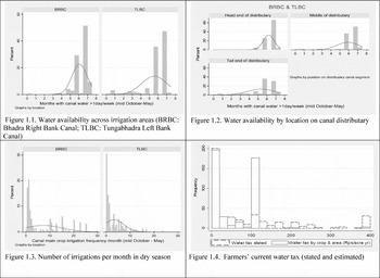
Our sample does not represent the whole of the Bhadra and Tungabhadra command areas, but still reveals the large variation in local irrigation conditions. Average water availability in the upstream Bhadra Right Bank Canal (BRBC) is higher than in the downstream Tungabhadra Left Bank Canal (TLBC) (figure 1.1). Along the largest distributaries in both areas there was a larger proportion of farms with very low water availability in the TLBC than BRBC. Water availability in farms close to the head reach of the distributaries versus middle- and tail-end reaches in both BRBC and TLBC also varies greatly (figure 1.2). Within the sub-minor canals off the main distributary there is clearly also large variation – head reaches have on average one month longer of available water than the tail end, with much wider variation in the tail end than the head end. The main water use conflict of interest lies in overuse of water by head-end farmers relative to tail-end farmers in the Rabi (dry) season. Closer inspection of the dataFootnote 2 shows that the differences between head- and tail-end farmers’ water availability in the dry season is larger in Tungabhadra than in Bhadra.
Inspection of farmer characteristics (not reported here) reveal some other significant patterns across the command areas. Farmers who were Water User Association (WUA) members were found significantly more in areas without the traditional ‘warabundi’ water sharing arrangements. WUA members were more likely to farm arrica nuts than other types of crops (in the Bhadra command area). WUA members were also significantly more likely to be found in middle reaches of distributaries than in head or tail reaches. An interesting hypothesis that must be addressed elsewhere is that there is a water availability interval at which farmers perceive the benefits of formal irrigation organisation to outweigh the costs (Ostrom, Reference Ostrom1990). We looked at a number of other farm characteristics simultaneously to find correlations with WUA membership, but found no other significant relationships (e.g., total cropping area, land holding, other crop types). Where do farmers themselves say they participate in warabundi water sharing systems? These sharing arrangements were significantly more prevalent in tail-end reaches of the distributary than mid- or head-end reaches. This suggests that WUAs are not a necessary condition for warabundi systems or vice versa.
There is a large variation in the number of irrigations/waterings, or actual water use, across the Bhadra and Tungabhadra command areas where we conducted the surveys (figure 1.3). The variation in water use across the area we surveyed is striking: 52.6 per cent of farmers irrigated their crops less than two times a month in the sample, while 24.6 per cent irrigated their crops more than 8 times a month in the dry season (referred to as ‘Rabi’ running mid-October to end of May in this area). The average number of waterings is significantly higher in the Bhadra command. In the Bhadra area some farmers irrigated crops more than 20 times per month whereas this was hardly ever the case in Tungabhadra. Farmers that rely wholly on non-irrigated crops, or do not farm in the dry season, represent more than 30 per cent in Tungabhadra, while less than 20 per cent in Bhadra. Only 9 per cent of farmers who had no dry season crop also stated that they did not water their fields – this means that a significant minority of farmers water their parcels with or without crops.Footnote 3
Farmers in informal warabundi water sharing systems were significantly less likely to have paid their water tax since 2007. Of a total of 432 farmers interviewed, 197 farmers had no cropped area in the dry season, and 167 had not paid water taxes in the 2007–2008 dry season. Average current water tax payment per acre varies according to cropping composition. Farmers’ stated water taxes were somewhat higher than those estimated based on their cropping pattern. Five per cent of the sample stated they paid higher water taxes than the highest official rate (not shown in figure 1.4).
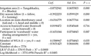
In 66 per cent of choice situations in the CE farmers preferred the current situation to the alternative water regime. Utilizing information about the SQ was therefore key to understanding the majority of farmers’ preferences for their current situation. A simple logit of the probability of selecting the SQ based on some of the sample characteristics described above illustrates possible respondent heterogeneity that may go unobserved if individual baseline SQ is not recorded (table 1). Irrigation canal water availability strongly determines whether farmers choose the SQ, with both the downstream Tungabhadra irrigation command, and location at tail-end of main distributary significantly decreasing probability of choosing SQ. Institutional arrangements also seem to play a role in preference for the SQ, although this may also be a result of water management institutions being endogenous to the level of water supply (see above); membership in a WUA increases the likelihood of preferring the SQ, while participation in warabundi arrangements decreases the probability of preferring SQ.
Logistic regression of some respondent characteristics affecting choice of status quo

4. Methods and materials
4.1. Choice experiment models and estimation
Conditional and mixed logit models are by now well known in the literature and we omit the technical details here. We refer to the general specification for mixed logit model (Revelt and Train, Reference Revelt and Train1998) which is analogous to the way the conditional logit command is used to fit a multinomial logit model in STATA (Hole, Reference Hole2007a). The log likelihood for the mixed logit model cannot be solved analytically so it is approximated using simulation methods (Train, Reference Train2003). We used the ‘mixlogit’ command programmed for STATA by Hole (Reference Hole2007a), which uses simulation based on Halton sequences for the integration (Haan and Uhlendorff, Reference Haan and Uhlendorff2006).
Conditional logit (McFadden, Reference McFadden and Zarembka1974; Chamberlain, Reference Chamberlain1980) with non-random parameters is a special case of the mixed logit model with random parameters when the variance of random parameters is not significantly different from zero (Train, Reference Train2003). In this case the Independence of Irrelevant Alternatives (IIA) assumption of the non-random parameters specification is not rejected and conditional logit may still be unbiased. The conditional logit model also seems to be robust to misspecification and can capture average tastes well even when tastes are random (Train, Reference Train2003). With relatively small data sets the mixed logit simulation model may also have trouble converging on a solution, in which case one must fall back on conditional logit. Small sample stated preference studies will probably be the norm if they are ever to be used outside the research context for water price policy analysis in any given irrigation command area. For the above reasons we have tried to use mixed logit specification where the data permit, falling back on the conditional logit model when discussing the more data demanding models with a non-linear, or effects coded, attribute specification (Hensher et al., Reference Hensher, Rose and Greene2005a).
In the following, we distinguish willingness-to-pay (compensating surplus) of non-marginal improvements of bundles of irrigation water characteristics due to a policy, from the implicit price of marginal improvements in any one attribute. We assume that utility is linear in the attributes of alternatives:

where β 0i is a constant which reflects the mean impact of unobservable components of utility of alternative i, β 1, . . . βK are the coefficients for attributes X 1njt . . . XKnjt and βC is the coefficient for the cost of alternatives (irrigation water charge). Attributes and their levels are shown in table 1.
The marginal value, or implicit price (IP), for an improvement in a specific attribute Xk is found by solving for dC/dXk:

In the calculation of the confidence bounds for IPk, in small sample situations an advantage of the conditional logit model with non-random parameters, over mixed logit with random parameters, is that it can be combined with non-parametric bootstrapping. Non-parametric bootstrapping, although more robust for small samples with unobserved heterogeneity, is not practical to implement in a simulation-based method such as mixed logit because of computation time. Hole (Reference Hole2007b) tested the small sample properties of the delta, Fieller, Krinsky–Robb and bootstrap methods, finding that all the methods produce fairly similar confidence intervals. In order to compute WTP confidence intervals for both the conditional and mixed logit models in a consistent manner, we therefore used the Krinsky–Robb method (Krinsky and Robb, Reference Krinsky and Robb1986, Reference Krinsky and Robb1990), also known as the parametric bootstrap (Efron and Tibshirani, Reference Efron and Tibshirani1993).
4.2. Survey design
Figure A3Footnote 4 shows an example of how a water management scenario was presented to the farmers. Six such choice situations were presented to each farmer, divided into 4 blocks, for a total of 24 different paired choice sets. The 48 choice situations were constructed from a partial factorial design.Footnote 5
The survey instrument was developed in a pilot study carried out in an irrigation area in an adjacent catchment to the present study area (India PES Project, 2008). Because of time constraints pre-testing of the choice cards was conducted in selected sites across the Tungabhadra command area, one of the two irrigation areas in the present study. In retrospect we found that attribute levels selected for the experimental design covered only some of the variation in water supply situations experienced in the Tungabhadra catchment. In head-end reaches farmers often had more water than what was shown in the choice cards, while in tail-end reaches they often had less. Annual water taxes paid were sometimes higher than the totals shown, sometimes less. However, the farm heterogeneity uncovered in the main survey was recorded by first asking farmers to draw their crop sowing, watering frequency per month and harvesting periods on a crop calendar (June–May) similar to the background in the choice cards (figure A3). Information on irrigation canal characteristics was also collected to approximate the volume of a single irrigation on the particular farm. This gave us information about the farmer's current water use situation by crop.
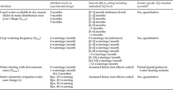
Farmers were then asked to choose between two experimentally generated alternative scenarios and the SQ situation the farmer had hand-drawn earlier on in the survey. In the CE, the same calendar background was used to illustrate hypothetical months of water availability in the canal nearest to the farmer. Attribute levels were illustrated using a green bar with a rice plant icon. This indicated times of year when irrigation could take place. The amount of water available was illustrated by the number of watering/irrigations per month the farmer would have access to in a water sharing system (locally known as warabundi). The concept of water sharing for other needs, particularly for environment (a blue bar with fish) and drinking (a tap icon) was made concrete in terms of the farmer either sharing no water, or foregoing one watering per month for two months to these downstream users. Semi-volumetric water pricing was introduced by stating a charge in Rupees (Rps)/acre/watering, and showing the total annual amount in Rps/acre that this would equal given the number of waterings in the scenario. In this way the farmer could directly relate the annual water charge to what he was currently paying in annual water tax. The characteristic of the hypothetical water regime we asked them to consider is that the annual water charge is now proportional to the number of waterings and months of available water, i.e., more directly related to the volume of water used (semi-volumetric). The height of the green irrigation water charge bar in the calendar was proportional to the charge per watering. Respondents were also asked their payment history of the water tax, socio-economic household and opinion questions. Table 2 summarises the attributes and their levels.
Attributes and levels used in the choice experiment. Note: individual farmer SQ levels could take any value (not limited to the attribute levels of the experimental design)

4.3. Specific interpretations of the irrigation water charge attribute
The irrigation water charge attribute Rps/watering (cjt) was nearly orthogonally distributed in the experimental design (Spearman's rank correlation coefficients relative to cjt are ρfreq = −0.0323(p = 0.02), ρavail = −0.0662(p = 0.000), ρshare = 0.0012(p = 0.931)). A conversion was conducted in order to model a water charge per year per acre that could be directly compared to the current water taxes paid by farmers (as shown in figure A3). The total annual per acre water charges shown in the choice cards was calculated using the following formula:Footnote 6

We would use Cjt if we believe that farmers focus on the annual water charge per acre in the choice cards. The draw-back of using the annual water charge per acre Cjt in the model is that it introduces correlation between attributes (Spearman's rank correlation coefficients relative to Cjt are ρfreq = 0.6357(0.000), ρavail = 0.4737(0.000, ρshare = −0.2606(0.000)). If on the other hand we believe respondents focused on the semi-volumetric water charge we would estimate the model using cjt. Under this specification we would have to convert the SQ attribute levels from the annual water tax farmers stated they currently pay, to an equivalent charge per watering:

where i sq is the SQ level of respondent i.
In other words, in order to implement our model with individual SQ information we cannot avoid the correlation between the attributes of water supply (availability, frequency) and price attributes. We chose to estimate the models with the annual water tax equivalent, Cjt, which we believe is the interpretation most familiar to farmers.. To account for lack of orthogonality we use a mixlogit model allowing for correlation across attributes (Hole, Reference Hole2007a).
4.4. Coding the individual status quo situation
In our CE respondents chose between two unlabelled alternative irrigation water scenarios and a labelled SQ alternative. When the SQ alternative is chosen, we code it with the farm-specific water supply attribute levels, rather than a coding that is invariant across respondents. Coding individual SQ captures information about respondents whose current situation lies within the range of the CEs attribute levels, but also describes those that lie below or above the attribute range. As suggested, this is particularly useful if the pilot survey has failed to adjust attribute level ranges to the heterogeneity of the population. It provides a way of capturing some of the otherwise unobserved heterogeneity in the sample. We do not include an alternative specific constant for the SQ in any of the choice models reported here because it is by definition highly correlated with the individual SQ attribute levels, leading to inflated standard errors of coefficients.
Effects or dummy coding attribute levels can uncover non-linearities in marginal WTP for attributes (implicit prices). Effects coding is a challenge in a model with individual SQ information, because we cannot directly assign an individual's SQ level to the attribute levels, or ‘effects’, given in the experimental design. In a standard approach, each effect usually corresponds to the different exact attribute levels of the experiment (Hensher et al., 2005). In our study, respondents’ individual SQ may take any value bounded below at zero/none and above by the highest water tax currently paid (400 Rps./acre year), total months of dry season (7.5 months), number of days in which an irrigation can take place (30 days/month) and sharing practice (yes).
An effects coded model using only the experimental design attribute levels must drop all the SQ choice observations because they are apparently unknown. In our study this would have meant dropping 66 per cent of our choice information (equal to the SQ response per cent of the total choice alternatives). Using individual SQ information in the effects coding models required interval coding, so that individual SQ and experimental design levels could be described on the same attribute scale. This amounts to assuming that respondents interpreted attribute levels in the design alternatives as midpoint in a range. In continuation we call this an ‘interval effects coding’ (see table 2). An ‘interval effects’ interpretation loses information regarding the effects of the experimental design, but gains information on the individual farmers’ interpretation of their SQ choices. We use the effects coded models for a richer evaluation of whether water availability and watering frequencies are non-linear attributes, and the significance of individual SQ situations outside the particular attribute levels of the experiment.
5. Results
The information in figure 1 leads us initially to hypothesize that unobserved heterogeneity regarding water availability might be normally distributed, watering frequency lognormally distributed and water charge lognormally distributed. Water sharing is a dummy variable and was defined as a fixed variable in the choice models. Model testing revealed that both lognormal and normal specifications of the water charge attribute had about the same significance level.Footnote 7 In addition, the lognormal specification did not converge in the smallest dataset. We therefore run all the mixed logit models with a normal distribution on the random parameters.Footnote 8
Heterogeneity in farmer SQ situations

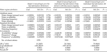
In this study information about the SQ is crucial for fitting a choice model. In the majority of choice situations (66 per cent) farmers preferred the current situation to the alternative water regime. Table 3 shows the effect of including information on the individual SQ, and the difference between models for farmers currently cropping (45.6 per cent), and farmers with fallow land (56.4 per cent) in the 2007–2008 ‘Rabi’ season. Not using the individual SQ information, or excluding non-cropping farmers, severely limits the useful sample size and model significance. In Model 3 we see some significant correlation between attributes selected in the mixed logit.
Significance of including individual SQ information and attribute correlation

Note: Pseudo R2 models 1–3 are not directly comparable – different sample sizes mean they do not belong to the same nested model.
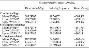
Table 4 shows that the conditional logit model estimates significantly higher implicit prices than the mixed logit model (Model 3 of all farmers). Using Model 2 of dry season crop farmers only we found that conditional logitFootnote 9 and mixed logit implicit price estimates were not significantly different. In other words, farmers who do not currently cultivate in the dry season have a significant effect on estimation of implicit price of irrigation water, and are an important, but easily neglected, group to consider when designing the new water regime.
Attribute implicit prices across model specifications

Note: Calculated using model 3 (all farmers).
Table 4 also shows that accounting for correlation between attributes found in Model 3 does not significantly affect calculation of implicit prices. In other words, the correlation introduced by equation (3.1) does not have a significant effect on welfare estimates. This is probably because correlation introduced in the experimental design is mitigated by the large heterogeneity of the individual SQ attribute levels.
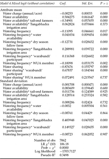
Model 4 with interactions shows both the significant observed, as well as unobserved, heterogeneity in the sample (table 5). Implicit prices for water availability and watering frequency across irrigation areas, canal locations and farm types displays significant variation.Footnote 10
Mixed logit with interaction effects

Note: All farmers, using individual SQ levels and calculated annual water charge (Ci sq) as in Model 3.
We also ‘interval effects coded’ the model to assess possible non-linearity of utility of water availability and watering frequency. Using the range of the individual SQ data we found utility to be non-linear, especially outside the range of the attributes in the experimental design (table A1, figures A4–A5).Footnote 11 The effects coded model illustrates the bias introduced by insufficient range of attribute levels in the CE relative to the full variation of irrigation water conditions experienced by farmers across the sample.
6. Conclusions
This paper has argued that CEs can be used with success to evaluate the wide differences in water availability, farmer practices and preferences that are found in large irrigation command areas such as the Tungabhadra sub-basin in Karnataka, India. By a detailed accounting of farmers’ current situation, and how it affects their preferences for hypothetical water regimes and irrigation prices, we can get a sense of how different segments of the farmer population will react to different hypothetical water supply and pricing regimes. We also showed how CEs could be used to evaluate the WTP for water in different parts of the dry season and for higher irrigation frequency.
Despite care in design and intensive testing of the survey, the pilot sample was not geographically extensive enough to capture the variation in water use practices across the Bhadra and Tungabhadra basins. The CE did not offer a large enough variation in irrigation frequencies to cover the huge variation seen across the two command areas. Consequently, a large proportion of the farmers in water abundant Bhadra felt the water regimes on offer were too frugal and chose the SQ. The use of a CE models that considered individual SQ characteristics of farmers was therefore crucial to evaluating the water availability thresholds at which WTP becomes positive.
In terms of methodological improvements to CEs, we show that accounting for each farmer's individual SQ situation in the choice models improves the explanatory power of models. The CE with individual SQ information is particularly useful in study settings where: (i) one cannot afford to have a large sample, (ii) there is large heterogeneity in use or perception of (environmental) service levels across respondents and (iii) the policy is viewed as so contentious that a significant portion of respondents is expected to prefer their current situation to a proposed policy.