2. Problem formulation

We consider a complete filtered probability space $(\Omega, {\mathcal{F}}, ({\mathcal{F}}_t)_{t\ge 0}, \textrm{P})$ , equipped with a standard Brownian motion $W\coloneqq(W_t)_{t\ge 0}$ . With no loss of generality we assume that $({\mathcal{F}}_t)_{t\ge 0}$ is the filtration generated by W and augmented with $\textrm{P}$ -null sets. Further, we denote by $X\coloneqq(X_t)_{t\in[0, 1]}$ a Brownian bridge pinned at zero at time $T=1$ , i.e. such that $X_1=0$ . If the Brownian bridge starts at time $t\in[0, 1)$ from a point $x\in{\mathbb{R}}$ , we sometimes denote it by $(X^{t,x}_{s})_{s\in[t,1]}$ in order to keep track of the initial condition.

It is well known that, given an initial condition $X_t=x$ at time $t\in[0, 1)$ , the dynamics of X can be described by the following stochastic differential equation (SDE):

(1) \begin{align}{\textrm{d}} X_s=-\frac{X_s}{1-s}{\textrm{d}} s+{\textrm{d}} W_s, \qquad s\in[t,1).\end{align}

The unique strong solution of the SDE (1) is given by

(2) \begin{align}X^{t,x}_s &=(1-s)\bigg(\frac{x}{1-t}+\int_t^s \frac{\textrm{d} W_u}{1-u} \bigg), \qquad s\in[t,1].\end{align}

The expression in (2) allows us to identify (in law) the process $X^{t,x}$ with the process $Z^{t,x}\coloneqq(Z^{t,x}_s)_{s\in[t,1]}$ given by

(3) \begin{equation}Z^{t,x}_s\coloneqq\frac{1-s}{1-t}x+\sqrt{\frac{1-s}{1-t}}W_{s-t}, \qquad s\in[t,1].\end{equation}

That is, we have

(4) \begin{align}\mathsf{Law}\big(X^{t,x}_s,\, s\in[t,1]\big)=\mathsf{Law}\big(Z^{t,x}_s,\,s\in[t,1]\big)\end{align}

for any initial condition $(t,x)\in[0, 1]\times{\mathbb{R}}$ . In the rest of the paper we will often use the notations $\textrm{E}_{t,x}[\!\cdot\!]=\textrm{E}[\,\cdot \mid X_t=x]$ and, equivalently, $\textrm{E}_{t,x}[\!\cdot\!]=\textrm{E}[\,\cdot \mid Z_t=x]$ .

Using the abovementioned identity in law of X and Z, along with well-known distributional properties of the Brownian motion, it can be easily checked that

(5) \begin{align}\textrm{E}_{t,x}\bigg[\sup_{t\leq s\leq 1}{\textrm{e}}^{X_s}\bigg]\le {\textrm{e}}^{|x|}\textrm{E}\big[{\textrm{e}}^{S_1}\big]<+\infty,\end{align}

where $S_1\coloneqq\sup_{0\le s\le 1}|W_s|$ . The random variable $S_1$ will be used several times in what follows, and we denote

(6) \begin{align}c_1\coloneqq\textrm{E}\big[{\textrm{e}}^{S_1}\big]\quad\text{and}\quad c_2\coloneqq\textrm{E}\big[S_1{\textrm{e}}^{S_1}\big].\end{align}

2.1. The stopping problem

Our objective is to study the optimal stopping problem

(7) \begin{equation}v(t,x)=\sup_{0\leq \tau\leq 1-t} \textrm{E}_{t,x}\big[{\textrm{e}}^{X_{t+\tau}}\big] \quad \text{for $(t,x)\in[0, 1]\times{\mathbb{R}}$},\end{equation}

where $\tau$ is a random time such that $t+\tau$ is an $({\mathcal{F}}_s)_{s\geq t}$ -stopping time (in what follows we simply say that $\tau$ is an $({\mathcal{F}}_s)_{s\geq t}$ -stopping time, as no confusion shall arise). Thanks to (5), we can rely upon standard optimal stopping theory to give some initial results. In particular, we split the state space $[0, 1]\times{\mathbb{R}}$ into a continuation region ${\mathcal{C}}$ and a stopping region ${\mathcal{D}}$ , respectively given by

(8) \begin{align}&{\mathcal{C}}\coloneqq\{(t,x)\in[0, 1]\times{\mathbb{R}}\,:\,v(t,x)>{\textrm{e}}^x\},\end{align}

(9) \begin{align} &{\mathcal{D}}\coloneqq\{(t,x)\in[0, 1]\times{\mathbb{R}}\,:\,v(t,x)={\textrm{e}}^x\}.\end{align}

Then, for any $(t,x)\in[0, 1]\times{\mathbb{R}}$ , the smallest optimal stopping time for problem (7) is given by (see, e.g., [Reference Karatzas and Shreve18, Theorem D.12, Appendix D])

(10) \begin{equation}\tau^*\coloneqq\inf\{s\in [0, 1-t]\,:\,(t+s,X_{t+s})\in {\mathcal{D}}\},\qquad \textrm{P}_{t,x}\text{-almost surely (a.s.).}\end{equation}

We will sometimes use the notation $\tau^*_{t,x}$ to keep track of the initial condition of the time-space process (t, X).

Moreover, standard theory on the Snell envelope also guarantees (see, e.g., [Reference Karatzas and Shreve18, Theorem D.9, Appendix D]) that the process $V\coloneqq(V_t)_{t\in[0, 1]}$ defined by $V_t\coloneqq v(t,X_t)$ is a right-continuous, non-negative, $\textrm{P}$ -super-martingale and that $V^*\coloneqq(V_{t\wedge\tau^*})_{t\in[0, 1]}$ is a right-continuous, non-negative, $\textrm{P}$ -martingale.

To conclude this section, we show two further formulations of problem (7) that will become useful in our analysis. The former uses (4) and the fact that, thanks to the above discussion, we only need to look for optimal stopping times in the class of entry times to measurable sets. Hence, we have

(11) \begin{equation}v(t,x)=\sup_{0\leq \tau\leq 1-t} \textrm{E}_{t,x}\big[{\textrm{e}}^{Z_{t+\tau}}\big] \qquad\text{for $(t,x)\in[0, 1]\times{\mathbb{R}}$}.\end{equation}

The second formulation instead uses ideas originally contained in [Reference Jaillet, Lamberton and Lapeyre16]. In particular, for any fixed $t\in[0, 1]$ and any $({\mathcal{F}}_s)_{s\ge t}$ -stopping time $\tau\in[0, 1-t]$ , we can define an $(\hat{{\mathcal{F}}}_s)_{0\leq s\leq 1}$ stopping time $\theta\in[0, 1]$ such that $\tau=\theta(1-t)$ and $\hat{{\mathcal{F}}}_s={\mathcal{F}}_{t+s(1-t)}$ . In addition to this, notice that

\begin{align*} \mathsf{Law}\big(W_{s(1-t)},\, s\ge0\big)=\mathsf{Law}\big(\sqrt{1-t} \, W_s,\,s\ge0 \big).\end{align*}

Therefore, problem (11) (hence problem (7)) can be rewritten as

(12) \begin{equation}v(t,x)=\sup_{0\leq \theta\leq 1} \textrm{E}\big[\exp\big((1-\theta)x+\sqrt{(1-\theta)(1-t)}W_\theta\big)\big].\end{equation}

This last formulation of the problem has the advantage that the domain of admissible stopping times $\theta$ is independent of the initial time t.

Remark 1. There is no loss of generality in our choice of a pinning time $T=1$ and a pinning point $\alpha=0$ . We could equivalently choose a generic pinning time $T>t\geq 0$ and a generic pinning point $\alpha\in{\mathbb{R}}$ and consider the dynamics

\begin{align*}{\textrm{d}} X_s=-\frac{X_s-\alpha}{T-s}{\textrm{d}} s+{\textrm{d}} W_s, \qquad s\in[t,T).\end{align*}

Then, the analysis in the next sections would remain valid up to obvious tweaks.

3. Continuity of the value function and existence of a boundary

In this section we prove some properties of the value function, including its continuity, and derive the existence of a unique optimal stopping boundary. It follows immediately from (5) that the value function is non-negative and uniformly bounded on compact sets. In particular, we have

(13) \begin{align} 0\leq v(t,x)\leq c_1 {\textrm{e}}^{|x|} \qquad \text{for all $(t,x)\in [0, 1]\times {\mathbb{R}}$}, \end{align}

where $c_1>0$ is given by (6).

Proposition 1. The map $x\mapsto v(t,x)$ is convex and non-decreasing. Moreover, for any compact set $K\subset {\mathbb{R}}$ there exists $L_K>0$ such that

\[\sup_{t\in[0, 1]}|v(t,y)-v(t,x)|\leq L_K|y-x| \qquad \text{for all $x,y\in K$.}\]

Proof. The convexity of $x\mapsto v(t,x)$ follows from the linearity of $x\mapsto Z^{t,x}_s$ (see (3)), the convexity of the map $x\mapsto {\textrm{e}}^x$ , and the well-known inequality $\sup(a+b)\le \sup a+\sup b$ .

Monotonicity can be easily deduced by, e.g., the explicit dependence of (12) on $x\in{\mathbb{R}}$ . As for the Lipschitz continuity, the claim is trivial for $t=1$ since $v(1,x)=\textrm{e}^x$ . For the remaining cases, fix $t\in[0, 1)$ and let us fix $y\geq x$ . Denote $\tau_y\coloneqq\tau^*_{t,y}$ , then by the monotonicity of $v(t,\,\cdot\,)$ , the fact that $\tau_y$ is sub-optimal for v(t, x), and simple estimates, we obtain

\begin{align*} 0 & \leq v(t,y)-v(t,x) \\[3pt] &\leq \textrm{E}\big[{\textrm{e}}^{Z^{t,y}_{t+\tau_y}}-{\textrm{e}}^{Z^{t,x}_{t+\tau_y}}\big] \\[3pt] & = \textrm{E}\bigg[\bigg(\exp\bigg(\frac{1-(t+\tau_y)}{1-t}y\bigg)-\exp\bigg(\frac{1-(t+\tau_y)}{1-t}x\bigg)\bigg)\exp\bigg(\sqrt{\frac{1-(t+\tau_y)}{1-t}}W_{\tau_y}\bigg)\bigg]\\[3pt] &\le \textrm{E}\bigg[\bigg(\frac{1-(t+\tau_y)}{1-t}\bigg)\exp\bigg(\sqrt{\frac{1-(t+\tau_y)}{1-t}}W_{\tau_y}\bigg)\bigg]{\textrm{e}}^{|x|\vee |y|}(y-x)\\[3pt] &\le \textrm{E}\big[{\textrm{e}}^{S_1}\big]{\textrm{e}}^{|x|\vee |y|}(y-x). \end{align*}

Hence, the claim follows with $L_K\coloneqq c_1 \max_{x\in K}\textrm{e}^{|x|}$ . □

Next, we show that the value function is locally Lipschitz in time on $[0, 1)\times{\mathbb{R}}$ . However, it fails to be continuous at $\{1\}\times(-\infty,0)$ .

Proposition 2. For any $T<1$ and any $0\le t_1<t_2\le T$ , we have

(14) \begin{align}|v(t_2,x)-v(t_1,x)|\leq \frac{c_2\textrm{e}^{|x|}}{2\sqrt{1-T}}(t_2-t_1) \qquad \textit{for $x\in{\mathbb{R}}$},\end{align}

with $c_2>0$ as in (6). Moreover,

(15) \begin{align}&\lim_{t\to 1}v(t,x)=\textrm{e}^x\qquad\qquad\quad for\, x\ge 0,\end{align}

(16) \begin{align}&\liminf_{t\to 1}v(t,x)\ge 1> \textrm{e}^x \qquad for\, x < 0.\end{align}

Proof. For the proof of (14) we will refer to the problem formulation in (12). Fix $0\leq t_1<t_2\leq T<1$ and let $\theta_2\coloneqq\theta^*_{t_2,x}$ be the optimal stopping time for $v(t_2,x)$ . Then, given that $\theta_2$ is admissible and sub-optimal for the problem with value $v(t_1,x)$ , we have

(17) \begin{align} &v(t_2,x)-v(t_1,x)\\[3pt] &\quad \leq \textrm{E}\big[{\textrm{e}}^{(1-\theta_2)x} \big({\textrm{e}}^{\sqrt{(1-\theta_2)(1-t_2)}W_{\theta_2}}-{\textrm{e}}^{\sqrt{(1-\theta_2)(1-t_1)}W_{\theta_2}}\big)\big]\notag\\[3pt] &\quad \leq {\textrm{e}}^{|x|}\textrm{E}\big[{\textrm{e}}^{\sqrt{(1-\theta_2)(1-t_1)}|W_{\theta_2}|}\sqrt{(1-\theta_2)}|W_{\theta_2}|\big]\big(\sqrt{1-t_1}-\sqrt{1-t_2}\big)\notag\\[3pt] &\quad \leq {\textrm{e}}^{|x|}\textrm{E}\big[S_1{\textrm{e}}^{S_1}\big]\frac{t_2-t_1}{2\sqrt{1-T}}.\notag \end{align}

Now, setting $\theta_1\coloneqq\theta^*_{t_1,x}$ we notice that $\theta_1$ is admissible and sub-optimal for the problem with value $v(t_2,x)$ . Then, arguments as above give

\[v(t_2,x)-v(t_1,x)\geq -{\textrm{e}}^{|x|}\textrm{E}\big[S_1{\textrm{e}}^{S_1}\big]\frac{t_2-t_1}{2\sqrt{1-T}},\]

which, combined with (17), implies (14).

Finally, we show (15) and (16). Notice first that $v(1,x)=\textrm{e}^x$ and $v(t,x)\geq {\textrm{e}}^x$ for $t\in[0, 1)$ . Pick $x\geq 0$ , then by (11) we have ${\textrm{e}}^x\leq v(t,x)\leq {\textrm{e}}^x\textrm{E}\left[e^{S_{1-t}}\right]$ , which implies (15) by dominated convergence and using that $S_{1-t}\to0$ as $t\to 1$ . If $x<0$ instead, the sub-optimal strategy $\tau=1-t$ gives $v(t,x)\geq 1$ . Hence, $\liminf_{t\to 1} v(t,x)\geq 1> {\textrm{e}}^x=v(1,x)$ as in (16). □

As a corollary of the two propositions just stated, we have that ${\mathcal{C}}$ is an open set. Combining this fact with the martingale property (in ${\mathcal{C}}$ ) of the value function, we obtain that $v\in C^{1,2}({\mathcal{C}})$ and it solves the free boundary problem (see, e.g., arguments as in the proof of Theorem 7.7 in Chapter 2, Section 7 of [Reference Karatzas and Shreve18])

(18) \begin{align}\big(\partial_t +\tfrac{1}{2}\partial_{xx}-\tfrac{x}{1-t}\partial_x\big) v(t,x) &= 0,\qquad\ (t,x)\in{\mathcal{C}},\end{align}

(19) \begin{align} v(t,x) &= {\textrm{e}}^x\qquad\ \ (t,x)\in\partial{\mathcal{C}},\end{align}

where $\partial_t$ , $\partial_x$ , and $\partial_{xx}$ denote the time derivative, the first spatial derivative, and the second spatial derivative, respectively.

For future reference, we also denote by ${\mathcal{L}}$ the second-order differential operator associated with X. That is,

\begin{align*} ({\mathcal{L}} f)(t,x)\coloneqq\dfrac{1}{2}\partial_{xx}\,f(t,x)-\dfrac{x}{1-t}\partial_x\,f(t,x) \qquad\text{for any $f\in C^{0,2}({\mathbb{R}}^2)$}.\end{align*}

3.1. Existence of an optimal boundary

In order to prove the existence of an optimal boundary it is convenient to perform a change of measure in our problem formulation (7). In particular, using the integral form of (1) (upon setting $B_\tau\coloneqq W_{t+\tau}-W_t$ ), we have

\begin{align*}\textrm{E}\left[\exp(X^{t,x}_{t+\tau})\right] &= \textrm{E}\bigg[\exp\bigg(x+B_\tau-\int_0^\tau\frac{X^{t,x}_{t+s}}{1-(t+s)}\, \textrm{d} s\bigg)\bigg] \\[3pt] &= {\textrm{e}}^x\textrm{E}\bigg[\exp\big(B_\tau-\frac 1 2 \tau\big)\exp\bigg(\int_0^\tau \bigg(\frac 1 2 -\frac{X^{t,x}_{t+s}}{1-(t+s)}\bigg)\textrm{d} s\bigg)\bigg]\\[3pt] &={\textrm{e}}^x{\widetilde{\textrm{E}}}\bigg[\exp\bigg(\int_0^\tau \bigg(\frac 1 2 -\frac{X^{t,x}_{t+s}}{1-(t+s)}\bigg)\textrm{d} s\bigg)\bigg],\end{align*}

where

\[\frac{{\textrm{d}}{\widetilde{\textrm{P}}}}{{\textrm{d}}\textrm{P}}\bigg|_{{\mathcal{F}}_{1}}\coloneqq\exp\bigg(B_{1-t}-\frac {1} {2} (1-t)\bigg) \]

defines a new equivalent probability measure ${\widetilde{\textrm{P}}}$ on ${(\Omega,{\mathcal{F}})}$ and the associated expected value ${\widetilde{\textrm{E}}}$ . Under ${\widetilde{\textrm{P}}}$ , we have

\begin{align*} {\textrm{d}} X^{t,x}_s=\left(1-\frac{X^{t,x}_s}{1-s}\right)\textrm{d} s+\textrm{d} \widetilde{W}_s \qquad\text{for $s\in[t,1]$},\end{align*}

with $X^{t,x}_t=x$ , and with $\widetilde W_t\coloneqq W_t-t$ defining a ${\widetilde{\textrm{P}}}$ -Brownian motion by Girsanov’s theorem.

Thanks to this transformation of the expected payoff, it is clear that solving problem (7) is equivalent to solving

(20) \begin{equation}\tilde{v}(t,x)\coloneqq\sup_{0\leq \tau \leq 1-t}{\widetilde{\textrm{E}}}\bigg[\exp\bigg(\int_0^\tau \bigg(\frac 1 2 -\frac{X^{t,x}_{t+s}}{1-(t+s)}\bigg)\textrm{d} s\bigg)\bigg].\end{equation}

Notice that, indeed, $v(t,x)={\textrm{e}}^x\tilde{v}(t,x)$ implies that

\[{\mathcal{C}}=\{(t,x)\in[0, 1]\times{\mathbb{R}}\,:\,\tilde{v}(t,x)>1\}.\]

Moreover, since V is a $\textrm{P}$ -super-martingale and $V^*$ is a $\textrm{P}$ -martingale then, as a consequence of Girsanov’s theorem, the process $\widetilde{V}\coloneqq(\widetilde{V}_t)_{t\in[0, 1]}$ defined as

(21) \begin{align}\widetilde V_t\coloneqq\exp\left(\int_0^t \left(\frac 1 2 -\frac{X_{s}}{1-s}\right)\textrm{d} s\right)\tilde v(t,X_t)\end{align}

is a ${\widetilde{\textrm{P}}}$ -super-martingale and $\widetilde V^*\coloneqq(\widetilde{V}_{t\wedge\tau^*})_{t\in[0, 1]}$ is a ${\widetilde{\textrm{P}}}$ -martingale, with $\tau^*$ as in (10).

Using this formulation, we can easily obtain the next result.

Proposition 3. There exists a function $b\,:\,[0, 1]\to{\mathbb{R}}_{+} {\cup \{+\infty\}}$ such that

(22) \begin{align}{\mathcal{C}}=\{(t,x)\in[0, 1)\times{\mathbb{R}}\,:\,x<b(t)\}.\end{align}

Proof. Thanks to the pathwise uniqueness of the Brownian bridge, it is clear that for any $x\leq x'$ we have, $\textrm{P}$ -a.s. (hence also ${\widetilde{\textrm{P}}}$ -a.s.),

\[X_s^{t,x}\leq X_s^{t,x'} \qquad \text{for all $s\in[t,1]$}.\]

Using such a comparison principle and (20), it is easy to show that $x\mapsto \tilde{v}(t,x)$ is non-increasing. This means, in particular, that if $(t,x)\in{\mathcal{D}}$ , then $(t,x')\in{\mathcal{D}}$ for all $x'\ge x$ . Then, we define

(23) \begin{align} b(t) &\coloneqq\sup\{x\in{\mathbb{R}}\,:\,\tilde{v}(t,x)>1\}\\[3pt] & \, = \sup\{x\in{\mathbb{R}}\,:\,v(t,x)>{\textrm{e}}^x\}, \qquad t\in[0, 1),\notag \end{align}

and (22) holds by continuity of the value function. For future reference, notice that (23) and (15)–(16) also give $b(1)=0$ .

It remains to show that $b(t)\ge 0$ for all $t\in[0, 1]$ . By choosing the stopping rule $\tau=1-t$ , one has $v(t,x)\geq 1>{\textrm{e}}^x$ for $x<0$ and any $t\in[0, 1)$ . Hence,

\[[0, 1)\times(\!-\infty,0)\subset{\mathcal{C}},\]

and the claim follows. □

As a straightforward consequence of the proposition above and (10), we have

(24) \begin{equation}\tau^*_{t,x}=\inf\{s\in[0, 1-t]\,:\, X^{t,x}_{t+s}\geq b(t+s)\}.\end{equation}

4. Regularity of the optimal boundary

In this section we show that the optimal boundary is monotonic, continuous, and bounded. We will then, in the next section, use these properties to derive smoothness of the value function across the optimal boundary.

By an application of Dynkin’s formula we know that, given any initial condition $(t,x)\in[0, 1)\times{\mathbb{R}}$ , any stopping time $\tau\in[0, 1-t]$ , and a small $\delta>0$ we have

\begin{align*}v(t,x)\ge\textrm{E}_{t,x}\big[{\textrm{e}}^{X_{t+\tau\wedge \delta}}\big]={\textrm{e}}^x+\textrm{E}_{t,x}\bigg[\int_0^{\tau\wedge \delta}{\textrm{e}}^{X_{t+s}}\bigg(\frac{1}{2}-\frac{X_{t+s}}{1-(t+s)}\bigg){\textrm{d}} s\bigg].\end{align*}

This shows that immediate stopping can never be optimal inside the set

(25) \begin{align}{\mathcal{Q}}\coloneqq\left\{(t,x)\in[0, 1)\times{\mathbb{R}}\,:\,x<\dfrac{1}{2} (1-t)\right\},\end{align}

and so ${\mathcal{Q}}\subseteq{\mathcal{C}}$ .

The next result, concerning monotonicity of the optimal boundary, is crucial for the subsequent analysis of the stopping set and of the value function. Monotonicity of optimal boundaries is relatively easy to establish in optimal stopping problems when the underlying diffusion is time homogeneous and the gain function is independent of time. In our case, the latter condition holds but our diffusion is time dependent, hence new ideas are needed in the proof of the theorem below. We also remark that, while in some stopping problems of a Brownian bridge (see, e.g., [Reference Ekström and Wanntorp11]) it is possible to rely upon a time change in order to formulate an auxiliary equivalent stopping problem for a time-homogeneous diffusion (see [Reference Pedersen and Peskir21]), this is not the case here, due to the exponential nature of the gain function.

Proof. It is sufficient to show that, for any fixed $x\in{\mathbb{R}}$ , the map $t\mapsto v(t,x)$ is non-increasing on [0, 1). Indeed, the latter implies monotonicity of the boundary on [0, 1] by definition (23) and using that $b(t)\geq 0$ for all $t\in[0, 1)$ and $b(1)=0$ .

Recalling (18) and using the convexity of $x\mapsto v(t,x)$ , we obtain

\begin{equation*} \partial_t v(t,x)\leq \frac{x}{1-t}\partial_x v(t,x) \qquad \text{for all } (t,x)\in {\mathcal{C}},\end{equation*}

and, in particular,

(26) \begin{align}\partial_t v(t,x)\leq 0 \qquad\text{for all $(t,x)\in[0, 1)\times(-\infty,0]$,}\end{align}

thanks to the fact that ${\mathcal{Q}}\subseteq {\mathcal{C}}$ (see (25)) and $\partial_x v\ge 0$ in ${\mathcal{C}}$ (Proposition 1).

Notice that if $(t,x)\in {\mathcal{D}}\setminus\partial{\mathcal{C}}$ then $v(t,x)={\textrm{e}}^x$ and $\partial_t v(t,x)=0$ . Since $t\mapsto v(t,x)$ is continuous on [0, 1), it only remains to prove that $\partial_t v(t,x)\leq 0$ for $(t,x)\in {\mathcal{C}}$ with $x>0$ . For that, we proceed in two steps.

Step 1. (Property of $t\mapsto X^{t,x}$ ). Consider $(t,x)\in {\mathcal{C}}$ with $x>0$ and $0<{\varepsilon}\leq t<1$ , for some ${\varepsilon}>0$ . For $s\in[0, 1-t]$ we denote

\begin{align*} Y^{t,x;{\varepsilon}}_{t+s}\coloneqq X^{t,x}_{t+s}-X^{t-{\varepsilon},x}_{t-{\varepsilon}+s}.\end{align*}

Since (t, x) is fixed, we simplify the notation and set $Y^{\varepsilon}_{t+s}\coloneqq Y^{t,x;{\varepsilon}}_{t+s}$ , for $s\in[0, 1-t]$ . Next, for some small $\delta>0$ , we let $t_\delta\coloneqq(1-t-\delta)>0$ and $\rho_\delta\coloneqq t_\delta\wedge\tau^0$ , where $\tau^0\coloneqq\tau^0_{t,x}\coloneqq\inf\{u\in[0, 1-t]\,:\,X_{t+u}^{t,x}\leq 0\}$ . Then, using the integral form of (1), for an arbitrary $s\in[0, 1-t]$ we have, $\textrm{P}$ -a.s.,

(27) \begin{align} Y^{\varepsilon}_{t+s\wedge\rho_\delta} &= -\int_0^{s\wedge\rho_\delta} \frac{X^{t,x}_{t+u}}{1-(t+u)}\textrm{d} u+\int_0^{s\wedge\rho_\delta} \frac{X^{t-{\varepsilon},x}_{t-{\varepsilon}+u}}{1-(t-{\varepsilon}+u)}\textrm{d} u\\[9pt] &=-\int_0^{s\wedge\rho_\delta}\bigg( \frac{{\varepsilon} X^{t,x}_{t+u}}{(1-(t-{\varepsilon}+u))(1-(t+u))}+\frac{Y^{{\varepsilon}}_{t+u}}{1-(t-{\varepsilon}+u)}\bigg)\textrm{d} u. \nonumber \end{align}

Let $[x]^+\coloneqq\max\{0,x\}$ . Since $Y^{\varepsilon}$ is a continuous process of bounded variation and $Y^{\varepsilon}_0=0$ , we have

\begin{align*}[Y^{\varepsilon}_{t+s\wedge\rho_\delta}]^+=\int_0^{s\wedge\rho_\delta}{\textbf{1}}_{\{Y^{\varepsilon}_{t+u}\ge 0\}}{\textrm{d}} Y^{\varepsilon}_{t+u}\le 0 ,\end{align*}

where the final inequality follows from (27), upon observing that $X^{t,x}_{t+u}\geq 0$ for all $u\leq\rho_\delta$ . Then, $Y^{{\varepsilon}}_{t+s\wedge \rho_\delta}\leq 0$ for all $s\in[0, 1-t]$ . Furthermore, letting $\delta\to0$ , we obtain, by continuity of paths,

(28) \begin{equation}X^{t-{\varepsilon},x}_{t-{\varepsilon}+s\wedge \tau^0}\geq X^{t,x}_{t+s\wedge \tau^0}\ge 0 \qquad\text{for all } s\in[0, 1-t],\,\,\textrm{P}\text{-a.s.} \end{equation}

Hence, the process $X^{t,x}$ hits zero before the process $X^{t-{\varepsilon},x}$ does.

Step 2. ( $\partial_t v(t,x)\le 0$ ). Fix $(t,x)\in{\mathcal{C}}$ with $x>0$ . Using the same notation as in Step 1 above, let $\sigma\coloneqq\tau^*_{t,x}\wedge \tau^0_{t,x}$ . By the (super-)martingale property of the value function, noticing that $\tau^*$ is optimal in v(t, x) and sub-optimal in $v(t-{\varepsilon},x)$ , we have

(29) \begin{align} & v(t,x)-v(t-{\varepsilon},x)\\[5pt] & \leq \textrm{E}\big[v(t+\sigma,X^{t,x}_{t+\sigma})-v(t-{\varepsilon}+\sigma, X^{t-{\varepsilon},x}_{t-{\varepsilon}+\sigma})\big]\notag \\[5pt] & \leq\textrm{E}\big[{\textbf{1}}_{\{\tau^*\leq\tau^0\}\cap\{\tau^*<1-t\}}(\exp(X^{t,x}_{t+\tau^*})-\exp(X^{t-{\varepsilon},x}_{t-{\varepsilon}+\tau^*}))\big]\notag \\[5pt] & \quad +\textrm{E}\big[{\textbf{1}}_{\{\sigma=1-t\}}(\exp(X^{t,x}_{1})-\exp(X^{t-{\varepsilon},x}_{1-{\varepsilon}}))\big]\notag \\[5pt] & \quad +\textrm{E}\big[{\textbf{1}}_{\{\tau^0<\tau^*\}\cap\{\tau^0<1-t\}}(v(t+\tau^0,0)-v(t-{\varepsilon}+\tau^0,X_{t-{\varepsilon}+\tau^0}^{t-{\varepsilon},x}))\big]. \notag \end{align}

Recalling (28), on the event $\{\tau^*\leq\tau^0\}\cap\{\tau^*<1-t\}$ we have 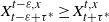$X^{t-{\varepsilon},x}_{t-{\varepsilon}+\tau^*}\geq X^{t,x}_{t+\tau^*}$ , and on the event $\{\sigma=1-t\}$ we have that $X^{t-{\varepsilon},x}_{1-{\varepsilon}}\geq X^{t,x}_{1}$ . Moreover, $x\mapsto v(t,x)$ is non-decreasing (Proposition 1). Thus, combining these facts with (29), we obtain

(30) \begin{align}&v(t,x)-v(t-{\varepsilon},x) \\[5pt] &\leq\textrm{E}\big[{\textbf{1}}_{\{\tau^0<\tau^*\}\cap\{\tau^0<1-t\}}(v(t+\tau^0,0)-v(t-{\varepsilon}+\tau^0,0))\big]\leq 0,\notag \end{align}

where the final inequality uses (26) and the fact that $\tau^0<1-t$ .

Finally, dividing both sides of (30) by ${\varepsilon}$ and letting ${\varepsilon}\to 0$ , we obtain $\partial_t v(t,x)\le 0$ as needed. □

It is well known in optimal stopping theory that monotonicity of the boundary leads to its right continuity (or left continuity). In our case we have a simple corollary.

Proof. Let $t\in[0, 1)$ be such that $b(t)<+\infty$ . Consider a sequence $(t_n)_{n\in {\mathbb{N}}}$ such that $t_n\downarrow t$ as $n\to\infty$ . By monotonicity of b and (22), we have that $b(t_n)<\infty$ and $(t_n,b(t_n))\in {\mathcal{D}}$ for all $n\in {\mathbb{N}}$ . Since ${\mathcal{D}}$ is a closed set and $(t_n,b(t_n))\to (t,b(t+))$ , then also $(t,b(t+))\in {\mathcal{D}}$ (the right limit $b(t+)$ exists by monotonicity). Hence, $b(t+)\geq b(t)$ (see (22)). However, by monotonicity $b(t)\geq b(t+)$ , which leads to $b(t)=b(t+)$ . □

We can now show that the optimal boundary is continuous and bounded on [0, 1].

Proposition 4. The optimal boundary $t\mapsto b(t)$ is continuous on [0, 1] and we have

(31) \begin{equation}\sup_{t\in[0, 1]} b(t)<+\infty.\end{equation}

The proof of Proposition 4 relies upon four lemmas. First we state and prove those lemmas and then we prove the proposition.

Proof. Suppose by contradiction that this is not true and there exists $t\in[0, 1)$ such that ${\mathcal{D}}\cap ([t,1)\times {\mathbb{R}})=\varnothing$ . Then $\tau^*_{t',x}=1-t'$ , $\textrm{P}$ -a.s. for all $(t',x)\in[t,1)\times{\mathbb{R}}$ , which implies $v(t',x)=1$ . This, however, leads to a contradiction since immediate stopping gives $v(t',x)\ge {\textrm{e}}^x>1$ for $x>0$ and any $t'\in[t,1)$ . □

Notice that the lemma above implies that for any $t_1\in[0, 1)$ there exists $t_2\in(t_1,1)$ such that $b(t_2)<+\infty$ . This fact will be used in the next lemma.

Proof. By contradiction, let us assume that there is $t\in(0, 1)$ such that $b(t)=+\infty$ . Then, thanks to Lemma 1 and Corollary 1 we can find $t'\in(t,1)$ such that $0\leq b(t') \eqqcolon b_0<+\infty$ and $(t,t')\times{\mathbb{R}}\subseteq{\mathcal{C}}$ . Let $\sigma_0\coloneqq\inf\{s\in [0, 1-t)\,:\,X_{t+s}^{t,x}\leq b_0\}\wedge (t'-t)$ ; then, recalling $\tau^*_{t,x}$ as in (24), we immediately see that $\textrm{P}(\tau^*_{t,x}\ge \sigma_0)=1$ . Using the martingale property of the value function (see (21)), we obtain

\begin{align*} \tilde{v}(t,x) &= {\widetilde{\textrm{E}}}_{t,x}\left[\exp\left(\int_0^{\sigma_0}\left(\frac 1 2 - \frac {X_{t+s}}{1-(t+s)}\right)\textrm{d} s\right)\tilde{v}(t+\sigma_0,X_{t+\sigma_0})\right]\\[5pt] &= {\widetilde{\textrm{E}}}_{t,x}\left[{\textbf{1}}_{\{\sigma_0 < t'-t\}}\exp\left(\int_0^{\sigma_0}\left(\frac 1 2 - \frac{X_{t+s}}{1-(t+s)}\right)\textrm{d} s\right)\tilde{v}(t+\sigma_0,b_0)\right] \\[5pt] & \quad + {\widetilde{\textrm{E}}}_{t,x}\left[{\textbf{1}}_{\{\sigma_0 = t'-t\}}\exp\left(\int_0^{t'-t}\left(\frac 1 2 - \frac{X_{t+s}}{1-(t+s)}\right)\textrm{d} s\right)\cdot 1 \right], \end{align*}

where we have used continuity of paths and the fact that on $\{\sigma_0=t'-t\}$ it must be $X_{t'}\ge b(t')=b_0$ , ${\widetilde{\textrm{P}}}_{t,x}$ -a.s.

Moreover, since $X_{t+s}^{t,x}\geq b_0$ for $s\leq \sigma_0$ , we have

(32) \begin{align} \tilde{v}(t,x) & \leq {\widetilde{\textrm{E}}}_{t,x}\left[{\textbf{1}}_{\{\sigma_0 < t'-t\}}\exp\left(\int_0^{\sigma_0}\left(\frac 1 2 - \frac{b_0}{1-(t+s)}\right)\textrm{d} s\right)\tilde{v}(t+\sigma_0,b_0)\right]\\[5pt] &\quad+ {\widetilde{\textrm{E}}}_{t,x}\left[{\textbf{1}}_{\{\sigma_0=t'-t \}}\exp\left(\int_0^{t'-t}\left(\frac 1 2 - \frac{X_{t+s}\vee b_0}{1-(t+s)}\right)\textrm{d} s\right) \right]\notag\\[5pt] &\leq {\widetilde{\textrm{E}}}_{t,x}\left[{\textbf{1}}_{\{\sigma_0< t'-t\}}\left(\frac{1-(t+\sigma_0)}{1-t}\right)^{b_0}{\textrm{e}}^{\sigma_0/2} \right]\cdot c_1 \notag\\[5pt] &\quad + {\widetilde{\textrm{E}}}_{t,x}\left[{\textbf{1}}_{\{\sigma_0= t'-t\}}\exp\left(\int_0^{t'-t}\left(\frac 1 2 - \frac{X_{t+s}\vee b_0}{1-(t+s)}\right)\textrm{d} s\right) \right]\notag\\[5pt] &\leq c_1{\textrm{e}}^{1/2}{\widetilde{\textrm{P}}}_{t,x}(\sigma_0 < t'-t)+{\widetilde{\textrm{E}}}\left[\exp\left(\int_0^{t'-t}\left(\frac 1 2 - \frac{X^{t,x}_{t+s}\vee b_0}{1-(t+s)}\right)\textrm{d} s\right) \right],\notag \end{align}

where in the second inequality we have used (13) and $\tilde{v}(t,x)={\textrm{e}}^{-x}v(t,x)$ . Now, we let $x\to\infty$ and notice that

\[{\widetilde{\textrm{P}}}_{t,x}(\sigma_0< t'-t)\le {\widetilde{\textrm{P}}}\big(\inf_{s\in[t,t']}X^{t,x}_s<b_0\big) ,\]

so that the first term on the right-hand side of (32) goes to zero. Similarly, given that $\lim_{x\to\infty} X^{t,x}_{t+s}=+\infty$ for any $s\in[0,t'-t]$ , the second term goes to zero as well by the reverse Fatou lemma. Then, recalling that $\tilde v\ge 1$ , we reach the contradiction

\[ \limsup_{x\to+\infty}\tilde{v}(t,x)\leq 0. \]

It follows that $b(t)<+\infty$ for all $t\in(0, 1]$ since, by definition, $b(1)=0$ . □

Proof. Consider an auxiliary problem where the Brownian bridge is pinned at time $1+h$ , for some $h>0$ , and the time horizon of the optimisation is $1+h$ . That is, let us set

\begin{equation*}v^h(t,x)\coloneqq\sup_{0\leq\tau\leq 1+h-t}\textrm{E}_{t,x}\big[{\textrm{e}}^{\widetilde{X}_{t+\tau}}\big],\end{equation*}

where $\widetilde{X}$ is a Brownian bridge (2) pinned at time $1+h$ .

By the same argument as in Section 2, it follows that $\mathsf{Law}(\widetilde{X}^{t,x})=\mathsf{Law}(\widetilde{Z}^{t,x})$ , where

\[\widetilde{Z}^{t,x}_s=\frac{1+h-s}{1+h-t}x+\sqrt{\frac{1+h-s}{1+h-t}}W_{s-t} \qquad\text{for $s\in[t,1+h]$.}\]

Thus,

(33) \begin{align}v^h(t,x)=\sup_{0\leq\tau\leq 1+h-t}\textrm{E}_{t,x}\big[{\textrm{e}}^{\widetilde{Z}_{t+\tau}}\big]\end{align}

and, since $\mathsf{Law}(Z^{t,x}_s,\,s\in[t,1])=\mathsf{Law}(\widetilde{Z}^{t+h,x}_{s+h},\,s\in[t,1])$ (compare (11) with (33)), we also have that

(34) \begin{align}v(t,x)=v^h(t+h,x) \qquad \text{for all $(t,x)\in[0, 1]\times{\mathbb{R}}$}.\end{align}

By the same arguments as for the original problem, we obtain that there exists a non-decreasing, right-continuous optimal boundary $t\mapsto b^h(t)$ such that

\[{\mathcal{C}}^h\coloneqq\{(t,x)\in[0, 1+h]\times{\mathbb{R}}\,:\,v^h(t,x)>\textrm{e}^x\}=\{(t,x)\in[0, 1+h)\times{\mathbb{R}}\,:\,x<b^h(t)\}.\]

Moreover, since the gain function ${\textrm{e}}^x$ does not depend on time, using (34) we obtain

\[b(t)=b^h(t+h) \qquad \text{for all $t\in[0, 1]$.}\]

In particular, $b(0)=b^h(h)$ and $b^h(h)<+\infty$ by applying the result in Lemma 2 to the auxiliary problem. □

Using ideas as in [Reference De Angelis4], we can also prove left continuity of the optimal boundary.

Proof. We first prove that the boundary is left continuous for all $t\in(0, 1)$ and then that its left limit at $t=1$ is zero, that is $b(1-)=0=b(1)$ .

Suppose, by contradiction, that there exists $t_0\in(0, 1)$ such that $b(t_0-)>b(t_0)$ and consider an interval $[x_1,x_2]\subset (b(t_0),b(t_0-))$ . By monotonicity of b, we have that $[0,t_0)\times[x_1,x_2]\subset {\mathcal{C}}$ . Now, pick an arbitrary, non-negative $\varphi\in{\mathcal{C}}_c^{\infty}([x_1,x_2])$ . Since (18) holds in $[0,t_0)\times[x_1,x_2]$ , then, for any $t<t_0$ , we have

(35) \begin{align} 0 & = \int_{x_1}^{x_2} [\partial_t v(t,y)+{\mathcal{L}} v(t,y)]\varphi(y)\textrm{d} y\\[5pt] &\leq \int_{x_1}^{x_2}{\mathcal{L}} v(t,y) \varphi(y)\textrm{d} y = \int_{x_1}^{x_2} v(t,y) ({\mathcal{L}}^* \varphi)(t,y) \textrm{d} y, \nonumber \end{align}

where for the inequality we have used $\partial_{t}v\le 0$ (see the proof of Theorem 1) and in the final equality we have applied integration by parts and used the adjoint operator

\[ ({\mathcal{L}}^* \varphi)(t,y)\coloneqq\frac 1 2 \varphi''(y)+\frac{1}{1-t}\cdot\frac{{\textrm{d}}}{{\textrm{d}} y}(y\cdot \varphi(y)). \]

Taking limits as $t\to t_0$ and using the dominated convergence theorem, we obtain

(36) \begin{align} 0 & \leq \lim_{t\uparrow t_0} \int_{x_1}^{x_2} v(t,y) ({\mathcal{L}}^* \varphi)(t,y) \textrm{d} y=\int_{x_1}^{x_2} v(t_0,y)({\mathcal{L}}^* \varphi)(t_0,y)\textrm{d} y\\[4pt] &= \int_{x_1}^{x_2} {\textrm{e}}^y ({\mathcal{L}}^* \varphi)(t_0,y) \textrm{d} y = \int_{x_1}^{x_2} {\textrm{e}}^y \left(\frac{1}{2}-\frac{y}{1-t_0} \right) \varphi(y) \textrm{d} y,\nonumber \end{align}

where we have used that $v(t_0,y)={\textrm{e}}^y$ and integration by parts in the final equality.

Finally, recalling that $x_1\geq b(t_0)>\frac{1-t_0}{2}$ , then (36) leads to a contradiction because the right-hand side of the expression is strictly negative (also $\varphi$ is arbitrary).

In order to prove that $b(1-)=b(1)=0$ , we need a slight modification of the argument above. In particular, suppose by contradiction that $b(1-)>0$ and consider an interval $[x_1,x_2]\subset (0,b(1-))$ . Then, replacing $\varphi$ in (35) with $\tilde{\varphi}(t,x)\coloneqq(1-t)\varphi(x)$ , and using the same arguments with $t_0=1$ , we reach a contradiction, i.e.

\begin{equation*} 0\leq \lim_{t\uparrow 1}\int_{x_1}^{x_2} v(t,y)({\mathcal{L}} \tilde{\varphi})(t,y)\textrm{d} y=\int_{x_1}^{x_2} {\textrm{e}}^y\frac{\textrm{d}}{\textrm{d}y}(y\cdot \varphi(y))\textrm{d}y=-\int_{x_1}^{x_2} {\textrm{e}}^y y \varphi(y)\textrm{d}y<0.{\square}\end{equation*}

We are now able to prove Proposition 4.

Proof of Proposition 4. The proof of (31) follows immediately from Lemmas 2 and 3. Right continuity of the boundary follows from Corollary 1 and (31), whereas left continuity follows from Lemma 4. Thus, the optimal boundary is bounded and continuous on [0, 1]. □

5. Regularity of the value function and integral equations

Thanks to the monotonicity of the optimal boundary and to the law of iterated logarithm (combined with (3)), it is easy to see that, for any $(t,x)\in[0, 1)\times{\mathbb{R}}$ , we have $\tau^*_{t,x}=\tau^{\prime}_{t,x}$ , $\textrm{P}$ -a.s., where

(37) \begin{align}\tau^{\prime}_{t,x}\coloneqq\inf\{s\in [0, 1-t]\,:\,X^{t,x}_{t+s}>b(t+s)\} \qquad\text{$\textrm{P}$-a.s.}\end{align}

That is, the first time the process reaches the optimal boundary it also goes strictly above it. (A proof of this claim can be found, e.g., in Lemma 5.1 of [Reference De Angelis and Ekström5]).

Moreover, combining (37) with continuity of the optimal boundary, we deduce that

\[\tau^*_{t,x}=\inf\{s\in[0, 1-t]\,:\,(t+s,X^{t,x}_{t+s})\in\text{int}({\mathcal{D}})\},\]

where $\text{int}({\mathcal{D}})={\mathcal{D}}\setminus\partial{\mathcal{C}}$ is the interior of the stopping set. In particular, since $\tau_{t,x}^*=0$ $\textrm{P}$ -a.s. for any $(t,x)\in\partial{\mathcal{C}}$ , by its definition (10), this implies that $\tau^{\prime}_{t,x}=0$ $\textrm{P}$ -a.s. as well for $(t,x)\in\partial{\mathcal{C}}$ . This means that the boundary $\partial{\mathcal{C}}$ is regular for the interior of the stopping set in the sense of diffusions (see, e.g., [Reference De Angelis and Peskir7]).

It is therefore possible to prove (see, e.g., Corollary 6 in [Reference De Angelis and Peskir7] and Proposition 5.2 in [Reference De Angelis and Ekström5]) that for any $(t_0,x_0)\in\partial{\mathcal{C}}$ (i.e. $x_0 =b(t_0)$ ) and any sequence $(t_n,x_n)_{n\ge 1}\subseteq{\mathcal{C}}$ converging to $(t_0,x_0)$ as $n\to\infty$ , we have

(38) \begin{align}\lim_{n\to\infty}\tau^*_{t_n,x_n}=\lim_{n\to\infty}\tau^{\prime}_{t_n,x_n}=0 \qquad\text{$\textrm{P}$-a.s.}\end{align}

Now we can use this property of the optimal stopping time and some related ideas from [Reference De Angelis and Peskir7] to establish $C^1$ regularity of the value function.

First, we give a lemma concerning the spatial derivative of v.

Lemma 5. For all $(t,x)\in([0, 1]\times{\mathbb{R}})\setminus\partial{\mathcal{C}}$ we have

(39) \begin{equation} \partial_x v(t,x)=\textrm{E}_{t,x}\bigg[\frac{1-t-\tau^*}{1-t} {\textrm{e}}^{Z_{t+\tau^*}}\bigg]. \end{equation}

Hence, we also have that

(40) \begin{align} \partial_x v(t,x)\le v(t,x) \qquad\textit{for $(t,x)\in([0, 1]\times{\mathbb{R}})\setminus\partial{\mathcal{C}}$}. \end{align}

Proof. Recall that $v\in C^{1,2}({\mathcal{C}})$ (see the comment before (18)). Moreover, $v(t,x)={\textrm{e}}^x$ on ${\mathcal{D}}$ and $\partial_x v(t,x)={\textrm{e}}^x$ on ${\mathcal{D}}\setminus\partial{\mathcal{C}}$ as needed in (39). It remains to show that (39) holds for all $(t,x)\in {\mathcal{C}}$ .

Fix $(t,x)\in {\mathcal{C}}$ and take $\varepsilon>0$ . Recall the problem formulation in (11) with the explicit expression for Z (see (3)) and recall that we use the notation $\tau^*\coloneqq\tau^*_{t,x}$ (as in (10)). Since $\tau^*$ is admissible but sub-optimal for the problem with value $v(t,x+{\varepsilon})$ , we have

\begin{align*} v(t,x)-v(t,x+{\varepsilon}) &\leq \textrm{E}\left[\exp(Z^{t,x}_{t+\tau^*})-\exp(Z^{t,x+\varepsilon}_{t+\tau^*})\right] \\[5pt] &= \textrm{E}\left[\left(1-\exp\left(\frac{1-t-\tau^*}{1-t}{\varepsilon}\right)\right)\exp(Z^{t,x}_{t+\tau^*})\right]. \end{align*}

Hence, by the dominated convergence theorem and recalling that v is differentiable at $(t,x)\in{\mathcal{C}}$ , we obtain

(41) \begin{align} \partial_x v(t,x)=\lim_{{\varepsilon}\to 0} \frac{v(t,x+\varepsilon)-v(t,x)}{\varepsilon}\geq \textrm{E}\left[\frac{1-t-\tau^*}{1-t}\exp(Z^{t,x}_{t+\tau^*})\right]. \end{align}

By the same arguments, we also have that

\[ v(t,x)-v(t,x-\varepsilon)\leq \textrm{E}\left[\left(1-\exp\left(-\frac{1-t-\tau^*}{1-t}{\varepsilon}\right)\right)\exp(Z^{t,x}_{t+\tau^*})\right] , \]

which implies that

(42) \begin{align} \partial_x v(t,x)=\lim_{{\varepsilon}\to 0} \frac{v(t,x)-v(t,x-\varepsilon)}{\varepsilon}\leq \textrm{E}\left[\frac{1-t-\tau^*}{1-t}\exp(Z^{t,x}_{t+\tau^*})\right]. \end{align}

Combining (41) and (42) we obtain (39).

Now, the inequality in (40) follows easily by comparison of (39) and (11). □

Proof. We know from (18) that $\partial_x v$ and $\partial_t v$ exist and are continuous in ${\mathcal{C}}$ . Moreover, $v(t,x)={\textrm{e}}^x$ on ${\mathcal{D}}$ implies $\partial_x v(t,x)={\textrm{e}}^x$ and $\partial_t v(t,x)=0$ for $(t,x)\in{\mathcal{D}}\setminus\partial{\mathcal{C}}$ . Then, it remains to prove that $\partial_x v$ and $\partial_t v$ are continuous across the boundary $\partial{\mathcal{C}}$ . We do this in two steps.

Step 1. (Continuity of $\partial_x v$ ). Fix $(t_0,x_0)\in\partial{\mathcal{C}}$ with $t_0<1$ and recall (39). Then, for any sequence $(t_n,x_n)_{n\ge 1}\subseteq{\mathcal{C}}$ converging to $(t_0,x_0)$ as $n\to\infty$ , we can use the dominated convergence theorem, continuity of paths, and (38) to obtain

\[\lim_{n\to\infty}\partial_x v(t_n,x_n)=\textrm{E}\bigg[\lim_{n\to\infty}\frac{1-t_n-\tau^*_{t_n,x_n}}{1-t_n}\exp(Z^{t_n,x_n}_{t_n+\tau^*_{t_n,x_n}})\bigg]= {\textrm{e}}^x.\]

Step 2. (Continuity of $\partial_t v$ ). Let $(t,x)\in{\mathcal{C}}$ and $0<\varepsilon<1-t$ . Then, repeating the arguments used in (17) and recalling that $t\mapsto v(t,x)$ is non-increasing on [0, 1) (see the proof of Theorem 1), we obtain

\begin{align*}0 &\geq v(t+\varepsilon,x)-v(t,x) \\[4pt] &\geq \textrm{E}\big[{\textrm{e}}^{(1-\theta^*)x}\big({\textrm{e}}^{\sqrt{(1-\theta^*)(1-t-\varepsilon)}W_{\theta^*}}-{\textrm{e}}^{\sqrt{(1-\theta^*)(1-t)}W_{\theta^*}}\big)\big]\\[4pt] & \geq -\big(\sqrt{1-t}-\sqrt{1-t-\varepsilon}\big){\textrm{e}}^{|x|}\textrm{E}\big[|W_{\theta^*}|{\textrm{e}}^{|W_{\theta^*}|}\big], \end{align*}

where $\theta^*\coloneqq\theta^*_{t,x}$ is the optimal stopping time for v(t, x) (see (12)).

Dividing all terms above by ${\varepsilon}$ and letting ${\varepsilon}\to 0$ , we find that

(43) \begin{align}0 \geq \partial_t v(t,x) \geq -\frac{1}{2\sqrt{1-t}}{\textrm{e}}^{|x|}\textrm{E}\big[|W_{\theta^*}|{\textrm{e}}^{|W_{\theta^*}|}\big].\end{align}

The inequalities in (43) hold if we replace (t, x) by $(t_n,x_n)$ and $\theta^*$ by $\theta^*_n\coloneqq\theta^*_{t_n,x_n}$ , where the sequence $(t_n,x_n)_{n\ge 1}\subseteq{\mathcal{C}}$ converges to $(t_0,x_0)\in\partial{\mathcal{C}}$ as $n\to\infty$ .

Now we aim at letting $n\to\infty$ . Notice that (38) and the definition of $\theta$ in (12) imply that

\[\lim_{n\to\infty}\theta^*_{t_n,x_n}=\lim_{n\to\infty}\frac{\tau^*_{t_n,x_n}}{1-t_n}=0 \qquad \text{$\textrm{P}$-a.s. }\]

Thus, using the dominated convergence theorem, we obtain

\begin{equation*} 0\ge \lim_{n\to\infty} \partial_t v(t_n,x_n)\ge -\frac{1}{2\sqrt{1-t_0}}{\textrm{e}}^{|x_0|}\textrm{E}\left[\lim_{n\to\infty}|W_{\theta^*_n}|{\textrm{e}}^{|W_{\theta^*_n}|}\right]=0. \square\end{equation*}

Theorem 2 has a simple corollary which shows the regularity of $\partial_{xx} v$ across the boundary. In particular, $\partial_{xx}v$ is continuous but for a (possible) jump along the optimal boundary.

Corollary 2. The second derivative $\partial_{xx}v$ is continuous on $([0, 1]\times{\mathbb{R}})\setminus\partial{\mathcal{C}}$ . Moreover, for any $(t_0,x_0)\in\partial{\mathcal{C}}$ with $t_0<1$ and any sequence $(t_n,x_n)_{n\ge 1}\subseteq{\mathcal{C}}$ converging to $(t_0,x_0)$ as $n\to\infty$ , we have

(44) \begin{align}\lim_{n\to\infty}\partial_{xx}v(t_n,x_n)=\frac{2x_0}{1-t_0}{\textrm{e}}^{x_0}\geq{\textrm{e}}^{x_0}.\end{align}

Proof. Since $v(t,x)={\textrm{e}}^x$ in ${\mathcal{D}}$ , then $\partial_{xx}v(t,x)=e^x$ in ${\mathcal{D}}\setminus\partial{\mathcal{C}}$ which is continuous. Moreover, $\partial_{xx}v \in C\big({\mathcal{C}}\big)$ and so $\partial_{xx}v$ is continuous on $([0, 1]\times{\mathbb{R}})\setminus\partial{\mathcal{C}}$ .

To show (44), it is sufficient to take limits in (18), that is,

\begin{align*}\lim_{n\to\infty}\partial_{xx}v(t_n,x_n)=\lim_{n\to\infty}2\bigg(-\partial_tv(t_n,x_n)+\frac{x_n}{1-t_n}\partial_xv(t_n,x_n)\bigg)=\frac{2x_0}{1-t_0}{\textrm{e}}^{x_0},\end{align*}

where we used Theorem 2 to arrive at the final expression. The inequality in (44) follows from the fact that ${\mathcal{Q}}\subseteq{\mathcal{C}}$ (see (25)). □

5.1 Integral equation for the optimal boundary

The regularity of the value function proved in the previous section allows us to derive an integral equation for the optimal boundary. This follows well-known steps (see, e.g., [Reference Peskir and Shiryaev23]) which we repeat briefly below.

Theorem 3. For all $(t,x)\in[0, 1)\times{\mathbb{R}}$ , the value function has the representation

(45) \begin{equation} v(t,x)=1+\textrm{E}_{t,x}\left[\int_0^{1-t}{\textrm{e}}^{X_{t+s}}\Big(\frac{X_{t+s}}{1-t-s}-\frac 1 2 \Big){\textbf{1}}_{\{X_{t+s}>b(t+s)\}}\textrm{d} s\right]\!. \end{equation}

Moreover, the optimal boundary $t\mapsto b(t)$ is the unique continuous solution of the following non-linear integral equation for all $t\in[0, 1]$ :

(46) \begin{equation} {\textrm{e}}^{b(t)}=1+\textrm{E}_{t,b(t)}\left[\int_0^{1-t}{\textrm{e}}^{X_{t+s}}\Big(\frac{X_{t+s}}{1-t-s}-\frac 1 2 \Big){\textbf{1}}_{\{X_{t+s}>b(t+s)\}}\textrm{d} s\right]\!, \end{equation}

with $b(1)=0$ and $b(t)\ge (1-t)/2$ .

Proof. Thanks to Theorem 2 and Corollary 2, we can find a mollifying sequence $(v_n)_{n\geq 0}\subseteq C^\infty([0, 1)\times{\mathbb{R}})$ for v such that (see Section 7.2 in [Reference Gilbarg and Trudinger14])

(47) \begin{equation} (v_n,\partial_x v_n, \partial_t v_n)\to(v,\partial_x v, \partial_t v) \end{equation}

as $n\to\infty$ , uniformly on compact sets, and

(48) \begin{equation} \lim_{n\to\infty} \partial_{xx}v_n(t,x)=\partial_{xx}v(t,x) \qquad \text{for all $(t,x)\notin\partial{\mathcal{C}}$.} \end{equation}

We let $(K_m)_{m\geq 0}$ be a sequence of compact sets increasing to $[0, 1-\varepsilon]\times{\mathbb{R}}$ , and for $t<1-\varepsilon$ we define

\begin{equation*}\tau_m\coloneqq\inf\{s\geq 0\,:\,(t+s,X^{t,x}_{t+s})\notin K_m\}\wedge(1-t-\varepsilon).\end{equation*}

By an application of Itô’s formula to $v_n$ and noticing that $\textrm{P}(X^{t,x}_{t+s}=b(t+s))=0$ for $s\in[0, 1-t)$ , we obtain

\begin{align*} v_n(t,x) = & \,\textrm{E}_{t,x}\bigg[v_n(t+\tau_m,X_{t+\tau_m})\\[5pt] & -\int_0^{\tau_m}\big(\partial_t v_n(t+s,X_{t+s})+ {\mathcal{L}} v_n(t+s,X_{t+s})\big){\textbf{1}}_{\{X_{t+s}\neq b(t+s)\}}\textrm{d} s\bigg]. \nonumber \end{align*}

Now, since $(t+s,X_{t+s})_{s\le\tau_m}$ lives in a compact set, letting $n\to \infty$ and applying the dominated convergence theorem, by (47) and (48) we obtain

\begin{align*} v(t,x) &= \textrm{E}_{t,x}\bigg[ v(t+\tau_m,X_{t+\tau_m})\\[5pt] & \quad -\int_0^{\tau_m}\Big(\partial_t v(t+s,X_{t+s})+ {\mathcal{L}} v(t+s,X_{t+s})\Big){\textbf{1}}_{\{X_{t+s}\neq b(t+s)\}}\textrm{d} s \bigg] \\[5pt] &=\textrm{E}_{t,x}\left[v(t+\tau_m,X_{t+\tau_m})+ \int_0^{\tau_m}{\textrm{e}}^{X_{t+s}}\Big(\frac{X_{t+s}}{1-t-s}-\frac{1}{2} \Big){\textbf{1}}_{\{X_{t+s}> b(t+s)\}}\textrm{d} s \right]\!, \end{align*}

where in the second equality we have used (18) and the fact that $v(t,x)={\textrm{e}}^x$ in ${\mathcal{D}}$ .

Notice that $\tau_m\to 1-t-\varepsilon$ as $m\to \infty$ and the integrand on the right-hand side of the above expression is non-negative. Recalling (13) and letting $m\to\infty$ , we can apply the dominated convergence theorem and the monotone convergence theorem (for the integral term) in order to obtain

\[v(t,x)=\textrm{E}_{t,x}\left[v(1-\varepsilon,X_{1-\varepsilon})+ \int_0^{1-t-\varepsilon}{\textrm{e}}^{X_{t+s}}\Big(\frac{X_{t+s}}{1-t-s}-\frac{1}{2} \Big){\textbf{1}}_{\{X_{t+s}> b(t+s)\}}\textrm{d} s \right]\!.\]

By the same arguments, letting $\varepsilon\to 0$ we obtain (45), i.e.

\begin{align*} v(t,x) &= \textrm{E}_{t,x}\left[v(1-,X_{1-})+ \int_0^{1-t}{\textrm{e}}^{X_{t+s}}\Big(\frac{X_{t+s}}{1-t-s}-\frac{1}{2} \Big){\textbf{1}}_{\{X_{t+s}> b(t+s)\}}\textrm{d} s \right]\\[5pt] &=1+\textrm{E}_{t,x}\left[\int_0^{1-t}{\textrm{e}}^{X_{t+s}}\Big(\frac{X_{t+s}}{1-t-s}-\frac{1}{2} \Big){\textbf{1}}_{\{X_{t+s}> b(t+s)\}}\textrm{d} s \right]\!, \end{align*}

where in the second line we have used that, for $t_n<1$ ,

\[1 \leq \liminf_{(t_n,x_n)\to(1,0)}v(t_n,x_n)\leq\limsup_{(t_n,x_n)\to(1,0)}v(t_n,x_n)\leq\limsup_{(t_n,x_n)\to(1,0)}{\textrm{e}}^{|x_n|}\textrm{E}[{\textrm{e}}^{|W_{\tau_n^*}|}]=1,\]

which follows from the problem formulation in (11) with $\tau_n^*\coloneqq\tau^*_{t_n,x_n}$ .

Now the integral equation (46) is obtained by setting $(t,x)=(t,b(t))$ in (45). The uniqueness of the solution to such an equation follows a standard proof in four steps that was originally developed in [Reference Peskir22]. The same proof has since been repeated in numerous examples, some of which are available in [Reference Peskir and Shiryaev23]. Therefore, here we only give a brief sketch of the key arguments of the proof.

Suppose there exists another continuous function $c\,:\,[0, 1]\to{\mathbb{R}}_+$ with $c(1)=0$ and such that, for all $t\in[0, 1]$ , $c(t)\geq (1-t)/2$ and

(49) \begin{align}{\textrm{e}}^{c(t)} = 1+\textrm{E}_{t,c(t)}\left[\int_0^{1-t}{\textrm{e}}^{X_{t+s}}\Big(\frac{X_{t+s}}{1-t-s}-\frac 1 2 \Big){\textbf{1}}_{\{X_{t+s}>c(t+s)\}}\textrm{d} s\right]\!.\end{align}

Then, define the function

\[v^c(t,x)\coloneqq 1+\textrm{E}_{t,x}\left[\int_0^{1-t}{\textrm{e}}^{X_{t+s}}\Big(\frac{X_{t+s}}{1-t-s}-\frac 1 2 \Big){\textbf{1}}_{\{X_{t+s}>c(t+s)\}}\textrm{d} s\right]\!,\]

i.e. the analogue of (45) but replacing $b(\!\cdot\!)$ therein with $c(\!\cdot\!)$ . Since $c(\!\cdot\!)$ is assumed continuous and the Brownian bridge admits a continuous transition density, it is not hard to show that $v^c$ is continuous on $[0, 1)\times {\mathbb{R}}$ . Moreover, it is clear that $v^c(1,x)=1$ for $x\in{\mathbb{R}}$ and, by (49), $v^c(t,c(t))={\textrm{e}}^{c(t)}$ for $t\in[0, 1]$ .

The main observation in the proof is that the process

(50) \begin{align}s\mapsto v^c(t+s,X_{t+s})+\int_0^{s}{\textrm{e}}^{X_{t+u}}\Big(\frac{X_{t+u}}{1-t-u}-\frac 1 2 \Big){\textbf{1}}_{\{X_{t+u}>c(t+u)\}}\textrm{d} u\end{align}

is a $\textrm{P}_{t,x}$ -martingale for any $(t,x)\in[0, 1)\times {\mathbb{R}}$ and, moreover, it is a continuous martingale for $s\in[0, 1-t)$ . Using this martingale property and following [Reference Peskir22], one obtains, in order: (i) $v^c(t,x)={\textrm{e}}^x$ for all $x\geq c(t)$ with $t\in[0, 1]$ , and (ii) $v(t,x)\geq v^c(t,x)$ for all $(t,x)\in[0, 1]\times{\mathbb{R}}$ . Using (i) and (ii), the continuity of $b(\!\cdot\!)$ and $c(\!\cdot\!)$ , and, again, the martingale property of (50), one also obtains: (iii) $c(t)\leq b(t)$ for all $t\in[0, 1]$ , and (iv) $c(t)\geq b(t)$ for all $t\in[0, 1]$ . Hence, $c(t)=b(t)$ for all $t\in[0, 1]$ . (It is shown in [Reference De Angelis and Kitapbayev6] that continuity of the boundaries can be relaxed to right/left continuity.)□

6. Numerical results

In order to numerically solve the nonlinear Volterra integral equation (46), we apply a Picard scheme that we learned from [Reference Detemple, Kitapbayev and Zhang8].

First, notice that equation (46) can be rewritten as

\[{\textrm{e}}^{b(t)}=1+\int_0^{1-t}\bigg(\int_{b(t+s)}^\infty {\textrm{e}}^y\Big(\frac{y}{1-t-s}-\frac 1 2 \Big)p(t,b(t),t+s,y){\textrm{d}} y \bigg)\textrm{d} s,\]

where $p(t,x,t+s,y)\coloneqq\partial_y\textrm{P}(X^{t,x}_{t+s}\le y)$ is the transition density of the Brownian bridge.

Let $\Pi\coloneqq\{0\coloneqq t_0<t_1<\cdots<t_n\coloneqq 1\}$ be an equispaced partition of [0, 1] with mesh $h=1/n$ . The algorithm is initialised by setting $b^{(0)}(t_j)\coloneqq 0$ for all $j=0, 1,\ldots, n$ . Now, let $b^{(k)}(t_j)$ denote, for $j=0, 1,\ldots, n$ , the values of the boundary obtained after the kth iteration. Then, the values for the $(k+1)$ th iteration are computed, for all $j=0,\ldots, n$ , as

(51) \begin{align}{\textrm{e}}^{b^{(k+1)}(t_j)}\!=\!1\!+\!\int_0^{1-t_j}\!\!\bigg(\!\int_{b^{(k)}(t_j+s)}^\infty \!{\textrm{e}}^y\Big(\frac{y}{1\!-\!t_j\!-\!s}\!-\!\frac 1 2 \Big)p(t_j,b^{(k)}(t_j),t_j\!+\!s,y){\textrm{d}} y \!\bigg)\textrm{d} s.\end{align}

In particular, the inner integral with respect to ${\textrm{d}} y$ can be computed explicitly. Indeed, noticing that

\[p(t,x,t\!+\!s,y)=\frac{1}{\sqrt{2\pi \alpha(t,s)}\,}\exp\left(-\frac{(y-\beta(x,t,s))^2}{2\alpha(t,s)}\right)\!,\]

with $\beta(x,t,s)\coloneqq x(1-t-s)/(1-t)$ and $\alpha(t,s)\coloneqq s(1-t-s)/(1-t)$ , we can now substitute this expression inside the integral. Then, tedious but straightforward algebra allows us to reduce the exponent of ${\textrm{e}}^yp(t_j,b^{(k)}(t_j),t_j\!+\!s,y)$ to an exact square plus a term independent of y. Thus, properties of the Gaussian distribution give

\begin{align*}&I(t_j,b^{(k)}(t_j),t_j\!+\!s,b^{(k)}(t_j+s))\\[3pt] &\coloneqq \int_{b^{(k)}(t_j+s)}^\infty {\textrm{e}}^y\Big(\frac{y}{1-t_j-s}-\frac 1 2 \Big)p(t_j,b^{(k)}(t_j),t_j\!+\!s,y){\textrm{d}} y\\[3pt] &={\textrm{e}}^{\gamma^{(k)}(t_j,s)}\left[\frac{\zeta(t_j,s)}{\sqrt{2\pi}}{\textrm{e}}^{-\frac{\xi^{(k)}(t_j,s)^2}{2}}+\left(\eta^{(k)}(t_j,s)-\frac 1 2\right)\left(1-\Phi\big(\xi^{(k)}(t_j,s)\big)\right)\right],\end{align*}

where $\Phi$ is the cumulative density function of a standard normal distribution, and

\begin{align*}&\gamma^{(k)}(t_j,s) \coloneqq \frac{(2b^{(k)}(t_j)\!+\!s)(1\!-\!s\!-\!t_j)}{2(1\!-\!t_j)}, \qquad \eta^{(k)}(t_j,s) \coloneqq \frac{b^{(k)}(t_j)\!+\!s}{1\!-\!t_j}, \\[3pt] &\zeta(t_j,s) \coloneqq \frac{s}{(1\!-\!s\!-\!t_j)(1\!-\!t_j)}, \qquad \xi^{(k)}(t_j,s) \coloneqq \left(\frac{b^{(k)}(t_j\!+\!s)}{1\!-\!s\!-\!t_j}\!-\!\eta^{(k)}(t_j,s)\right)\frac{1}{\zeta(t_j,s)}.\end{align*}

The integral with respect to the time variable (i.e. the one in ${\textrm{d}} s$ ) is computed by a standard quadrature method. Hence, (51) reduces to

\begin{align*}e^{b^{(k+1)}(t_j)}=1+h\sum_{m=0}^{n-1-j}I\bigg(t_j,b^{(k)}(t_j),t_j+mh+\frac{h}{2},b^{(k)}\bigg(t_j+mh+\frac{h}{2}\bigg)\bigg),\end{align*}

where each $b^{(k)}(t_j+mh+\tfrac{h}{2})$ is computed by interpolation and we use the convention $\sum_{m=0}^{-1}=0$ for $j=n$ . Finally,

\begin{equation*} b^{(k+1)}(t_j)=\log\bigg(1+h\sum_{m=0}^{n-1-j}I\bigg(t_j,b^{(k)}(t_j),t_j+mh+\frac{h}{2},b^{(k)}\bigg(t_j+mh+\frac{h}{2}\bigg)\bigg)\bigg).\end{equation*}

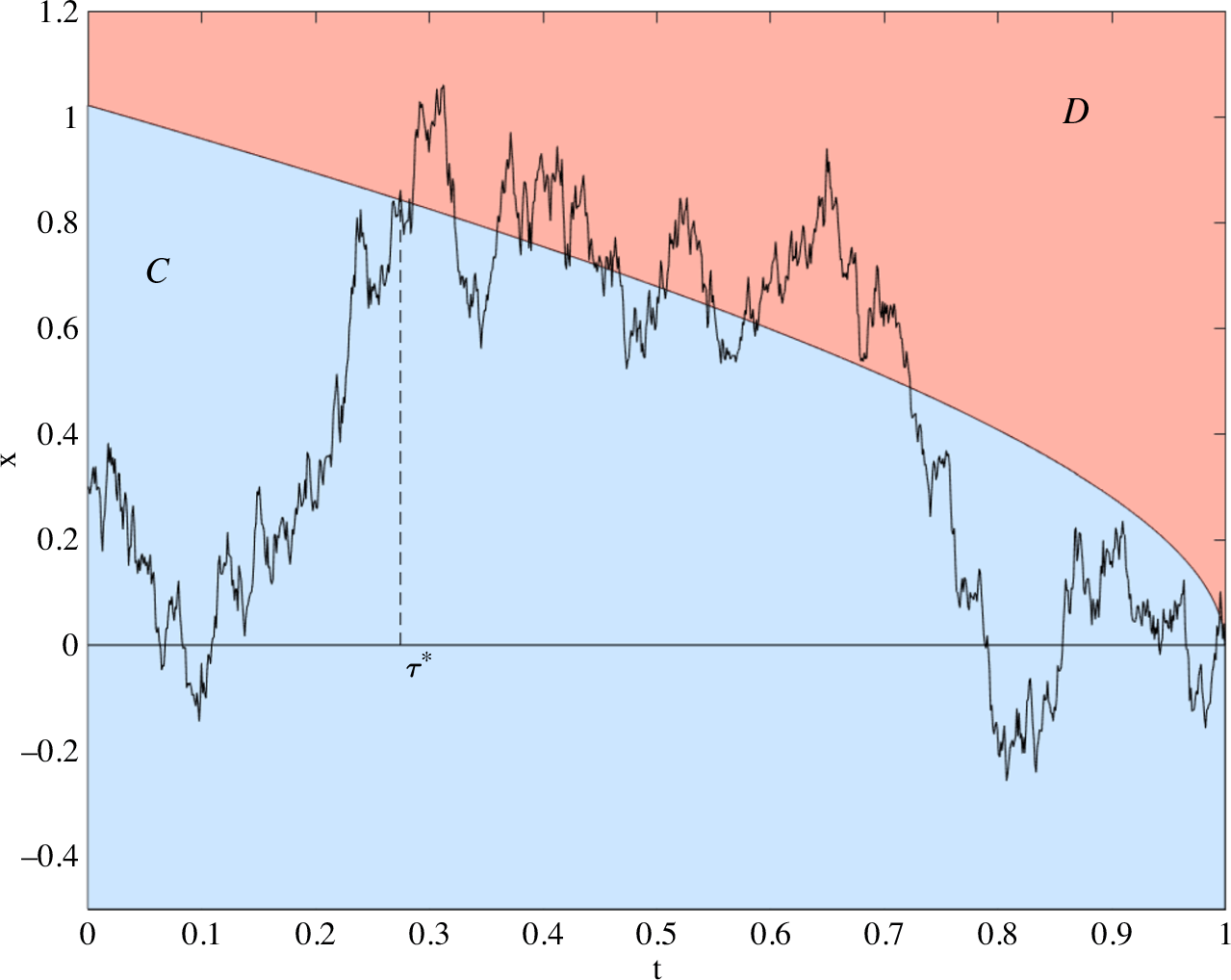
The algorithm stops when the numerical error $e_k\coloneqq \max_{j=0,\ldots,n} |b^{(k)}(t_j)-b^{(k-1)}(t_j)|$ fulfills the tolerance condition $e_k<{\varepsilon}$ , for some ${\varepsilon}>0$ . A numerical approximation of the optimal boundary is presented in Figure 1.

Figure 1:

A sample path of a Brownian bridge X starting at $X_0=0.3$ and pinned at $X_1=0$ . The Brownian bridge hits the optimal boundary at $\tau^*\approx 0.3$ . The boundary divides the state space into the continuation region ${\mathcal{C}}$ (in light blue) and the stopping region ${\mathcal{D}}$ (in red). The tolerance of the algorithm is set to ${\varepsilon}=10^{-6}$ and the equispaced time step is $h=10^{-3}$ .

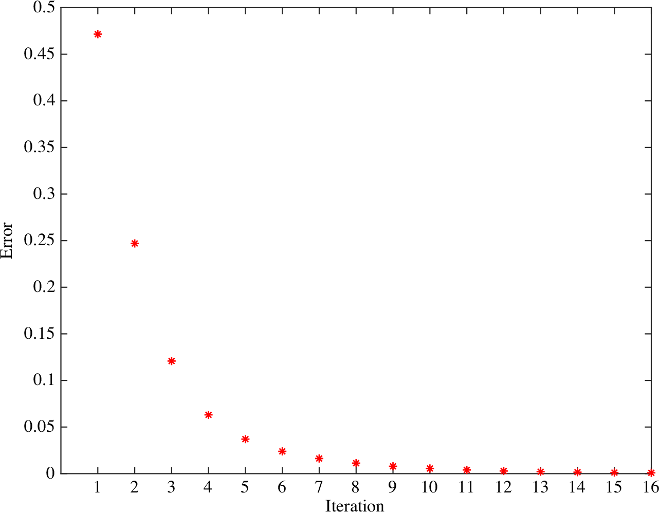
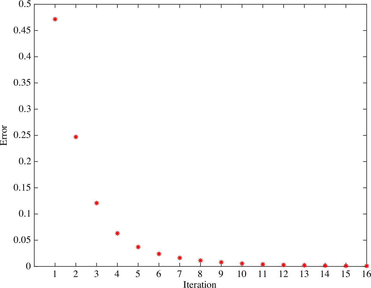
While a rigorous proof of the convergence of the scheme seems difficult and falls outside the scope of this work, in Figure 2 we show that the numerical error $e_k$ converges to zero as the number of iterations increases. Moreover, the convergence is monotone, which results in a good stability of the scheme.

Figure 2:

The trajectory of the error $e_k$ for 16 iterations of the algorithm when ${\varepsilon}=10^{-3}$ .

Figure 3:

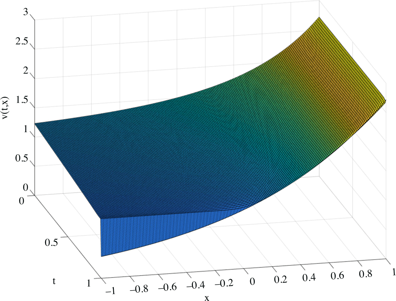
The value function surface v(t, x) plotted on a grid of points $(t,x)\in[0, 1]\times[-1,1]$ with discretisation step $h=10^{-2}$ .

Figure 4:

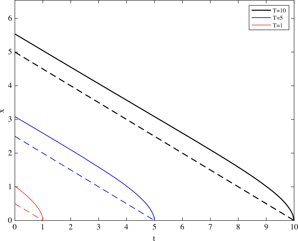
Boundary functions with starting point $t=0$ and increasing pinning times $T=1$ , $T=5$ , and $T=10$ (plotted with increasing line thickness). Notice that every boundary lies above the corresponding line $x=\tfrac{1}{2}(T-t)$ (represented by the dashed lines with the same thickness), which generalises the set ${\mathcal{Q}}$ from (25).

Finally, in Figure 3 we plot the value function as a surface in the (t, x)-plane using (45). It is interesting to observe that, as predicted by the theory, the value function exhibits a jump at $\{1\}\times(-\infty,0)$ .

Remark 3. Traditionally, integral equations as in (46) are solved by discretisation of the integral with respect to time and a backward procedure, starting from the terminal time (see, e.g., [Reference Peskir and Shiryaev23, Chapter VII, Section 27, pp. 432–433] for details in the case of the Asian option or [Reference Peskir and Shiryaev23, Chapter VIII, Section 30, p. 475] for another example; this method was developed in the seminal paper [Reference Kim19] and later extended). To the best of our knowledge, a rigorous proof of convergence for this ‘traditional’ numerical scheme is not available.

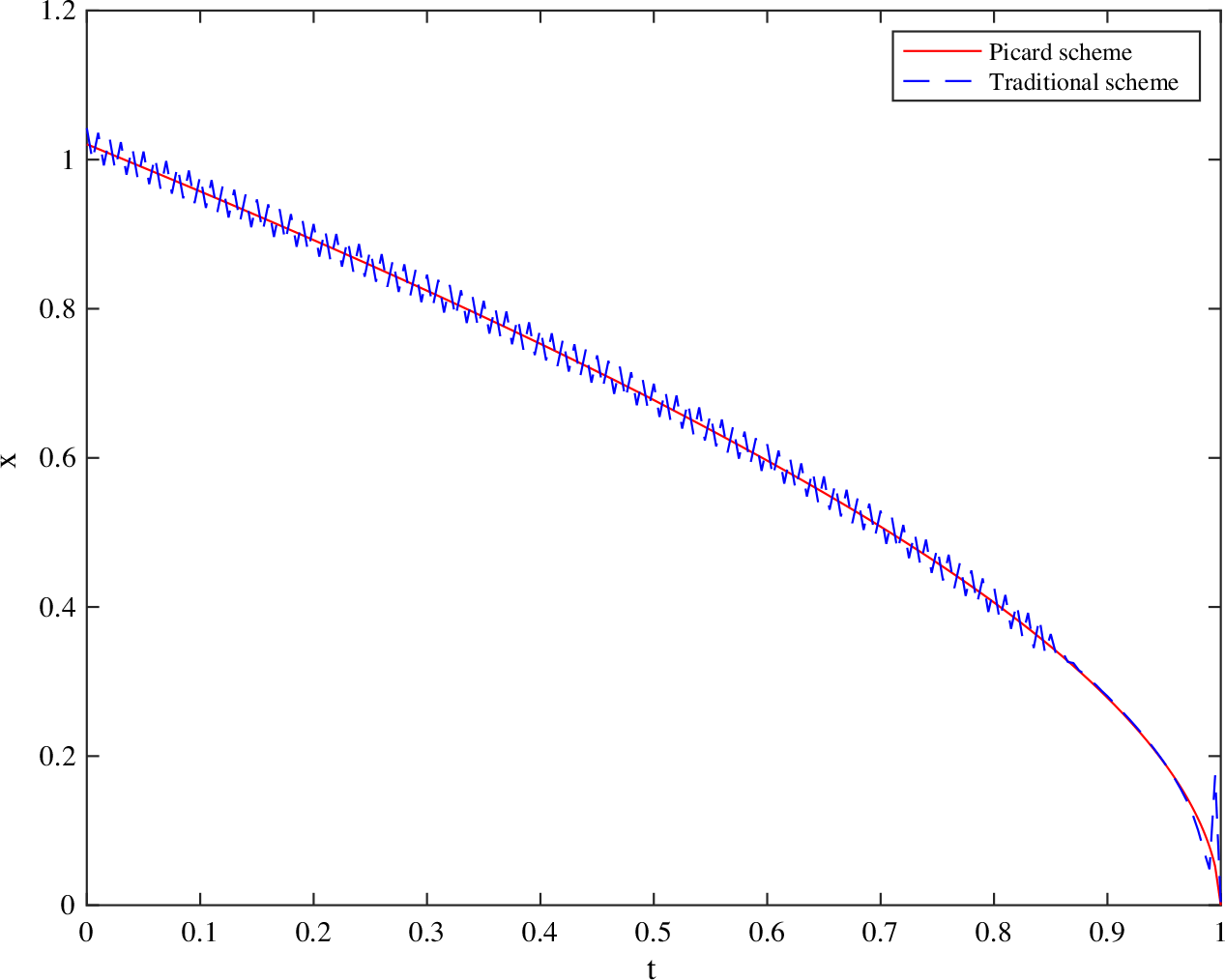
At each time step, the scheme must find the root of a highly non-linear algebraic equation, making the procedure slower than the Picard scheme that we implement, which requires no root finding (see Figure 5 for a comparison).

Figure 5:

The solution of the optimal boundary found via the Picard scheme (continuous line) and via the traditional method (dashed line). The time step is $h=5\cdot 10^{-3}$ and the tolerance is $\varepsilon=10^{-5}$ . The Picard scheme stops after 0.1 seconds and 36 iterations, the traditional method after 2.9 seconds.

Another possibility is to use finite difference methods to solve directly the free boundary problem in (18) and (19). The finite difference method, however, requires discretisation of both time and space (whereas we only discretise time), which leads to discretisation errors both in time and space and generally to a slower convergence. Moreover, in our case the coefficient associated to the first-order partial derivative $\partial_x v$ is discontinuous at $t=1$ , which causes additional difficulties.

Remark 4. After we numerically solved equation (46) and we were able to plot the boundary function as in Figure 1, we began to investigate whether a suitable fit for the boundary could be found. It is known that in the stopping problem with linear payoff $\textrm{E}[X_\tau]$ and pinning time $T=1$ , the optimal boundary can be found explicitly and it takes the form $b(t)=B\sqrt{1-t}$ (see [Reference Shepp24]). Motivated by this result we considered candidate boundaries of the form $b_T(t)=A_T(1-\exp(B_T\sqrt{T-t}))$ , where T is the pinning time of the Brownian bridge, and $A_T$ and $B_T$ are parameters to be determined.

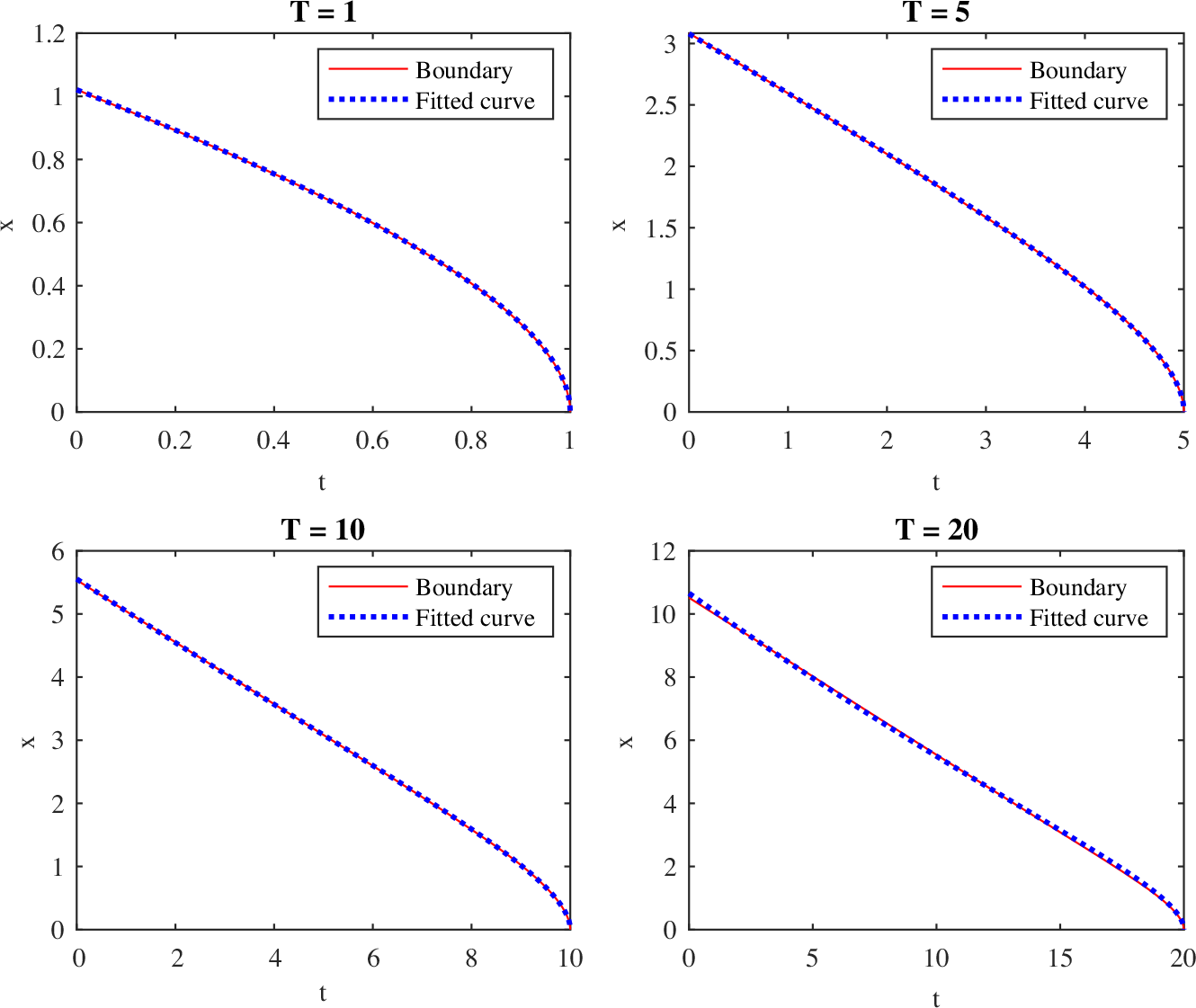
Using the ‘curve-fitting toolbox’ in Matlab to fit our ansatz to the boundaries obtained from the integral equations, we obtain an excellent fit for $T=1,5,10$ . The quality of the fit slightly deteriorates for larger T (e.g. for $T=20$ ). The results are illustrated in Figure 6. While these tests suggest that our problem might be amenable to an explicit solution, the question is more complex than in the linear payoff case (and its extensions in [Reference Ekström and Wanntorp11]) and remains open. The key difficulties are that (i) we must determine two parameters rather than one, and (ii) we do not have a good guess for the value function that would allow us to transform the free boundary problem in (18) and (19) into a solvable ordinary differential equation. Indeed, in the linear case one uses the identity in law

\[\mathsf{Law}\big(X^{t,x}_s,\, s\in[t,1]\big)=\mathsf{Law}\big(\widetilde{Z}^x_s,\,s\in[0,\infty)\big),\]

with $\widetilde{Z}^{x}_s\coloneqq (x+\sqrt{1-t}W_{s})/(1+s)$ , and obtains

\[U(t,x)\coloneqq \sup_{0\le \tau\le 1-t}\textrm{E}[X^{t,x}_{t+\tau}]=\sup_{\tau\ge 0}\textrm{E}\left[\frac{x+\sqrt{1\!-\!t}\,W_{\tau}}{1+\tau}\right]=\sqrt{1\!-\!t}\,U\left(0,\tfrac{x}{\sqrt{1-t}}\right).\]

With the exponential payoff, the same identity does not provide any useful insight.

Figure 6:

Boundary functions (continuous lines) and the corresponding fitted curves (dashed lines) of the form $b_T(t)=A_T(1-\exp(B_T\sqrt{T-t}))$ for the pinning times $T=1,5,10,20$ . The values of the parameters are, respectively, $A_1=-2.09$ , $B_1=0.4$ ; $A_5=-1.85$ , $B_5=0.43$ ; $A_{10}=-1.86$ , $B_{10}=0.44$ ; and $A_{20}=-2.27$ , $B_{20}=0.39$ .

A different approach based on finding parameters for which the guessed boundary $b_T(t)$ solves the integral equation (46) seems even harder.