1. Introduction
Compliant fins and wings have prompted long-standing interest in flexible propulsors among biologists and fluid dynamicists. Wu (Reference Wu1971a ) first predicted that flexible propulsors could provide higher efficiencies, and this was later confirmed numerically by Katz & Weihs (Reference Katz and Weihs1978). However, it is only recently that advances in materials technology have popularized flexible energy harvesters (Liu, Xiao & Cheng Reference Liu, Xiao and Cheng2013) and underwater vehicles (Low Reference Low2011), some of which can vary stiffness during operation (Park et al. Reference Park, Huh, Park and Cho2014). This newfound practicability has led to a surge in research on flexible propulsors.
The major finding of this body of work is that flexibility can boost propulsive efficiency. This finding holds true for flexible airfoils (Prempraneerach, Hover & Triantafyllou Reference Prempraneerach, Hover and Triantafyllou2003; Pederzani & Haj-Hariri Reference Pederzani and Haj-Hariri2006), and heaving and/or pitching flexible panels (Heathcote & Gursul Reference Heathcote and Gursul2007; Zhu Reference Zhu2007; Michelin & Llewellyn Reference Michelin and Llewellyn2009; Paulo, Ferreira de Sousa & Allen Reference Paulo, Ferreira de Sousa and Allen2011; Alben et al.
Reference Alben, Witt, Baker, Anderson and Lauder2012; Dewey et al.
Reference Dewey, Boschitch, Moored, Stone and Smits2013; Quinn, Lauder & Smits Reference Quinn, Lauder and Smits2014a
). When the propulsor and fluid densities have similar magnitudes, the efficiency appears to be maximized when the actuation frequency is at or near the resonant frequency of the fluid–structure system (Michelin & Llewellyn Reference Michelin and Llewellyn2009; Masoud & Alexeev Reference Masoud and Alexeev2010; Dewey et al.
Reference Dewey, Boschitch, Moored, Stone and Smits2013; Quinn et al.
Reference Quinn, Lauder and Smits2014a
). If instead the propulsor is more dense than the surrounding fluid, the inertia of the propulsor may dominate the dynamics, and fluid–structure resonance may play a lesser role; Daniel & Combes (Reference Daniel and Combes2002) and Kang et al. (Reference Kang, Aono, Cesnik and Shyy2011) provide a further discussion. In the present study, the propulsor–fluid density ratio is
 $O(1)$
, and we will show that resonance plays an important role in maximizing efficiency.
To isolate the effects of flexibility, most studies of flexible propulsors have considered either heave-only or pitch-only actuation. When considering both heave and pitch, the phase lag between the two becomes an additional input parameter. Linear theory predicts that efficiency is maximized when pitch lags heave by
 $90^{\circ }$
in the flapping cycle (Lighthill Reference Lighthill1970; Wu Reference Wu1971b
), and this has been confirmed numerically for rigid airfoils (Isogai & Shinmoto Reference Isogai and Shinmoto1999; Tuncer & Kaya Reference Tuncer and Kaya2005). In experiments, the optimal phase lag has been shown to be slightly smaller; Anderson et al. (Reference Anderson, Streitlien, Barrett and Triantafyllou1998), for example, determined
 $75^{\circ }$
to be optimal. Non-optimal values of phase lag are associated with leading-edge separation, which can lead to losses in efficiency (Wang Reference Wang2000; Lewin & Haj-Hariri Reference Lewin and Haj-Hariri2003; Kang et al.
Reference Kang, Aono, Baik, Bernal and Shyy2013).
Here, we provide the first experimental investigation of flexible panels undergoing both heave and pitch over a range of phase lags. To explore the full space of input parameters, we will use gradient-based optimization in addition to more traditional grid searches. Optimization routines have previously been used in numerical propulsor design. For example, fluid simulations have been combined with gradient-based optimization to tune the kinematics of rigid airfoils (Tuncer & Kaya Reference Tuncer and Kaya2005) and with evolutionary algorithms to tune the shape and/or kinematics of anguilliform swimmers (Kern, Koumoutsakos & Eschler Reference Kern, Koumoutsakos and Eschler2007; Tokic & Yue Reference Tokic and Yue2012; van Rees, Gazzola & Koumoutsakos Reference van Rees, Gazzola and Koumoutsakos2013). Optimization can also be applied to analytical models. Eloy & Schouveiler (Reference Eloy and Schouveiler2011), for example, used an empirical nonlinear model to tune the deformation of a two-dimensional (2D) flexible panel. Only two propulsion studies have combined optimization techniques with experimental setups. Milano & Gharib (Reference Milano and Gharib2005) used an evolutionary algorithm to maximize the lift produced by a flapping rigid plate, and Izraelevitz & Triantafyllou (Reference Izraelevitz and Triantafyllou2014) used model-based optimization to tune the in-line motion of rigid airfoils. One advantage of experimental optimization is that the analogue nature of experimental techniques is combined with the rapidity of computational optimization.
The main goal of the work presented here is to demonstrate that an experimental gradient-based optimization routine can be used to maximize the efficiency of flexible propulsors. We will show that optimization is especially well-suited for flexible propulsors, where achieving resonance requires particular combinations of input parameters that are unknown a priori. In addition to the optimization, we will investigate the causes of the maximal efficiencies by considering select subspaces of the input parameters and conducting particle image velocimetry (PIV) on a sample of near-optimal cases. We will demonstrate that the efficiency is globally maximized when: (i) the Strouhal number is within an optimal range that varies weakly with amplitude and boundary conditions; (ii) the panel is actuated at a resonant frequency of the fluid–panel system; (iii) heave amplitude is tuned such that trailing-edge amplitude is maximized while flow along the body remains attached; and (iv) the maximum pitch angle and phase lag are chosen so that the effective angle of attack is minimized.
2. Experimental methods
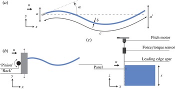
Experiments were conducted on a flexible rectangular panel suspended in a recirculating water channel with flow speed
 $u$
. The chord
 $c$
, span
 $s$
, and thickness
 ${\it\delta}$
of the panel were 195 mm, 150 mm, and 0.11 mm, respectively. The panel had an elastic modulus
 $E=3.8$
GPa, resulting in a bending stiffness
 $b=6.9\times 10^{-5}$
 $\text{N}~\text{m}^{2}$
, where
 $b\equiv Es{\it\delta}^{3}/(12(1-{\it\nu}^{2}))$
, and Poisson’s ratio
 ${\it\nu}$
was estimated to be 0.3. The elastic modulus was measured by tensile tests of the polyethylene from which the panel was made. A deflection test was also used to measure the bending stiffness of the panel, and the resulting estimate agreed with the tensile tests to within 10 %.
The panel was actuated at the leading edge by an aluminium spar (chord = 10 mm, thickness = 3 mm) undergoing heave and pitch oscillations. The oscillations were such that the lateral position
 $h$
and angle of attack
 ${\it\alpha}$
of the spar followed
 $h=a\;\text{sin}(2{\rm\pi}\,f\,t)$
and
 ${\it\alpha}={\it\alpha}_{0}\;\text{sin}(2{\rm\pi}\,f\,t-{\it\phi})$
, where
 $a$
is the heave amplitude,
 ${\it\alpha}_{0}$
is the maximum pitch angle,
 $f$
is the frequency of oscillation,
 $t$
is time, and
 ${\it\phi}$
is the phase lag between heave and pitch. The remainder of the panel deformed passively, finishing with a trailing-edge amplitude
 $a^{\prime }$
. The motions were produced by connecting the spar to a pitch motor (Pittman, GM8724S009) seated beneath a rack that heaved back and forth under the action of a second motor (MCG, IB23007) (see figure 1).
Experimental arrangement. (a) Length scale definitions; (b) top view; (c) side view.

A six-axis force–torque sensor (ATI Inc., Nano-17 SI-50-0.5) was used to measure streamwise forces
 $\mathscr{F}_{x}$
, lateral forces
 $\mathscr{F}_{y}$
, and
 $z$
-torques
 $\mathscr{Q}_{z}$
. The true lateral
 ${\dot{h}}$
and angular
 $\dot{{\it\alpha}}$
velocities of the spar were recorded using two rotary encoders. Together, these force and velocity data give the power input to the fluid
 ${\wp}$
according to
 ${\wp}=-\mathscr{F}_{y}{\dot{h}}-\mathscr{Q}_{z}\dot{{\it\alpha}}$
. Time-averages were obtained by averaging over the largest number of oscillation cycles possible in a 10 s period of data acquisition. We will use ‘net thrust’
 $\bar{{\it\tau}}$
and ‘net power’
 $\bar{{\wp}}$
to refer to time-averaged streamwise force and power input to the fluid, respectively. Of particular importance to swimming performance is the propulsive efficiency
 ${\it\eta}\equiv \bar{{\it\tau}}u/\bar{{\wp}}$
. The average variance between trials for net thrust and power was
 $\pm 5$
mN and
 $\pm 1$
mW, resulting in
 $3\,\%$
uncertainty in the efficiency.
The chosen propulsive efficiency metric, often called the Froude efficiency, represents the fraction of energy transferred to the wake resulting in positive thrust. This metric is only defined when the thrust produced by the propulsor exceeds the drag incurred by the flow. Fully autonomous swimmers require that their net thrust be zero for steady swimming, and in this case the more appropriate metric is the cost of transport,
 $u/\bar{{\wp}}$
. Our treatment of efficiency is therefore best-suited for propulsors that operate with net thrust in order to drive drag-producing payloads. Given the
 $O(1)$
aspect ratio of our panel, our results may apply most directly to swimmers with broad flattened fins, such as rays and skates or batoid-inspired vehicles.
The oscillations of the leading-edge spar define four of the five input parameters to the system (
 $f,{\it\phi},a$
, and
 ${\it\alpha}_{0}$
), with the fifth input being the flow speed of the water channel (
 $u$
). The time to conduct full sweeps of the parameter space
 $t_{\mathit{exp}}$
depends exponentially on the number of input parameters
 $n$
, that is,
 $t_{\mathit{exp}}\propto \text{e}^{n}$
. Including multiple trials and resetting time, the proportionality constant for the current setup is approximately 1 h. This limitation precludes any full sweeps of the full five-dimensional (5D) parameter space. Instead, we will consider selected subspaces of the parameter space and employ gradient-based optimization to seek the global maxima of the full space.
The largest subspace we considered spans the space of heave-only motions (
 ${\it\alpha}_{0}=0$
). Data were taken via grid search over 23 frequencies ranging from 0.6 to 2.8 Hz, 14 flow speeds ranging from 25 to
 $360~\text{mm}~\text{s}^{-1}$
, and four amplitudes ranging from 6 to 18 mm. This subspace was chosen to overlap with previous heave-only studies (Quinn et al.
Reference Quinn, Lauder and Smits2014a
) and to demonstrate some general features of the efficiency manifold. The subspace covers Strouhal numbers and Reynolds numbers that are typical of fishes and bio-inspired propulsors with similar chord lengths to our panel (Lauder, Flammang & Alben Reference Lauder, Flammang and Alben2012; Shelton, Thornycroft & Lauder Reference Shelton, Thornycroft and Lauder2014). Two smaller subspaces were chosen to isolate the effects of pitch and phase offset. These subspaces correspond to conditions near the two optima discovered by the gradient-based optimization scheme. Here, the heave amplitude, frequency, and flow speed were fixed at their optimum values, while maximum pitch angle and phase offset were kept variable. Data were taken at 11 maximum pitch angles ranging from
 $0^{\circ }$
to
 $30^{\circ }$
and 16 phase offsets ranging from
 $0^{\circ }$
to
 $337.5^{\circ }$
. The upper bound for maximum pitch angle was a limitation based on load constraints of the force sensor.
Some optimization studies have used advanced learning algorithms (e.g. SNOPT by Gill, Murray & Saunders Reference Gill, Murray and Saunders2005 was used by Izraelevitz & Triantafyllou Reference Izraelevitz and Triantafyllou2014), but we chose an archetypal gradient-based algorithm in order to demonstrate the robustness of the technique. The algorithm is a form of iterated local search based on classical learning algorithms from Snyman (Reference Snyman2005). During each iteration, the inputs are shifted in the direction of the estimated gradient of the efficiency manifold, and the cycle is repeated until a minimum step size is reached. Further details of the method are given in appendix A.
At several sample conditions, PIV was conducted at the midspan. The laser sheet was generated by a continuous 10 W argon-ion laser (Coherent, Innova 70-C), and the particles were hollow silver-coated glass beads with an average diameter of
 $12~{\rm\mu}\text{m}$
. Images were taken at 250 Hz with
 $1024\times 1024$
resolution (Photron, FASTCAM 1024 PCI). The velocity field was calculated using Davis 8.1.3, the spatial cross-correlation algorithm developed by LaVision Inc. (Stanislas et al.
Reference Stanislas, Okamoto, Kahler and Westerweel2005). Four passes with 50 % overlap were conducted on the data: two with
 $64\times 64$
pixel windows and two with
 $24\times 24$
. The resulting velocity field consisted of
 $86\times 86$
vectors. Phase-averaged velocity fields were calculated using the same number of cycles as the time-averaged force data. The PIV images were also used to calculate trailing-edge amplitude, which was taken to be the average difference between extrema of the trailing-edge position.
As a control case, a rigid NACA 0012 airfoil (67 mm chord) was run through the same testing procedure at sample conditions, chosen to overlap with those used for the flexible panel and with a previous NACA 0012 dataset taken in the same water channel (Lauder et al.
Reference Lauder, Lim, Shelton, Witt, Anderson and Tangorra2011). For these cases, the heave amplitude, maximum pitch angle, and phase offset were fixed at 13 mm,
 $10^{\circ }$
, and
 $90^{\circ }$
, respectively. Data were taken at 11 frequencies ranging from 1.1 to 2.1 Hz and 11 flow speeds ranging from 30 to
 $180~\text{mm}~\text{s}^{-1}$
.
3. Scaling considerations
The five input parameters to the system are the flow speed
 $u$
, oscillation frequency
 $f$
, heave amplitude
 $a$
, maximum pitch angle
 ${\it\alpha}_{0}$
, and heave–pitch phase lag
 ${\it\phi}$
. In cases where PIV was conducted, the trailing-edge amplitude
 $a^{\prime }$
is also known. Additional constants are the density
 ${\it\rho}$
and viscosity
 ${\it\mu}$
of the water, and the chord
 $c$
, span
 $s$
, and bending stiffness
 $b$
of the propulsor. These 11 variables produce eight dimensionless parameters. One of them, the aspect ratio
 $AR\equiv s/c$
, is fixed for this experiment at 0.77. Another, the Reynolds number based on the chord,
 $Re_{c}\equiv {\it\rho}uc/{\it\mu}$
, ranges from 5000 to 70 000 in this study, and at these large Reynolds numbers pressure forces are assumed to dominate over viscous forces so that
 $Re_{c}$
will not be considered further. The dimensionless trailing-edge amplitude
 $a^{\prime }/a$
is an output of the system and will be used to verify the location of resonant frequencies.
The remaining five dimensionless parameters provide an alternative description of the five-dimensional input space over which we will optimize efficiency. First we have
 ${\it\alpha}_{0}$
and
 ${\it\phi}$
, which are already dimensionless. Next we have the amplitude–chord ratio
 $a^{\ast }\equiv a/c$
and the Strouhal number
 $St\equiv 2af/u$
(
 $a$
is used as a proxy for the width of the wake since it is prescribed). The final parameter must incorporate the bending stiffness of the panel. By introducing an added-mass term into linear beam theory, it can be estimated that the first eigenfrequency of the fluid–panel system
 $\hat{f}_{1}$
is
 $(b/(\mathscr{M}{\it\rho}sc^{5}))^{1/2}$
, where
 $\mathscr{M}$
is a constant (see appendix B). We are thus motivated to introduce a second dimensionless frequency based on this time scale, the ‘flexural frequency’
 $f^{\ast }\equiv f/\hat{f}_{1}$
, where
 $\mathscr{M}$
will be set to 1 for now (its actual value will be discussed later). Whereas
 $St$
compares the actuation frequency to time scales of the incoming flow,
 $f^{\ast }$
relates the actuation frequency to time scales of fluid–structure resonance.
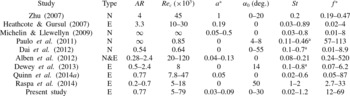
Table 1 compares the range of dimensionless input parameters for several studies of propulsive flexible panels. Note that
 ${\it\phi}$
has been omitted because most studies examine heave or pitch only. The exceptions are Zhu (Reference Zhu2007), where
 ${\it\phi}$
was fixed at
 $90^{\circ }$
, and this study, where
 ${\it\phi}$
ranges from
 $0^{\circ }$
to
 $360^{\circ }$
. We will focus on low heave amplitudes and high flexibilities (high values of
 $f^{\ast }$
) because this configuration can excite multiple resonant modes at modest frequencies (
 $f\;(\text{Hz})=O(1)$
).
Dimensionless parameters used in recent flexible panel studies. Type
 $\equiv$
N (numerical) or E (experimental); aspect ratio
 $AR\equiv s/c$
; Reynolds number
 $Re_{c}\equiv {\it\rho}uc/{\rm\mu}$
; amplitude–chord ratio
 $a^{\ast }\equiv a/c$
; maximum pitch angle
 ${\it\alpha}_{0}$
; Strouhal number
 $St\equiv 2a\,f/u$
; flexural frequency
 $f^{\ast }\equiv f/\hat{f}_{1}$
.
 $^{\text{a}}$
Designates
 $St$
values that used a direct measurement of
 $a^{\prime }$
in place of
 $a$
.

4. Propulsive efficiency results
Before introducing flexibility, we first consider the rigid airfoil control case. Scaling arguments based on added mass (e.g. Dewey et al.
Reference Dewey, Boschitch, Moored, Stone and Smits2013 and Quinn et al.
Reference Quinn, Moored, Dewey and Smits2014b
) suggest that for low-amplitude rigid airfoils swimming at high Reynolds numbers and moderate Strouhal numbers, the time-averaged net thrust
 $\bar{{\it\tau}}$
and power
 $\bar{{\wp}}$
scale according to
 $$\begin{eqnarray}\bar{{\it\tau}}\sim {\it\rho}sc\,f^{2}a^{2};\quad \bar{{\wp}}\sim {\it\rho}sc\,f^{2}a^{2}u.\end{eqnarray}$$
These scalings demonstrate why
 ${\it\eta}$
(
 $\equiv \bar{{\it\tau}}u/\bar{{\wp}}$
) is
 $O(1)$
under typical swimming conditions, but to explain the variation in the efficiency
 ${\it\eta}$
, one must turn to potential flow models that include a wake. Such models reveal that efficiency tapers off with increasing
 $St$
and drops off sharply when
 $St\ll 1$
(Lighthill Reference Lighthill1975). In a real flow, viscous drag also causes
 ${\it\eta}$
to become negative below some threshold Strouhal number. In practice, these trends cause a local maximum in efficiency to occur at
 $St\approx 0.2{-}0.4$
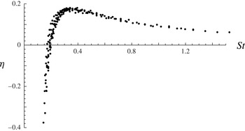
for typical swimmers (Taylor, Nudds & Thomas Reference Taylor, Nudds and Thomas2003), although the range may be wider (Eloy Reference Eloy2012). These tendencies have been observed in a variety of experimental and numerical studies (see e.g. Triantafyllou, Triantafyllou & Yue (Reference Triantafyllou, Triantafyllou and Yue2000) for a review), and were reproduced as means of a control case for the present study (see figure 2).
Propulsive efficiency as a function of Strouhal number for a pitching and heaving rigid NACA0012 airfoil.
 $a^{\ast }=0.19$
,
 ${\it\phi}=90^{\circ }$
.

4.1. Heave-only motions
We now compare the rigid case with the subspace of heave-only motions (
 ${\it\alpha}_{0}=0$
) for our flexible propulsor. With the additional time scale provided by flexibility, both
 $St$
and
 $f^{\ast }$
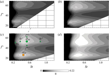
play a role in determining efficiency. This effect is illustrated in figure 3 by contour plots of efficiency over a variety of
 $St$
and
 $f^{\ast }$
values. Moving from low to high
 $St$
at a fixed value of
 $f^{\ast }$
shows the same sharp rise and slow taper observed in figure 2. Varying
 $f^{\ast }$
, however, reveals a multimodal response in efficiency as the fluid–panel system passes through resonant modes. The peaks are known to correspond to resonance because the same propulsor was previously shown to exhibit local maxima in trailing-edge amplitude at these particular frequencies (Quinn et al.
Reference Quinn, Lauder and Smits2014a
). The global maxima in efficiency occur when the optimum Strouhal number aligns with fluid–structure resonance.
Contour plots of propulsive efficiency for heave-only motions: (a)
 $a^{\ast }=0.03$
; (b)
 $a^{\ast }=0.05$
; (c)
 $a^{\ast }=0.07$
; (d)
 $a^{\ast }=0.09$
. Labelled circles show conditions at which PIV was conducted (see § 5).

The efficiency also increases with amplitude, presumably because the relative contribution of viscous drag decreases. Alternatively, the same effect can be explained with actuator disc theory (Anderson et al.
Reference Anderson, Streitlien, Barrett and Triantafyllou1998). High amplitudes must lead to a loss of efficiency, but no such effect was observed for the small amplitudes studied here. The global optimum over all heave-only conditions was found to be
 ${\it\eta}=0.23$
at
 $St=0.53$
,
 $f^{\ast }=57$
, and
 $a^{\ast }=0.09$
. However, within experimental error, this condition was equally efficient as the peak in the other mode where
 ${\it\eta}=0.21$
at
 $St=0.40$
,
 $f^{\ast }=27$
, and
 $a^{\ast }=0.09$
. We will refer to these two heave-only optima as
 $\mathscr{A}_{\mathit{3D}}$
and
 $\mathscr{B}_{\mathit{3D}}$
to signify that the optimization took place over three dimensions. The ratio between optimum
 $f^{\ast }$
values (
 $=57/27=2.11$
) is strikingly similar to the predictions of linear beam theory (see appendix B), strongly suggesting that for our propulsive system added mass plays the most important role in scaling the fluid–structure resonance.
The heave-only power data did not show the
 $u$
-dependence expected from (4.1), presumably because those predictions are based on prescribed kinematics, whereas our propulsor deforms passively. To try to resolve this issue, we replace
 $u$
with
 $c\,\hat{f}_{1}$
, a velocity based on the fundamental frequency. Guaranteeing the appropriateness of this particular replacement would require a separate study of panels with varying size and stiffness, but the replacement is chosen here because it uses the only remaining time scale in the problem. The modified scaling predictions can then be written in dimensionless form as
 $$\begin{eqnarray}\bar{{\it\tau}}^{\ast }\sim \bar{{\wp}}^{\ast }\sim (f^{\ast }a^{\ast })^{2},\end{eqnarray}$$
where thrust and power have been non-dimensionalized using the bending stiffness
 $b$
and the first-harmonic frequency
 $\hat{f}_{1}$
, that is,
 $$\begin{eqnarray}\bar{{\it\tau}}^{\ast }\equiv \frac{\bar{{\it\tau}}}{b/c^{2}},\quad \bar{{\wp}}^{\ast }\equiv \frac{\bar{{\wp}}}{b\hat{f}_{1}/c}.\end{eqnarray}$$
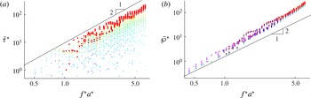
For heave-only motions, figure 4 demonstrates that the proposed scaling gives the right trend for the power over a wide range of frequencies and amplitudes. The thrust, however, increases more slowly than predicted by the trend at low Strouhal numbers. At higher Strouhal numbers, added-mass forces dominate over viscous forces, and thrust approaches the slope predicted by the scaling. The bumps on the line to which thrust is converging are evidence of resonances, which lead to the local maxima in efficiency (figure 3). The power shows a better collapse than thrust because it scales with lateral forces at the leading edge, which are an order of magnitude higher than the viscous drag. Together, figures 3 and 4 demonstrate that efficiency is multimodal because of its sensitivity to slight changes in thrust at resonance, but that net thrust and power still scale predictably in the larger scope of the parameter space.
Dimensionless performance coefficients for heave-only motions. Log–log scale. (a) Dimensionless net thrust (
 $\bar{{\it\tau}}^{\ast }$
); (b) dimensionless net power (
 $\bar{{\wp}}^{\ast }$
). Bold circles correspond to conditions where
 $St\geqslant 0.6$
.

4.2. Combined heave and pitch motions
We now consider leading-edge motions that include pitch, that is, where
 ${\it\alpha}_{0}\neq 0$
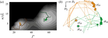
. To begin, the gradient-based optimization scheme was used to find the maximum efficiency conditions. Figure 5(a) shows the algorithm validated in two dimensions for the heave-only case. Note that
 $u/(c\,\hat{f}_{1})$
was used in place of
 $St$
for the optimization – this substitution was chosen to decrease the runtime of the algorithm by limiting changes in flow speed between steps. The substitution does not affect the dimensionality of the parameter space, and we will convert back to
 $St$
values in subsequent analyses. Figure 5(b) shows a 2D projection of the trajectories through the 5D state space as the algorithm converges on optimum conditions. The particular projection was chosen using multi-dimensional scaling (MDS). In this technique, the
 ${\it\Pi}_{1}{-}{\it\Pi}_{2}$
plane is chosen such that the L2 norm in the plane is most similar to the L2 norm in the 5D parameter space. In this way, distances in the
 ${\it\Pi}_{1}{-}{\it\Pi}_{2}$
plane are representative of distances in state space (see e.g. Borg & Groenen (Reference Borg and Groenen2005) for a full description of MDS).
The MDS projection illustrates that the optimization converges on two clusters in state space, and we will refer to the averaged conditions of these clusters as
 $\mathscr{A}_{\mathit{5D}}$
and
 $\mathscr{B}_{\mathit{5D}}$
. Table 2 shows the conditions at each optimum, as well as the conditions at the heave-only optima for comparison. The fact that the
 $f^{\ast }$
values are relatively unchanged is evidence that these newly discovered optima are the same resonant modes as those observed in the heave-only case. This observation is consistent with linear beam theory in that the boundary conditions for the perturbation component of the solution have not changed (one end clamped, one end free), and so the eigenfrequencies should be the same in both cases. The major changes between the two cases are: (i) the heave-only optima have higher
 $St$
values, meaning the heave-only propulsors need to heave faster to achieve the same zero net thrust flow speed; (ii) an equilibrium amplitude was reached in the trials with pitch (
 $a^{\ast }=0.07$
), suggesting that dynamic stall was a limiting factor in the 5D optimization; and (iii) introducing pitch nearly doubles the propulsive efficiencies. The errors reported are the standard deviations in the clusters of optimal design variables to which the procedure converged. These errors characterize the reproducibility of the procedure and the sensitivity to initial conditions.
(a) Four gradient-based optimization routines demonstrated on a 2D subset of the parameter space.
 $a^{\ast }=0.05$
. Trajectories are superimposed on a contour plot of propulsive efficiency. Efficiency scaling as in figure 3. (b) A 2D projection of the 5D trajectories chosen by 15 gradient-based optimization routines; the
 ${\it\Pi}_{1}{-}{\it\Pi}_{2}$
plane was chosen via multi-dimensional scaling. Outlined circles denote the endpoints of the trajectories. The two double-outlined circles show projections of the heave-only optima (
 $\mathscr{A}_{\mathit{3D}}$
and
 $\mathscr{B}_{\mathit{3D}}$
) for reference.

Input parameters and efficiencies at optimum conditions for heave-only motions (
 $\mathscr{A}_{\mathit{3D}}$
and
 $\mathscr{B}_{\mathit{3D}}$
) and heave/pitch motions (
 $\mathscr{A}_{\mathit{5D}}$
and
 $\mathscr{B}_{\mathit{5D}}$
).

To explore the effects of phase offset, we consider two projections onto the
 ${\it\phi}{-}{\it\alpha}_{0}$
plane in the vicinity of
 $\mathscr{A}_{\mathit{5D}}$
and
 $\mathscr{B}_{\mathit{5D}}$
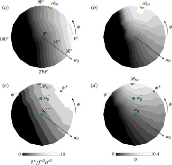
. Figure 6 shows the projections for net thrust and efficiency, and it demonstrates that introducing pitch is not always advantageous. For some values of
 ${\it\phi}$
, introducing pitch can decrease thrust and efficiency, and can even push the propulsor into a drag-producing regime.
An important parameter when interpreting these plots is the effective angle of attack of the leading edge,
 $$\begin{eqnarray}{\it\alpha}_{\mathit{eff}}={\it\alpha}+\text{arctan}\frac{{\dot{h}}}{u},\end{eqnarray}$$
which includes the geometric angle of attack and the relative angle of attack caused by motion perpendicular to the incoming flow. The effective angle of attack is minimized when
 ${\it\phi}=90^{\circ }$
and maximized when
 ${\it\phi}=270^{\circ }$
, and in general lower values have been associated with higher efficiencies (Kang et al.
Reference Kang, Aono, Baik, Bernal and Shyy2013). The trailing-edge amplitude, however, is maximized near
 ${\it\phi}=0^{\circ }$
and minimized near
 ${\it\phi}=180^{\circ }$
, and the higher trailing-edge amplitudes at low values of
 ${\it\phi}$
can increase thrust and therefore shift the phase for optimum efficiency to values less than
 $90^{\circ }$
. This effect has been observed for rigid airfoils (Anderson et al.
Reference Anderson, Streitlien, Barrett and Triantafyllou1998) and is consistent with the thrusts and efficiencies found near
 $\mathscr{A}_{\mathit{5D}}$
(figure 6
a,b). The phase at
 $\mathscr{B}_{\mathit{5D}}$
, however, is indistinguishable from
 $90^{\circ }$
within the experimental error. Conditions near
 $\mathscr{B}_{\mathit{5D}}$
have higher
 ${\it\alpha}_{\mathit{eff}}$
values than those near
 $\mathscr{A}_{\mathit{5D}}$
, and it appears that this feature makes minimizing
 ${\it\alpha}_{\mathit{eff}}$
more important than maximizing trailing-edge amplitude near
 $\mathscr{B}_{\mathit{5D}}$
.
Contour plots of dimensionless net thrust and efficiency in the
 ${\it\alpha}_{0}{-}{\it\phi}$
plane: (a) net thrust near
 $\mathscr{A}_{\mathit{5D}}$
; (b) efficiency near
 $\mathscr{A}_{\mathit{5D}}$
; (c) net thrust near
 $\mathscr{B}_{\mathit{5D}}$
; (d) efficiency near
 $\mathscr{B}_{\mathit{5D}}$
. Labelled circles show conditions at which PIV was conducted (see § 5).

5. Flow field results
To investigate the origins of the efficiency maxima, we turn to PIV images of the flow surrounding the panel. All of the images shown are phase-averaged snapshots of vorticity at the moment when the leading edge passes the
 $y$
-axis headed toward negative
 $y$
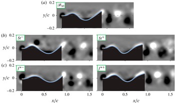
-values since this point best distinguishes the various cases. Figure 7 shows the flow field for optimum conditions
 $\mathscr{A}_{\mathit{3D}}$
and
 $\mathscr{A}_{\mathit{5D}}$
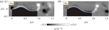
. Both flows are characterized by a thin layer of vorticity along the panel and a 2S reverse von Kármán street in the wake. The efficiency measurements, however, showed that
 $\mathscr{A}_{\mathit{5D}}$
demonstrates nearly double the efficiency of
 $\mathscr{A}_{\mathit{3D}}$
. A primary difference between the two cases is the presence of a leading-edge vortex in
 $\mathscr{A}_{\mathit{3D}}$
(figure 7
a). It appears that by decreasing the effective angle of attack, the non-zero pitch angle reduces leading-edge separation. Introducing pitch also leads to a lower Strouhal number at optimum conditions (
 $St=0.26$
compared to 0.40), which is known to be in the range of Strouhal numbers that optimize wake stability (Triantafyllou, Triantafyllou & Grosenbaugh Reference Triantafyllou, Triantafyllou and Grosenbaugh1993). This feature is reflected by the greater coherence of the vortex street for
 $\mathscr{A}_{\mathit{5D}}$
(figure 7
b).
Phase-averaged density plots of vorticity: (a) first optimum condition in the heave-only subspace (
 $\mathscr{A}_{\mathit{3D}}$
),
 $St=0.40$
,
 $f^{\ast }=27.0$
,
 $a^{\ast }=0.09$
; (b) optimum condition in the full parameter space (
 $\mathscr{A}_{\mathit{5D}}$
),
 $St=0.26$
,
 $f^{\ast }=24.8$
,
 $a^{\ast }=0.07$
,
 ${\it\alpha}=30^{\circ }$
,
 ${\it\phi}=76^{\circ }$
. Labels correspond to labelled circles in figures 3 and 6.

To examine the effect of Strouhal number more closely, we consider perturbations from an optimum condition, this time from
 $\mathscr{B}_{\mathit{3D}}$
. Figure 8 shows the flow field at
 $\mathscr{B}_{\mathit{3D}}$
as well as at non-optimal values of
 $St$
and
 $f^{\ast }$
. Strouhal numbers less than and greater than optimal will be referred to as
 $St^{-}$
and
 $St^{+}$
, respectively, and other parameters will follow the same convention. When
 $St$
is lower than optimal (
 $St^{-}$
, figure 8
b), the wave along the body is too slow to keep pace with the incoming flow, and a large vortex detaches from the body just downstream of the first peak in lateral position. At
 $St^{+}$
, no separation occurs along the body, but the vortices in the wake break down farther upstream. The thrust and power data confirm that these conditions are associated with lower efficiencies.
Phase-averaged density plots of vorticity: (a) second optimum condition in the heave-only subspace (
 $\mathscr{B}_{\mathit{3D}}$
),
 $St=0.53$
,
 $f^{\ast }=56.8$
,
 $a^{\ast }=0.09$
; (b) non-optimum
 $St$
conditions near
 $\mathscr{B}_{\mathit{3D}}$
,
 $St=0.39$
for
 $St^{-}$
and
 $St=0.86$
for
 $St^{+}$
; (c) non-optimum
 $f^{\ast }$
conditions near
 $\mathscr{B}_{\mathit{3D}}$
,
 $f^{\ast }=44.6$
for
 ${f^{\ast }}^{-}$
and
 $f^{\ast }=61.9$
for
 ${f^{\ast }}^{+}$
. All other variables were held at their optimum values. Labels correspond to labelled circles in figure 3. Vorticity scaling as in figure 7.

Variations in
 $f^{\ast }$
lead to less significant differences in the flow field, as seen in figure 8(c). The
 ${f^{\ast }}^{-}$
case shows the beginnings of a transition to a 2P wake, though this may be due more to the lower flow speed required to keep
 $St$
constant when decreasing
 $f^{\ast }$
. The more significant difference is believed to be the lower trailing-edge amplitudes observed at non-optimal
 $f^{\ast }$
values. Compared with
 $a^{\prime }/a=1.68$
at
 $\mathscr{B}_{\mathit{3D}}$
, the low and high
 $f^{\ast }$
conditions give
 $a^{\prime }/a=1.66$
and 1.52, respectively. At the same
 $f^{\ast }$
values but with the flow speed fixed at its respective optimal value, the decreases were more pronounced, with
 $a^{\prime }/a=1.63$
and 1.51. An error analysis of the edge tracking technique suggests that
 $\pm 0.02$
is a proper confidence interval for
 $a^{\prime }/a$
, so these decreases are significant. The zero in
 $\partial a^{\prime }/\partial f^{\ast }$
at optimal conditions confirms that
 $f^{\ast }$
is associated with resonance, and that the efficiency is locally maximized at resonant frequencies of the fluid–structure system.
Since the efficiency increases with
 $a^{\ast }$
through the full space of
 $a^{\ast }$
values (
 $0.03{-}0.09$
), it may be more revealing to consider the effects of varying
 $a^{\ast }$
around
 $\mathscr{B}_{\mathit{5D}}$
, where the optimum
 $a^{\ast }$
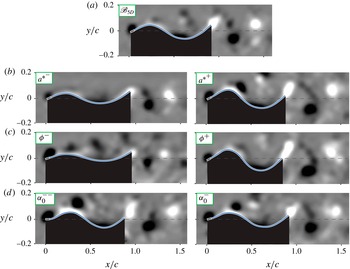
value was 0.07. Figure 9 shows the flow field at non-optimal values of
 $a^{\ast }$
, as well as at non-optimal values of
 ${\it\phi}$
and
 ${\it\alpha}$
. For the
 $a^{\ast }$
perturbations, flow speed was kept constant instead of
 $St$
, because higher flow speeds reduce the amplitude along the body and interfere with conclusions about amplitude effects. In the case of
 ${a^{\ast }}^{+}$
, amplitudes higher than optimal lead to detached flow along the body. Presumably the lateral pressure gradients become sufficiently adverse for the boundary layer to separate from the panel. The
 ${a^{\ast }}^{-}$
case shows no such separation, while the optimal case shows the beginnings of separation. The efficiency data indicated that in this low-amplitude regime, higher amplitudes are associated with higher efficiencies. It appears, therefore, that the efficiency is optimized when the amplitude is as high as possible but low enough for the flow to stay attached along the body.
Phase-averaged density plots of vorticity: (a) second optimum in the full parameter space (
 $\mathscr{B}_{\mathit{5D}}$
),
 $St=0.33$
,
 $f^{\ast }=50.8$
,
 $a^{\ast }=0.07$
,
 ${\it\alpha}=30^{\circ }$
,
 ${\it\phi}=96^{\circ }$
; (b) non-optimum
 $a^{\ast }$
conditions near
 $\mathscr{B}_{\mathit{5D}}$
,
 $a^{\ast }=0.05$
for
 ${a^{\ast }}^{-}$
and
 $a^{\ast }=0.09$
for
 ${a^{\ast }}^{+}$
; (c) non-optimum
 ${\it\phi}$
conditions near
 $\mathscr{B}_{\mathit{5D}}$
,
 ${\it\phi}=41^{\circ }$
for
 ${\it\phi}^{-}$
and
 ${\it\phi}=141^{\circ }$
for
 ${\it\phi}^{+}$
; (d) non-optimum
 ${\it\alpha}$
conditions near
 $\mathscr{B}_{\mathit{5D}}$
,
 ${\it\alpha}=15^{\circ }$
for
 ${\it\alpha}^{-}$
and
 ${\it\alpha}=0^{\circ }$
for
 ${\it\alpha}^{--}$
. Labels correspond to labelled circles in figure 6. Vorticity scaling as in figure 7.

Changing
 ${\it\phi}$
has severe consequences for the surrounding flow field (figure 9
c). In the
 ${\it\phi}^{-}$
condition, the effective angle of attack is approximately twice what it is in the optimum condition, and the resulting periodic separation is evident to the side of the panel. In addition, heave and pitch are working against each other such that
 $a^{\prime }/a$
drops to 0.99 from 1.55 at
 $\mathscr{B}_{\mathit{5D}}$
. The result is a severe drop-off in efficiency going counterclockwise from
 $90^{\circ }$
in figure 6(d). In the
 ${\it\phi}^{+}$
condition, heave and pitch are working constructively, and
 $a^{\prime }/a$
increases to 2.01. This high amplitude helps to explain the large thrust seen at low values of
 ${\it\phi}$
in figure 6(c). As figure 6(d) shows, however, the higher effective angles of attack still cause lower efficiencies as
 ${\it\phi}$
increases beyond
 $90^{\circ }$
, albeit at a slower rate than when
 ${\it\phi}$
is decreased. The result is that the optimum
 ${\it\phi}$
remains at
 $90^{\circ }$
.
Finally, we consider variations in maximum pitch angle
 ${\it\alpha}_{0}$
(figure 9
d). Since the pitch angle converged to the boundary of the range considered (
 $30^{\circ }$
), we use
 $15^{\circ }$
(
 ${\it\alpha}^{-}$
) and
 $0^{\circ }$
(
 ${\it\alpha}^{--}$
) as perturbed conditions. Both cases lead to increased separation along the panel, which is consistent with the fact that the effective angle of attack is increasing. Because
 ${\it\alpha}^{--}$
is a heave-only case, it can also be referenced on the contour plots in figure 3. From this figure, we understand that
 ${\it\alpha}^{--}$
corresponds to a heave-only motion with a suboptimal Strouhal number (note the similarity with the
 $St^{-}$
case in figure 8
b). With this in mind, it would be misleading to say lower values of
 ${\it\alpha}_{0}$
necessarily lead to separated flow along the body. It is more precise to say that under these conditions, maintaining attached flow while decreasing
 ${\it\alpha}_{0}$
requires a higher Strouhal number, and this higher Strouhal number leads to efficiencies that are globally non-optimal.
6. Conclusions
A combination of grid search and gradient-based optimization was used to explore the state space of flexible panels heaved and pitched at the leading edge. Direct force measurements and PIV suggest that propulsive efficiency is globally optimized when the following criteria are met.
-
(i) The Strouhal number (
 $St\equiv 2a\,f/u$
) is high enough that the flow does not separate over peaks and troughs in the panel waveform, but low enough that the vortex cores in the wake remain tightly packed and coherent. For the particular propulsor considered, the range of optimal Strouhal numbers was between 0.40 and 0.53 for heave-only motions and between 0.26 and 0.33 for motions with heave and pitch.
-
(ii) The flexural frequency (
$f^{\ast }\equiv f({\it\rho}sc^{5}/b)^{1/2}$
) is one of a set of resonant frequencies of the fluid–structure system. The panel considered here passed through two resonant modes over the frequencies considered, so
$f^{\ast }$
showed two optimal values: 27.0 and 56.8 (heave-only motions) or 24.8 and 50.8 (heave and pitch motions). The ratio of these resonant frequencies can be predicted with linear beam theory (appendix B). -
(iii) The heave-to-chord ratio (
$a^{\ast }\equiv a/c$
) is as high as possible, so long as the boundary layer along the body stays attached. Higher
$a^{\ast }$
values lead to a smaller relative contribution of viscous drag. The optimum
$a^{\ast }$
value was beyond the maximum considered (0.09) for heave-only motions, but converged to 0.07 for heave and pitch motions. -
(iv) The maximum pitch angle (
${\it\alpha}_{0}$
) is such that the effective angle of attack is minimized, thereby reducing separation at the leading edge. At high enough values of
${\it\alpha}$
, pitch increases the effective angle of attack, but only pitch angles up to
$30^{\circ }$
were considered here, and the optimum efficiency was found at this maximum value. -
(v) The phase lag (
${\it\phi}$
) between pitch and heave is
$90^{\circ }$
, or in some cases just less than
$90^{\circ }$
. The effective angle of attack is minimized at
${\it\phi}=90^{\circ }$
, but for one of the optima discovered here, the higher thrust attainable at lower
${\it\phi}$
values brought the optimum
${\it\phi}$
for efficiency to
$76^{\circ }$
.




The multi-dimensionality and multi-modality of the efficiency space reveals that flexible propulsors are prime candidates for optimization routines. This study shows that even the most archetypal gradient-based optimization can lead to significant improvements in the efficiency of a flexible panel. Optimizing the pitch and phase, for example, produced nearly double the best efficiencies of the heave-only case (0.38 compared with 0.23). The same routine could be applied to more complex three-dimensional propulsors with optimized planforms and an arbitrary number of kinematic inputs. Used in this way, experimental optimization would be a powerful tool for the design of flexible underwater vehicles.
Acknowledgements
This work was supported by the Office of Naval Research under MURI grant number N00014-08-1-0642 (Program Director Dr B. Brizzolara), and the National Science Foundation under Grant DBI 1062052 (PI L. Fauci) and Grant EFRI-0938043 (PI G. Lauder). The authors would also like to thank P. Thornycroft and E. Anderson, who provided invaluable assistance in the automation of the experiment.
Appendix A. Gradient-based optimization routine
Let
 $\mathscr{P}$
be a state space spanning
 $n$
dimensions, and let
 $\boldsymbol{e}_{i}$
be a unit vector in the
 $i$
th dimension. The goal of the search routine is to discover the value of
 $\boldsymbol{p}\in \mathscr{P}$
which maximizes
 ${\it\eta}(\boldsymbol{p})$
. Because the efficiency manifolds are assumed to be smooth, a gradient-based or ‘hill-climbing’ routine was chosen, where the proposed solution was iteratively shifted in the estimated direction of
 $\partial {\it\eta}/\partial \boldsymbol{e}_{i}$
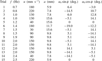
. To account for multiple local maxima, the routine was run as a series of local searches. Initial conditions were chosen to ensure a variety of relative strengths between initial parameters (table 3).
Initial positions in state space for the 15 optimization trials that converged on optima
 $\mathscr{A}_{\mathit{5D}}$
and
 $\mathscr{B}_{\mathit{5D}}$
.

At each iteration of the routine, five steps are taken in each dimension of
 $\mathscr{P}$
: two ‘small steps’ (defined below), two ‘large steps’, and one ‘null step’ (a step size of zero). After all dimensions have been considered, the steps that maximized efficiency are applied to the proposed solution. If a small step led to higher efficiency, the step size in that dimension is decreased; if a large step led to higher efficiency, the step size in that dimension is increased. This variable step size allows the search procedure to decelerate/accelerate and reduces the search time considerably.
The step sizes can be written as an
 $n\times 5$
matrix
 ${\it\Delta}$
, where the rows represent step sizes for
 $f$
(Hz),
 $u$
(
 $\text{mm}~\text{s}^{-1}$
),
 $a$
(mm),
 ${\it\alpha}_{0}\;\text{sin}\,{\it\phi}$
(deg.), and
 ${\it\alpha}_{0}\;\text{cos}\,{\it\phi}$
(deg.). Note that maximum pitch angle and phase offset were converted to rectilinear coordinates in the
 ${\it\alpha}_{0}{-}{\it\phi}$
plane. This avoids solutions getting stuck at
 ${\it\alpha}_{0}=0$
, an error that occurs because adding pitch can decrease efficiency when done over certain ranges of phase offset. The starting value of
 ${\it\Delta}$
was chosen to be
 $\langle 0.1,10,2,5,5\rangle \otimes \langle 0,-1/2,1/2,-2,2\rangle$
. Note the small steps (corresponding to entries with
 $\pm 1/2$
) and large steps (corresponding to entries with
 $\pm 2$
) in each dimension. Convergence was found to be stable above step sizes of
 ${\it\Delta}^{0}/4$
, so this value was used for the termination criterion of the routine. All trials reached this termination criterion in less than 20 steps. The details of the routine are given in pseudocode below:

Appendix B. Linear beam theory with added mass
Small deflections
 $d$
of a homogeneous panel with constant cross-section can be modelled by the linear beam equation (Weaver, Timoshenko & Young Reference Weaver, Timoshenko and Young1990),
 $$\begin{eqnarray}{\it\rho}_{p}{\it\delta}s\frac{\partial ^{2}d}{\partial t^{2}}+EI\frac{\partial ^{4}d}{\partial x^{4}}=\mathscr{F}_{\mathit{ext}},\end{eqnarray}$$
where
 ${\it\rho}_{p}$
is the density of the panel and
 $\mathscr{F}_{\mathit{ext}}$
is the external force per unit length. Following Ramananarivo, Godoy-Diana & Thiria (Reference Ramananarivo, Godoy-Diana and Thiria2013) and Quinn et al. (Reference Quinn, Lauder and Smits2014a
), we replace the mass per length of the panel,
 ${\it\rho}_{p}{\it\delta}s$
, with an effective mass per length,
 $\mathscr{M}{\it\rho}sc$
, where
 $\mathscr{M}$
is a constant to be fitted experimentally. This substitution incorporates added-mass forces into (B 1), which can be rewritten in dimensionless form as
 $$\begin{eqnarray}{f^{\ast }}^{2}\frac{\partial ^{2}D^{\ast }}{\partial {T^{\ast }}^{2}}+\frac{\partial ^{4}D^{\ast }}{\partial {X^{\ast }}^{4}}=\mathscr{F}_{\mathit{ext}}^{\ast },\end{eqnarray}$$
where
 $D^{\ast }\equiv d/a$
,
 $X^{\ast }\equiv x/c$
,
 $T^{\ast }\equiv t\,f$
, and
 $\mathscr{F}_{\mathit{ext}}^{\ast }\equiv \mathscr{F}_{\mathit{ext}}c^{4}/(ba)$
. In this modified equation,
 $\mathscr{F}_{\mathit{ext}}$
represents any forces in addition to added mass, such as internal damping or viscous drag.
A special case to consider,
 $\mathscr{F}_{\mathit{ext}}^{\ast }=0$
, represents conditions where added-mass forces dominate the dynamics of the flow. Along with our four boundary conditions, one end fixed (
 $D^{\ast }(0)=0$
,
 $D^{\ast ^{\prime }}(0)=0$
) and one end free (
 $D^{\ast ^{\prime \prime }}(1)=0$
,
 $D^{\ast ^{\prime \prime \prime }}(1)=0$
), the homogeneous case of (B 2) has closed-form eigenmodes. The eigenvalues
 $\hat{f_{n}^{\ast }}$
of the modes are determined implicitly as solutions to
 $$\begin{eqnarray}\text{cos}\sqrt{\hat{f_{n}^{\ast }}}\;\text{cosh}\sqrt{\hat{f_{n}^{\ast }}}=-1.\end{eqnarray}$$
In each mode, the actual eigenfrequency is
 $f_{n}=\hat{f_{n}^{\ast }}(b/(\mathscr{M}{\it\rho}sc^{5}))^{1/2}$
. A modal projection analysis of the panel in the current study shows that modes 3 and 4 are excited over the frequency range considered here (Quinn et al.
Reference Quinn, Lauder and Smits2014a
). The theoretical eigenvalues are
 $\hat{f_{3}^{\ast }}\approx$
62 and
 $\hat{f_{4}^{\ast }}\approx$
121, compared with the measured values of
 $\hat{f_{3}^{\ast }}\approx$
26 and
 $\hat{f_{4}^{\ast }}\approx$
53. The linear model over-predicts the eigenvalues, but the ratio between the two flexural frequencies,
 $\hat{f_{4}^{\ast }}/\hat{f_{3}^{\ast }}$
, is consistent with the model, differing from the predicted ratio by less than 5 %. This agreement implies that a simple added-mass constant can be fitted to the propulsor, after which the theory can predict additional eigenfrequencies. For example,
 $\mathscr{M}=1$
was chosen above to facilitate comparison with other studies, but choosing
 $\mathscr{M}=0.14$
brings both measured eigenfrequencies to within 4 % of their modelled values.