


1. Introduction
Around 121 million, or nearly half of the world’s annual pregnancies, are unintended (Bearak et al., Reference Bearak, Popinchalk, Beavin, Ganatra, Moller, Tunçalp and Alkema2022).Footnote 1 In its State of the World Population report, the UNFPA (2022) highlights this phenomenon as the world’s unseen crisis. Such unintended pregnancies present a pressing issue for many public health systems and economies.Footnote 2 According to the UNFPA report, a notable number of unintended pregnancies end in unsafe abortions, leading to 5–13% of maternal deaths worldwide. Moreover, a growing body of research also shows that unintended or unplanned births are associated with a range of unfavorable outcomes for children, mothers, siblings, and households overall (Barber & East, Reference Barber and East2011; Gipson et al., Reference Gipson, Koenig and Hindin2008; Lin & Pantano, Reference Lin and Pantano2014). Children born after unintended pregnancies are at a greater risk of experiencing lower developmental outcomes, attaining a lower level of education, and experiencing physical and mental health problems, due to suboptimal parental investment (Axinn et al., Reference Axinn, Barber and Thornton1998; Ebert & Vollmer, Reference Ebert and Vollmer2022; Le & Nguyen, Reference Le and Nguyen2022; Nguyen, Reference Nguyen2018).
Theoretically, we might expect this relationship to be more pronounced for girls for two related reasons. First, an unintended birth raises household size beyond what parents had planned for; as in the classic quantity-quality tradeoff, this dilutes resources across more children, and does so more sharply than a planned birth of the same order would, since the household has had no opportunity to budget for it in advance. Second, where resources are strained, parents in patriarchal settings may ration what remains along gender lines, favoring sons. Yet, empirical evidence on whether these penalties vary by child gender remains scarce.
In this paper, we ask whether children born after an unintended pregnancy have different cognitive outcomes than other children, and, if so, whether this difference varies by child gender. We do this in the context of Indonesia, where unintended pregnancies had reached approximately 36% of annual pregnancies nationally during the five-year period from 2015 to 2019 (Bearak et al., Reference Bearak, Popinchalk, Ganatra, Moller, Tunçalp, Beavin, Kwok and Alkema2020; Guttmacher Institute, 2022). While this figure is lower compared to the Southeast Asian regional average (45%), it is the highest in the region in absolute number terms. With Indonesia’s annual pregnancies at almost 8 million on average, nearly 3 million − or more than one-third − are unintended (Giorgio et al., Reference Giorgio, Utomo, Soeharno, Aryanty, Stillman, Philbin, Singh and Sedgh2020; Guttmacher Institute, 2022). Given the scale of unintended childbearing in Indonesia, even a modest gender-specific effect on children’s cognitive development could carry substantial implications at the population level.
Using rich data from five waves of the Indonesia Family Life Survey (IFLS), this paper offers important insights on the cognitive outcomes of Indonesian children born after unintended pregnancies. We match the data on maternal fertility preferences with data on subsequent birth outcomes to assign a birth intendedness status to each child. Linking that status to a wide range of children’s cognitive outcomes later in life, we exploit the random assignment of gender to isolate what we term the girl penalty: the cognitive disadvantage that girls, relative to boys, experience specifically when born after an unintended pregnancy. The results suggest that while girls outperform boys in most cognitive domains, being born after an unintended pregnancy carries a unique penalty that is only evident for girls, and makes no significant difference for boys. While we acknowledge that fertility intentions may be endogenous, our identification strategy specifically focuses on the interaction between unintendedness and gender. By doing so, we exploit the random assignment of child gender to isolate a causal “girl penalty” that exists independently of the factors driving pregnancy intentions. The results are robust to controlling for a wide range of child, parent, and household characteristics, as well as time-and location-fixed effects, and to potential omitted variable bias, as confirmed using the partial identification approach proposed by Oster (Reference Oster2019).
Our analysis also shows that the girl penalty in numerical and language abilities emerges in adolescence, but is not present at younger ages. This suggests that if parental investment varies by fertility intentions and gender, it shows in the longer term but not in the short run. This is consistent with earlier studies on children’s developmental trajectories, which show that early skills and parental investment lead to more established and visible competencies in the child’s later life (Cunha & Heckman, Reference Cunha and Heckman2007; Doyle et al., Reference Doyle, Harmon, Heckman, Logue and Hyeok Moon2017). Moreover, we explore the possibility that differences in parental investment by gender, within the group of unintended children, may be a potential mechanism behind our main results. We find evidence consistent with this channel: girls born after an unintended pregnancy are less likely to be enrolled in private schools and more likely to exhibit poorer health outcomes in early childhood, relative to boys born under the same circumstances; no comparable gap is evident among intended children.
This paper contributes to the literature in three important ways. First, as noted above, there are studies that link child unintendedness with suboptimal outcomes later in life (Axinn et al., Reference Axinn, Barber and Thornton1998; Le & Nguyen, Reference Le and Nguyen2022; Nguyen, Reference Nguyen2018), including Joyce et al. (Reference Joyce, Kaestner and Korenman2000), who establish an empirical link between unintended pregnancy and child health outcomes and development. However, the evidence that such a relationship varies by gender is lacking. Second, we add to the evidence on fertility and child development in Indonesia. Previous work, such as Jensen and Ahlburg (Reference Jensen and Ahlburg2002), has documented that children whose births were unintended by their mothers are more likely to experience illness and receive suboptimal medical care, while Calimeris and Peters (Reference Calimeris and Peters2017) shows that later-born children in Indonesia are disadvantaged in household resource allocation and perform worse on cognitive tests. Other Indonesian evidence includes Suryadarma (Reference Suryadarma2013), who documents the gender gap in cognitive outcomes, and Palloni (Reference Palloni2017), who shows that children born of non-preferred gender experience poorer health. We extend this evidence by showing that these penalties are sharply gendered, falling specifically on girls born after an unintended pregnancy. Third, our results contribute to the emerging evidence on the “girl penalty” in developing contexts more broadly. An important related study is Ebert and Vollmer (Reference Ebert and Vollmer2022), who use an Indian community case study to establish the presence of a cognitive development penalty among girls of son-preferring parents. However, they do not explore this relationship in the context of child unintendedness as we do in this paper. Our findings are also consistent with Hazan and Zoabi (Reference Hazan and Zoabi2015)’s theoretical mechanism, in which parents with a preference for sons keep having children until a son is born; because this means daughters are systematically born into larger families than sons, they experience a quantity-quality-based disadvantage in human capital even without any direct discrimination in resource allocation. We provide direct empirical evidence for this channel operating through unintended childbearing specifically.
We organize the rest of the paper as follows. In Section 2, we provide a conceptual framework and discuss the Indonesian context. In Section 3, we discuss the data used in the analysis and provide descriptive statistics. Section 4 presents the empirical approach, while Section 5 reports the results of our analysis and robustness checks. Section 6 concludes the paper.
2. Conceptual framework and Indonesian context
2.1. Parental investment and child cognitive development
Parental investments are a key factor in children’s cognitive development and human capital accumulation (Aizer & Cunha, Reference Aizer and Cunha2012; Attanasio, Reference Attanasio2015; Cunha & Heckman, Reference Cunha and Heckman2007;). Cognitive ability, as a brain-based skill, encompasses both fluid and crystallized intelligence, playing a fundamental role in child development and future economic outcomes (Acosta & Muller, Reference Acosta and Muller2018; Acosta et al., Reference Acosta, Muller and Sarzosa2015). Household decisions regarding the allocation of resources to individual children can vary significantly according to specific child characteristics, such as birth order, gender, and intendedness (Abufhele et al., Reference Abufhele, Behrman and Bravo2017; Pavan, Reference Pavan2016; Pollak, Reference Pollak2002).
Gender remains one of the most significant factors shaping parental preferences. The literature on son preference, particularly in patrilineal societies, highlights an economic rationale for investing in boys, who often provide greater old-age support or inherit family assets (Levine & Kevane, Reference Levine and Kevane2003; Rammohan & Vu, Reference Rammohan and Vu2018). Consistent with this economic framing, evidence from China shows that when women’s relative earning potential rises, discriminatory treatment of girls declines: exogenous increases in female income improve girls’ survival rates and raise educational attainment for all children, whereas increases in male income specifically reduce girls’ educational attainment (Qian, Reference Qian2008). In contexts like India, studies show that girls may receive shorter periods of breastfeeding or lower educational investment as parents prioritize resources for sons (Choi & Hwang, Reference Choi and Hwang2000; Jayachandran & Kuziemko, Reference Jayachandran and Kuziemko2011).
Unintended childbearing can further exacerbate these disparities by causing disruptions in household capacity for human capital investment. This works through two related channels. First, an unintended birth increases the number of children in the household, which, following the classic quantity-quality tradeoff formalized by Becker and Lewis (Reference Becker and Gregg Lewis1973), reduces the resources available per child as a fixed household budget is spread across more offspring (Anukriti et al., Reference Anukriti, Bhalotra and Tam2016; Lee, Reference Lee2007). Since an unintended birth by definition occurs after a mother’s desired fertility has already been met, unintended children are typically higher-parity, later-born children who must share this budget with more siblings than their intended counterparts (Cáceres-Delpiano, Reference Cáceres-Delpiano2006; Conley & Glauber, Reference Conley and Glauber2005). Second, and beyond this pure size effect, the constraint imposed by an unintended birth is more binding than that imposed by a planned birth of the same order, precisely because the household has had no opportunity to anticipate and budget for it in advance − through adjusted savings, labor supply, or birth spacing. Quasi-experimental evidence using twin births as an instrument for family size shows that birth order specifically carries a robust, causal educational penalty even in settings where the effect of family size alone is small (Black et al., Reference Black, Devereux and Salvanes2005). In developing-country settings more comparable to Indonesia, similar quasi-experimental designs show that an additional child significantly reduces siblings’ schooling progress, expected college enrollment, and health (Rosenzweig & Zhang, Reference Rosenzweig and Zhang2009). This channel is also consistent with the formal mechanism in Hazan and Zoabi (Reference Hazan and Zoabi2015), who show theoretically that when parents prefer sons and therefore keep having children until they have one, daughters are, on average, born into larger families than sons, generating a quantity-quality-based gender gap in human capital even before any direct discrimination in resource allocation takes place.
In societies with gender-biased preferences, daughters born after unintended pregnancies may experience a “double disadvantage” from both increasing family size and discriminatory resource allocation (Kugler & Kumar, Reference Kugler and Kumar2017). By contrast, intended births are typically planned within the household’s existing resource capacity; because budget constraints are less binding in these cases, parents face less pressure to ration investments along gender lines, which is why we expect any gender-based cognitive penalty to be concentrated among unintended children. While some evidence exists for these dynamics in India (Ebert & Vollmer, Reference Ebert and Vollmer2022), it remains unclear whether similar patterns hold in other sociocultural settings.
2.2. Gender norms and fertility in Indonesia
Indonesia offers a unique context for studying these relationships. While girls in Indonesia generally outperform boys on cognitive development indicators (OECD, 2019), the country remains a patriarchal society where cultural and religious norms shape gender roles. Indonesian Islam is nonetheless generally considered more moderate than the patriarchal interpretations of Islamic law found in some South Asian and North African contexts (Ebadi, Reference Ebadi2003; Kazemi, Reference Kazemi2000). Traditional values, codified in Law 1/1974, often assign men the role of breadwinners and women that of homemakers, potentially creating economic incentives for preferential treatment of sons when resources are rationed, as is disproportionately the case following an unintended pregnancy (Hatton et al., Reference Hatton, Sparrow, Suryadarma and van der Eng2018; Jensen & Ahlburg, Reference Jensen and Ahlburg2002).
Unlike some South Asian contexts, son preference at birth is not directly observed in Indonesia’s aggregate sex ratios (Guilmoto, Reference Guilmoto2015). Indeed, Indonesia’s sex ratio at birth remained within the biologically “natural” range of approximately 105 boys per 100 girls as of 2020. This is consistent with survey-based evidence finding no clear pattern of “missing daughters” in Indonesian birth spacing and nutrition outcomes, although gender gaps in educational attainment and inheritance have historically persisted (Kevane & Levine, Reference Kevane and Levine2000). Son preference nonetheless continues to shape fertility behavior directly: nationally representative survey data show that having only daughters is a strong predictor of a woman’s intention to continue childbearing (Abang Ali & Arabsheibani, Reference Abang Ali and Arabsheibani2020), one of the channels through which son preference can give rise to unintended pregnancies in the first place. However, reproductive choices are heavily constrained; abortion is almost entirely illegal, and access to effective contraception remains limited (Giorgio et al., Reference Giorgio, Utomo, Soeharno, Aryanty, Stillman, Philbin, Singh and Sedgh2020; Landiyanto, Reference Landiyanto2009). These constraints lead to high rates of unintended pregnancy, which is often contextualized within community values where every child born (especially in marriage) is seen as a “blessing” (Jensen & Ahlburg, Reference Jensen and Ahlburg2002).
Despite this apparent lack of prenatal sex selection, research has shown that children of a non-preferred gender in Indonesia experience poorer health outcomes and higher rates of illness (Jensen & Ahlburg, Reference Jensen and Ahlburg2002; Palloni, Reference Palloni2017). Our study extends this literature by examining how the interaction between fertility intentions and gender norms shapes long-term cognitive outcomes, exploiting the random assignment of gender to isolate a causal girl penalty among children born after unintended pregnancies.
3. Data
3.1. Source
This paper uses data from the Indonesia Family Life Survey (IFLS) – a rich longitudinal survey conducted by RAND Corporation, USA, in collaboration with Survey Meter Indonesia. IFLS contains the key measures of relevance to this study: a wide range of children’s cognitive outcomes alongside mothers’ fertility preferences. Additionally, IFLS offers information on a wide set of background socioeconomic characteristics of children and their households. The survey has five different waves, spanning from 1993 to 2015, although not conducted at regular intervals.Footnote 3 It represents over 80% of Indonesia’s population, covering 13 out of 30 provinces in the most populated regions of West Indonesia. The excluded provinces are predominantly located in remote Eastern regions of Indonesia (e.g., Papua, Maluku, and parts of Sulawesi and Kalimantan), which are generally more rural, potentially more traditional, and economically disadvantaged; thus, our findings may represent a conservative estimate of the gender-based unintendedness penalty. One of IFLS’s prominent features is following up with respondents who moved and extended their households, resulting in a low inter-survey attrition rate (Frankenberg et al., Reference Frankenberg, Smith and Thomas2003, Reference Frankenberg, Suriastini and Thomas2005). The dataset employed in our analysis is cross-sectional; we utilize the panel feature of IFLS primarily to follow the history of maternal fertility and capture information on children born after the elicitation of maternal fertility intentions.
3.2. Variables
3.2.1. Measures of child cognitive outcomes
This study examines how mothers’ fertility preferences and child gender jointly shape the child’s numerical and literacy competencies by considering the cognitive outcome domains spanning two main types of human intelligence − fluid and crystallized intelligence. Information about children’s numerical and language skill accumulation is drawn from two sources: cognitive tests administered during the IFLS survey, and respondents’ recalled scores on national examinations (EBTANAS/UAN/UN).Footnote 4
IFLS introduced cognitive ability tests in its third wave in 2000 through the questions in modules EK1 and EK2. Since then, these modules have been widely used in studies investigating cognitive ability in Indonesia (Botzet et al., Reference Botzet, Rohrer and Arslan2020; Calimeris & Peters, Reference Calimeris and Peters2017; Cameron et al., Reference Cameron, Chase, Haque, Joseph, Pinto and Wang2021). Both test modules are similar in structure and type of questions. However, they are different in difficulty level, with EK2 considered more advanced than EK1 (Suryadarma, Reference Suryadarma2013). EK1 targets respondents aged 7−14 years or those who are illiterate or not attending school. In comparison, EK2 targets respondents aged 14−24 years, and those who have already done EK1 in the preceding waves. A respondent of EK2 who has ever taken EK1 in the previous wave will be asked to do EK1 again along with EK2 (Strauss et al., Reference Strauss, Witoelar and Sikoki2016). Given these preconditions, the age of the EK1 respondents can be over 14 years old when undertaking the repeated EK1; similarly, EK2 respondents can be over 24 years old.
We consider both EK1 and EK2 modules in constructing the outcomes of interest in our study, and we conduct estimations in separate sub-samples of individuals defined by EK1 vs EK2 test type. For the EK1 sub-sample, we impose an age restriction by only including those who are still in the original target age range of the test (7–14 years) − that is, those who have done the test for the first time and those who repeat the test when they are still under 14. The low level of difficulty − especially for test takers at higher ages − has been our rationale to apply this procedure in addition to getting a clear age division between the two modules and sub-samples. Additionally, this age-based restriction affords the opportunity to see whether the potential differences in cognitive development associated with child unintendedness and gender status vary at different stages of a child’s development.
EK1 consists of twelve questions while EK2 has eight questions for Raven’s Visuospatial test. Both modules contain five numerical questions assessing numerical reasoning abilities. Visuospatial ability supports and is closely related to numeracy and language (see Fanari et al., Reference Fanari, Meloni and Massidda2019; Georges et al., Reference Georges, Cornu and Schiltz2021). Raven’s visuospatial test administered by IFLS in modules EK1 and EK2 is an abridged version of Raven’s Progressive Matrices, which is a non-verbal test in which each question contains visual geometric shapes with a missing part. Respondents are asked to choose among the four answer choices which shape is the most appropriate to fill in the missing part (Schroders et al., Reference Schroders, Dewi, Nilsson, Nichter and San Sebastian2020; Strauss et al., Reference Strauss, Witoelar and Sikoki2016). The Numerical Reasoning test, in turn, consists of five questions in both modules − EK1 and EK2. The basic difference that makes the test for this skill more difficult in EK2 is that in EK2 the questions regarding addition, subtraction, division, and multiplication are more complex than in EK1. For instance, while EK1 might include simple additions, EK2 includes questions such as serial subtractions (e.g., 100 − 7) and more complex multi-step problems. In addition, in EK2, two of the five questions are in the form of math word problems (e.g., calculating change from a transaction). Similar to the Raven’s visuospatial test, the Numerical Reasoning test is a written test and provides the respondents with three to four options of answers to choose from.Footnote 5 Raven’s Visuospatial test result has been recognized as the proxy of fluid intelligence, while Numerical Reasoning is used as the proxy for assessing crystallized intelligence (see Gaduh & Singhal, Reference Gaduh and Singhal2021; Kusumawardhani et al., Reference Kusumawardhani, Suryadarma, Veto and Indrio2019;). The Raven’s Visuospatial and Numerical Reasoning test results sum to a total score used to proxy general cognition (see e.g., Cameron et al., Reference Cameron, Chase, Haque, Joseph, Pinto and Wang2021).
We additionally consider the Descending Subtraction test in the list of cognitive indicators, taking advantage of the availability of additional cognitive assessments in the last wave of IFLS. Adding this test also allows us to examine the children’s cognitive performance in different types of tests based on their delivery methods. Unlike IFLS’s other numerical tests, Descending Subtraction is delivered verbally and relies on auditory memory to test the respondent’s concentration and mental intactness essential to performing arithmetic operations (Attout & Majerus, Reference Attout and Majerus2018; Bristow et al., Reference Bristow, Angela Jih, Slabich and Gunn2016; Starkey & McCandliss, Reference Starkey and McCandliss2014;). In this test, respondents are asked to count down from one hundred by seven five times. The test is scored based on the total number of correct subtractions, resulting in a score ranging from 0 to 5.
Finally, math and Indonesian language exam scores are used to measure cognitive abilities in the numeric and literacy domains. Exam score results have been available since the first wave of IFLS for all levels of education − primary, junior high, and high school. The rationale for selecting the two subjects is that they are the most relevant to both numerical and language dimensions of cognition. Besides, math and the Indonesian language are the only subjects consistently tested in national exams; thus, the data are consistently reported in the IFLS.Footnote 6 The number of subjects in which scores are asked in the IFLS questionnaire varies from wave to wave, along with the changes in national exam policies.Footnote 7 It is important to note that we use only the exam score from the elementary school level. The main rationale for opting for the elementary school level is the limited number of observations from junior high school and high school − a situation that can be explained by low years of schooling.Footnote 8 Hence, the exam scores sample represents respondents in the early adolescent age range.
We sum the correct answers of each cognitive test resulting in a 0−5 score scale for Numerical Reasoning EK1 and EK2 and Descending Subtraction test, 0−8 score scale for Raven’s Visuospatial EK2, 0−12 score scale for Raven’s Visuospatial EK1, 0−13 score scale for General Cognitive EK2, and 0−17 score scale for General Cognitive EK1; and use readily available final exam scores to indicate cognitive abilities. These differences in the score scales pose a challenge to the interpretation of the results; thus, we standardize the score by subtracting each score from the sample mean and dividing it by the standard deviation.
Table A.1 in the Supplementary material summarizes the cognitive indicators used in this study. Each cognitive test may describe multiple abilities and cover a variety of cognition domains. The Numerical Reasoning test in EK modules and Math Exam score can also explain the respondents’ language literacy, as several of its questions are delivered in the form of math word problems. Similarly, not only does Descending Subtraction capture arithmetic and computational skills, but it is also widely used to measure mental state.
3.2.2. Estimation samples
The sample used in our study is constructed from the initial pool of 25,972 children covered across IFLS survey waves. We restrict this to children born between waves 1 (1993) and 5 (2015) with available maternal fertility preference information who were still living in the same household as their mothers at the time of the survey − totaling 6,842 observations. If we restrict our sample to children without missing information on cognitive outcomes and control variables, the sample size drops to 6,002 observations. Because the cognitive outcome measures available in IFLS differ by children’s age and educational stage, with younger children taking the EK1 module, older youth the EK2 module, and another group identified through their recalled national examination scores, this overall sample naturally subdivides into three estimation sub-samples:
-
1. Youth Cognitive Sample (YCS): Comprises 986 respondents, typically aged 15–24, whose cognitive outcomes are measured using the more advanced EK2 module (Raven’s Visuospatial, Numerical Reasoning, and General Cognitive scores) as well as the Descending Subtraction test.
-
2. Elementary Exam Sample (EES): Comprises 1,558 respondents (for mathematics) and 1,563 respondents (for Indonesian language), whose cognitive outcomes are measured using recalled scores on the national elementary school final examination (EBTANAS/UAN/UN), sat at approximately 11–14 years of age.
-
3. Child Cognitive Sample (CCS): Comprises 3,458 respondents aged 7–14, whose cognitive outcomes are measured using the EK1 module (Raven’s Visuospatial, Numerical Reasoning, and General Cognitive scores).
Evaluating these three distinct sub-samples allows us to investigate cognitive performance across different developmental stages (childhood vs. youth) and cognitive evaluation approaches (direct survey-administered tests vs. national standardized examinations).
The restrictions imposed on the sample are based on the information regarding key variables of interest in the model, and are therefore necessary. However, they may raise concerns over potential selection bias. In Table A.2 in the Supplementary material we report the means (and standard deviations) of variables in our estimation samples and those dropped due to missing data on key variables of interest, and the associated differences. As seen from the table, the overall characteristics of the estimation samples are not too different from those in the dropped samples, with most similarities observed in the case of the Youth Cognitive Sample where we observe a large difference in the age of the children only. For the Elementary Exam and Child Cognitive Samples, some differences between estimation and dropped observations are statistically detectable, yet the magnitudes are generally small and unlikely to reflect systematic selection along the key dimensions of this study. Overall, the pattern of balance across samples provides reasonable reassurance that sample attrition due to missing data does not introduce substantial selection bias into our estimates.
3.2.3. Measures of maternal fertility preferences
Information on maternal fertility preferences is taken from module 4 of the IFLS, which collects the histories of marriage and pregnancies.Footnote 9 Using this module, we follow the maternity history of ever-married women aged 15−49 from wave 1 to wave 4 of IFLS. We draw on respondents’ (Yes/No) answers to: “Do you wish to have another child (besides the children you already have)?” We match this information with the information on children born after the elicitation of the mother’s preference, to assign unintendedness status to each child. Specifically, for each wave in which a mother’s fertility preference is elicited, we identify all children subsequently born to her, and among these we identify the first birth occurring after that particular elicitation; this child’s unintendedness status is then assigned based on the preference recorded at that elicitation.
In our final estimation samples, unintended children make up 32% of the Youth Cognitive Sample (YCS), 30% of the Elementary Exam Sample (EES), and 29% of the Child Cognitive Sample (CCS) (see Appendix Table A.3 in the Supplementary material). At the mother level, a somewhat smaller share of mothers have given birth to at least one unintended child: approximately 30% in the YCS, 28% in the EES, and 26% in the CCS. While preferences could technically shift between survey waves, such instances are rare in our data. For example, among mothers with unintended children, the “unintended” status is highly consistent across births: approximately 94% (YCS), 90% (EES), and 80% (CCS) of their children born after the initial “no more” preference was elicited are indeed unintended. This high within-mother consistency also implies limited variation for reliably exploiting mother fixed effects: only around 114 mothers in the YCS and 260 in the EES have children of different intendedness statuses. As a result, the IFLS dataset employed in our analysis is cross-sectional, and we only utilize the panel feature primarily to follow the history of maternal fertility and capture information on children born after the elicitation of maternal fertility intentions. This allows us to maximize sample size and consistency.
As a consequence, a mother may appear more than once in our dataset depending on the number of pregnancies and fertility preferences elicited over the period from wave 1 to wave 4 of IFLS. Likewise, the same child may appear in multiple waves after the mother’s fertility preference is elicited. In these cases, we record the associated outcome as of the latest survey wave in which it was observed.
3.2.4. Measures of potential transmission mechanisms
Our analysis of mechanisms focuses on two forms of parental investment in children’s human capital: education and health. Table A.1 in the Supplementary material presents the list of relevant variables.
The literature on economic returns to education has pointed to the importance of educational inputs in the child’s early life cycle (Ashenfelter & Krueger, Reference Ashenfelter and Krueger1994; Hanushek & Woessmann, Reference Hanushek and Woessmann2008). Additionally, Attanasio et al. (Reference Attanasio, Meghir and Nix2020) highlight the effect of parental preference and school quality on children’s outcomes (Attanasio et al., Reference Attanasio, Meghir and Santiago2012). We measure investment in education by employing, in the first instance, a dummy variable that distinguishes between enrollment in private (vs public) school. The parental decision to enroll their children in private schools may be motivated by a number of considerations, including the aspiration to seek quality education or a strategy for ensuring schooling continuity. Private schools in Indonesia are diverse, including private religious institutions (such as Madrasahs or Christian schools) and international schools that may offer English-language instruction or specialized facilities. Enrollment in private schools has been used in several studies investigating child quantity-quality tradeoffs, including Conley and Glauber (Reference Conley and Glauber2005) and Cáceres-Delpiano (Reference Cáceres-Delpiano2006) who proxied for parental investment in children using private school enrollments. Additionally, we use a dummy variable to measure whether a child is enrolled in a school (regardless of the type of school enrolled in).
Parental investment in early child health, encompassing resources and the quality of childrearing provided by parents, determines children’s survival and their health in later life (Jayachandran & Kuziemko, Reference Jayachandran and Kuziemko2011; Palloni, Reference Palloni2017). Parental investment in children’s early health plays an important role in shaping children’s health outcomes at school age (Pruckner et al., Reference Pruckner, Schneeweis, Schober and Zweimüller2021) and adulthood (Currie, Reference Currie2009). We measure parental investment in children’s health through two sets of outcomes. First, we consider direct measures of investment, including basic immunization and antenatal care visits. Second, we look at early childhood health outcomes which likely capture the different ways parents contribute to children’s outcomes more completely. Specifically, we consider whether the child experienced, at any point between ages 0 and 15, a severe illness that required being bedridden or hospitalized, or a diagnosis of asthma. Our rationale for utilizing early childhood health outcomes is that early life serves as a critical period in a child’s life, and health outcomes during this time reflect the quality of parental childrearing (Palloni, Reference Palloni2017). Asthma is specifically included as it is a common chronic condition in Indonesia that can be sensitive to environmental stressors and quality of early medical care, thus serving as a proxy for sustained parental investment in a child’s health environment.
3.2.5. Control variables
In addition to child unintendedness status and gender (captured through a dummy that takes 1 for a girl and 0 for a boy) and the interaction of the two, we control for background characteristics of individuals, their parents and their household structure, following the literature on maternal fertility preferences and child outcomes (Ebert & Vollmer, Reference Ebert and Vollmer2022; Palloni, Reference Palloni2017; Suryadarma, Reference Suryadarma2013;). These include child age in years, number of older brothers, and number of older sisters. Controlling for the number of existing siblings is particularly important given the evidence from existing studies showing that unintended children are likely to be later-born children (see Ebert & Vollmer, Reference Ebert and Vollmer2022; Jayachandran & Kuziemko, Reference Jayachandran and Kuziemko2011). Thus, additional older brothers and sisters variables are added to mitigate the bias that may arise due to parents’ preferences for older children and for a particular gender (see Calimeris & Peters, Reference Calimeris and Peters2017).
Household wealth is proxied using the total value of household assets, following Black et al. (Reference Black, Devereux and Salvanes2007) and Huang (Reference Huang2013). This measure, obtained from the detailed asset module in IFLS, aggregates the reported market value of various asset categories including housing, land, vehicles, livestock, and jewellery. To ensure comparability across waves, we deflate these values to the 2021 price level using the consumer price index (CPI) from the Indonesian Central Bureau of Statistics. We additionally account for differences in parental endowment, including mother’s age when the child was born as well as mother’s and father’s years of schooling, which are widely used in previous studies examining children’s learning outcomes and shown to have significant effects (Giménez-Nadal & Molina, Reference Giménez-Nadal and Alberto Molina2012; Hornby & Lafaele, Reference Hornby and Lafaele2011). Suryadarma (Reference Suryadarma2013) shows that learning outcomes are lower in students from an Islamic religious background, and our models account for this observation by including a dummy that takes 1 if the mother’s religion is Islam. Finally, we follow Palloni (Reference Palloni2017) to include the year and month of childbirth, provincial and rural-urban location, and year of IFLS wave indicators among the controls. Appendix Table A.1 in the Supplementary material provides a complete description of the control variables used in the study.
For respondents who took cognitive tests, control variables are drawn from the same survey wave as the outcome (e.g., outcomes from wave five are linked to controls from wave five). For respondents who report elementary school exam scores, we instead align the controls as closely as possible to the conditions at the time the exam was taken: specifically, child age and household size are adjusted to correspond to the year in which the child sat the elementary school final examination, rather than the survey wave in which the score was reported.
By using contemporaneous covariates in our default approach, we aspire to accurately capture the conditions that may impact child outcomes. Since the outcomes in our model are assessed during early to mid-adolescence, there can be substantial time gaps between when mothers were surveyed and when children took or reported their cognitive test and exam scores (of up to 220 months for some samples). However, the use of contemporaneous controls may give rise to some theoretical concerns. For example, assets or household size may be affected by unintended childbearing if families adjust their labor supply or resource allocation to accommodate an additional child; conversely, low household assets may increase the likelihood of unintended births due to restricted access to family planning services. Similarly, child gender might influence parental investment decisions and asset accumulation in patriarchal households. To mitigate such concerns, we take two approaches. First, in our baseline specifications, we take the approach of gradually adding various sets of controls as a way to gauge the sensitivity of the results to the presence of different (including potentially endogenous) controls. Second, we re-run models with controls measured at the time when mothers’ fertility preferences were elicited (Appendix Table A.9 in the Supplementary material).
3.3. Descriptive statistics
Table 1 presents the summary statistics of the background characteristics of children and their parents in the joint sample, by child gender and pregnancy intendedness status. We also report t-test statistics for the difference in means between intended and unintended children within each gender group. The descriptive statistics show that unintended children of both genders tend to have a larger number of older brothers and sisters, and are born to older mothers (by 4.2 years for girls and 4.8 years for boys), a pattern consistent with the fact that unintended children are, by construction, born after a mother has expressed a desire for no more children (see Table A.4 in the Supplementary material for the full breakdown across sub-samples). This mechanical birth-order relationship also explains the high within-mother consistency of unintendedness status reported in Section 3.2.3: once a mother’s desired family size is reached, children born after that point are almost always unintended, while the small minority of intended children in these mothers’ households are, by construction, those born earlier in the birth sequence.
Summary statistics of background characteristics by child gender and intendedness status (joint sample)

Table 1. Long description
The table presents summary statistics of background characteristics for children and their parents, categorized by child gender and pregnancy intendedness status. It includes data for both girls and boys, with columns for intended and unintended pregnancies, and the difference between them. The table has 12 rows and 6 columns. Row labels include Child age, Older brothers, Older sisters, Mother’s age at child birth, Mother’s education, Father’s education, Mother is Muslim, Household size, Household assets, and Urban location. Column headers are Intended, Unintended, and Diff. for both Girls and Boys. Each cell contains numerical values with standard deviations in parentheses and differences between intended and unintended pregnancies. Notable trends include higher numbers of older brothers and sisters for unintended children, and older maternal age at birth for unintended children.
Notes: Columns present the means and standard deviations of control variables for intended and unintended children, and their differences with associated significance levels. Standard deviations are shown in parentheses under the means. The sample size of each group matches the joint sample constructed by de-duplicating the analysis samples (
 $N=\mathrm{3,584}$
). ***p < 0.01; **p < 0.05; *p < 0.1.
Furthermore, parents of unintended children have significantly lower years of schooling. Specifically, mothers of unintended girls have 1.5 fewer years of schooling than mothers of intended girls, while mothers of unintended boys have 1.3 fewer years than their intended counterparts. A similar pattern holds for fathers: fathers of unintended girls have 1.1 fewer years of schooling, and fathers of unintended boys have 1.0 fewer years than their respective intended counterparts. Total household members are also significantly higher for unintended children, while there are no statistically significant differences in household assets or urban/rural residency by intendedness status.Footnote 10 These differences across intendedness and gender groups reinforce the importance of including these variables as controls in the regressions. However, we do not find significant differences when comparing children with the same intendedness status based on their gender, as reported in Table A.5 in the Supplementary material.
The summary statistics for all variables, including outcome measures, transmission mechanisms, and controls, across our three estimation sub-samples (YCS, EES, and CCS) are presented in Table A.3 in the Supplementary material. This table highlights the distinct developmental stages captured by each sub-sample, spanning late adolescence/youth in the YCS (mean age 17.2 years), early adolescence in the EES (mean age 12.4 years), and middle childhood in the CCS (mean age 10.9 years). Across all three sub-samples, the share of unintended children remains remarkably stable at around 30% (29.4% in CCS, 29.8% in EES, and 31.9% in YCS), with girls comprising approximately 47–49% of respondents. Regarding parental investments, private school enrollment increases markedly with educational level (rising from 12–14% at the elementary level to 40% in senior high school), while early-life health investments are generally high, with 75–81% of mothers receiving antenatal care and 54–66% of children obtaining basic immunizations.Footnote 11
Appendix Table A.6 in the Supplementary material presents the cognitive outcomes by child gender and unintendedness status and their differences in means. The results show that in the sub-sample of girls, there are significant differences in a number of cognitive outcomes in favor of intended girls. Relative to intended girls, unintended girls score 0.301 standard deviation units lower on the Numerical Reasoning test and 0.637 on the General Cognitive score. Furthermore, intended girls score 0.623 standard deviation units above their unintended counterparts on the Descending Subtraction Test. These tests are recorded at ages 15 and above and capture the possible consequences of unintendedness at adolescence. However, no significant differences by intendedness status are observed for tests undertaken by girls at ages 7–14. Similarly, we see hardly any significant differences in cognitive outcomes by intendedness status in the sample of boys.Footnote 12 Overall, the descriptive analysis presented in Appendix Table A.6 in the Supplementary material suggests that intendedness status may have implications for longer-term cognitive outcomes for girls but not boys. We explore this further in a regression analysis presented in the next section.
4. Empirical strategy
4.1. Baseline model
This study examines whether children’s cognitive outcomes differ according to their mothers’ fertility preferences, and, if so, whether this difference varies by child gender. Our empirical framework is designed to isolate this gender-specific difference − the girl penalty introduced above. To do that, we estimate a model of the following form:
 $$Co{g}_{im}={\beta }_{0}+{\beta }_{1}UN{D}_{im}\times GIR{L}_{im}+{\beta }_{2}UN{D}_{im}+{\beta }_{3}GIR{L}_{im}+{\beta }_{4}{X}_{im}+{\epsilon }_{im}$$
where
 $Co{g}_{im}$
is a marker of cognitive outcome of child
 $i$
born to mother
 $m$
,
 $UN{D}_{im}$
is an indicator for whether a child is born after an unintended pregnancy,
 $GIR{L}_{im}$
is an indicator of child gender,
 ${X}_{im}$
represents a vector of controls, and
 ${\epsilon }_{im}$
is the error term.
Equation (1) is estimated using OLS with standard errors clustered at mother level. While child unintendedness status may be endogenous, child gender is generally considered to be randomly assigned. Therefore, our primary coefficient of interest,
 ${\beta }_{1}$
, identifies the causal effect of being a girl (relative to a boy) among children who are born unintended. This framing allows us to isolate the gender-based penalty that manifests specifically when mothers’ fertility preferences are not met. We also report the significance of the sum of coefficients
 ${\beta }_{1}$
and
 ${\beta }_{2}$
to provide a total estimate of the impact for the girl group, but we treat the interaction term
 ${\beta }_{1}$
as the primary parameter of interest due to its cleaner identification based on child gender randomness.
We estimate equation (1) in three sub-samples corresponding to types of cognitive abilities captured at different stages of children’s lives (the Youth Cognitive Sample, the Elementary Exam Sample, and the Child Cognitive Sample).
4.2. Identification concerns
As noted in the descriptive analysis, there are notable differences in baseline characteristics between intended and unintended children. To address potential selection on observables and ensure comparability between the two groups, we employ entropy balancing (Hainmueller, Reference Hainmueller2011) as a robustness check. This method reweights the control group (intended children) to construct a synthetic control group whose covariate distribution matches that of the treatment group (unintended children). Specifically, we first compute sample weights that satisfy the balance constraints (requiring equal covariate means across groups) and then re-estimate equation (1) incorporating these weights.
While the matching approach mitigates the concerns over selection on observables, our empirical setup additionally raises questions around unobserved heterogeneity. It is possible, in particular, that parents who have unintended children are different from parents who do not have unintended children and treat boys and girls differently; but this does not need to be due to the fact that their children are unintended but due to unobserved characteristics or attitudes that correlate with having unintended children. Ideally, we would estimate models with mother fixed effects, which would mitigate the concerns over unobserved family-level confounders. However, such estimation would be reliant on the presence of a sufficiently large number of siblings sharing the same mother yet different in their intendedness status. The number of such siblings is small in our baseline samples − 114 in the Youth Cognitive Sample and 260 in the Elementary Exam Sample – making this approach hardly viable in the current setup.Footnote 13 Moreover, while the inclusion of mother fixed effects would have allowed us to address important sources of unobserved heterogeneity, it would not have served to entirely mitigate the concerns over omitted variable bias.
In the absence of a convincing approach to address the issue of unobserved heterogeneity in our setup (i.e., a valid instrumental variable), we adopt a partial identification approach proposed by Oster (Reference Oster2019) to assess the extent of bias from unobservables. We calculate the bias-adjusted coefficient derived by Oster (Reference Oster2019) as follows:
 $${\beta ^{\rm{*}}} \approx \tilde{\!\beta} - \delta{[\,\dot {\!\beta} } - \tilde{\!\beta} ]{{{R_{{\rm{max}}}} - \tilde R} \over {\tilde R - \dot R}}$$
where
 $\dot{\beta }$
and
 $\dot{R}$
and
 $\tilde \beta$
and
 $\tilde R$
are the coefficients and the R-squared from a regression with the treatment only, and treatment and controls, respectively,
 $\delta $
measures the relative importance of observables relative to unobservables in generating bias and
 ${R}_{\mathrm{m}\mathrm{a}\mathrm{x}}$
is the R-squared from a hypothetical regression that controls for observables and unobservables. Following Oster (Reference Oster2019), we set
 ${R}_{\mathrm{max}}=\mathrm{min} \left\{1.3 \tilde{R},\mathrm{}\mathrm{}1\right\}$
and estimate the bounds
 $[\tilde \beta, {\beta ^{\rm{*}}}]$
under an assumption of
 $\delta =1$
.
5. Results
5.1. Baseline results
As described in Section 3.2.2, our analysis relies on three distinct estimation sub-samples. We present the main results for the adolescent group (the Youth Cognitive Sample and Elementary Exam Sample) in the main text, while the results for younger children (the Child Cognitive Sample) are presented in Appendix Table A.8 in the Supplementary material.
Tables 2 and 3 present the implications of child gender and unintendedness status on different types of cognitive outcomes for the Youth Cognitive Sample and the Elementary Exam Sample, respectively. Each panel refers to a distinct cognitive outcome. The columns sequentially introduce additional covariate sets: child characteristics (column 2), parental background (column 3), household variables (column 4), province fixed effects (column 5), and birth cohort and survey wave fixed effects (column 6).Footnote 14 Column 7 presents a more restricted specification that retains only predetermined, child-invariant controls, excluding household variables that may themselves be affected by unintended childbearing. The gradual inclusion of covariates allows us to assess the sensitivity of our estimates to the addition of controls, some of which may be endogenous.
Girl penalty in cognitive tests administered for persons aged 15 and above, Youth Cognitive Sample (YCS)

Table 2. Long description
A table with seven columns and multiple rows, presenting the implications of child gender and unintendedness status on different types of cognitive outcomes for the Youth Cognitive Sample. Each panel refers to a distinct cognitive outcome. The columns sequentially introduce additional covariate sets: child characteristics, parental background, household variables, province fixed effects, and birth cohort and survey wave fixed effects. Column 7 presents a more restricted specification that retains only predetermined, child-invariant controls, excluding household variables that may themselves be affected by unintended childbearing. Row 1: Raven’s visuospatial EK2, Unintended, -0.225 (0.135); Unintended * Girl, 0.013 (0.087); Girl, -0.007 (0.076); Mean of dependent variable, 5.955; Observations, 983; R-Squared, 0.006. Row 2: Numerical reasoning EK2, Unintended, -0.314** (0.138); Unintended * Girl, 0.092 (0.097); Girl, 0.275*** (0.077); Mean of dependent variable, 2.078; Observations, 986; R-Squared, 0.014. Row 3: General cognitive EK2, Unintended, -0.328** (0.138); Unintended * Girl, 0.062 (0.093); Girl, 0.153** (0.077); Mean of dependent variable, 8.034; Observations, 986; R-Squared, 0.008. Row 4: Descending subtraction, Unintended, -0.512*** (0.137); Unintended * Girl, 0.184* (0.093); Girl, 0.194** (0.077); Mean of dependent variable, 3.115; Observations, 981; R-Squared, 0.015.
Notes: This table presents the results of OLS regressions of standardized cognitive outcomes on unintendedness status of the child, gender of the child, and their interaction. Covariates are included in the model gradually as described in footnote 24. Standard errors clustered at mother level are shown in parentheses. The YCS represents respondents with information on cognitive test administered for persons aged 15 and above. ***p < 0.01; **p < 0.05; *p < 0.1.
Girl penalty in math and Indonesian language exam scores, Elementary Exam Sample (EES)

Table 3. Long description
The table presents data on the implications of child gender and unintendedness status on different types of cognitive outcomes for two samples: the Youth Cognitive Sample and the Elementary Exam Sample. It includes two main sections: Math exam and Indonesian exam. Each section has seven columns that introduce additional covariate sets sequentially: child characteristics, parental background, household variables, province fixed effects, and birth cohort and survey wave fixed effects. The seventh column presents a restricted specification retaining only predetermined, child-invariant controls. The table shows coefficients and standard errors for the interactions between unintended status and gender, as well as individual effects of unintended status and gender. The mean of the dependent variable, number of observations, and R-squared values are also provided for each model.
Notes: This table presents the results of OLS regressions of standardized math and Indonesian language exam scores on unintendedness status of the child, gender of the child, and their interaction. Covariates are included in the model gradually as described in footnote 24. Standard errors clustered at mother level are shown in parentheses. The EES represents respondents with information on elementary school exam scores. ***p < 0.01; **p < 0.05; *p < 0.1.
Based on our discussion of methodology, a negative and significant coefficient on the interaction term in equation (1),
 $UN{D}_{im}\mathrm{*}GIR{L}_{im},$
 ${\beta }_{1},$
identifies a causal girl penalty in cognitive outcomes among children born after an unintended pregnancy. We also report the significance of the sum of coefficients
 ${\beta }_{1}$
and
 ${\beta }_{2}$
as a supplementary estimate of the total gap for unintended girls, though, as discussed above, this sum does not carry the same clean causal interpretation as
 ${\beta }_{1}$
alone.
As the results in Tables 2 and 3 suggest, our primary coefficient of interest,
 ${\beta }_{1}$
, is negative and significant across almost all cognitive outcomes observed among the adolescent groups − Numerical Reasoning EK2, General Cognitive EK2, Descending Subtraction, Math exam, and Indonesian exam; the sum of
 ${\beta }_{1}$
and
 ${\beta }_{2}$
follows the same pattern. The estimates remain largely significant after gradually introducing control variables (except for models employing General Cognitive as an outcome, where
 ${\beta }_{1}$
loses its significance after including time controls). The estimates are insignificant when looking at Raven’s Visuospatial EK2 (see Table 2), as well as across all cognitive outcomes observed among the group of younger children (EK1 tests), as shown in Table A.8 in the Supplementary material (the latter is consistent with the descriptive results reported in Appendix Table A.6).
The results reveal a clear gender asymmetry in the cognitive consequences of unintended childbearing. In particular, while the child unintendedness dummy in itself is insignificant in most specifications, it is significant in interaction with the female dummy, which suggests that while we find no statistically significant evidence of a cognitive penalty for unintended boys, a substantial and significant disadvantage emerges for girls born after an unintended pregnancy. Additionally, we find positive coefficients on the standalone “Unintended” term (
 ${\beta }_{2}$
) in models of Descending Subtraction, which point to the possibility of a cognitive advantage among unintended boys relative to intended boys; as discussed above, however, this coefficient does not benefit from the same clean identification as the interaction term. The interaction term
 ${\beta }_{1}$
itself remains strongly negative and significant across all specifications for Descending Subtraction, confirming that the girl penalty persists in this outcome regardless of this exception among boys.
Furthermore, based on our results, girls exhibit higher cognitive outcomes across most competencies. For example, the coefficient estimate on “being a girl” is 0.274 standard deviations higher for Numerical Reasoning and 0.227 standard deviations higher for Descending Subtraction (Table 2). However, the significant negative coefficients on the interaction term,
 ${\beta }_{1}$
, indicate that most of this gender advantage goes away (for Numerical Reasoning) or is reversed entirely (when looking at Descending Subtraction) if the girl happens to be unintended.Footnote 15
Overall, our results identify a robust girl penalty: being born a girl rather than a boy after an unintended pregnancy carries a significant cognitive cost, evident in lower numerical and language abilities during adolescence, whereas we find no statistically significant evidence of a comparable penalty for boys. A particularly large difference is estimated for Descending Subtraction, which suggests that the girl penalty is especially pronounced in the computational skills vital for arithmetic operations.
The analysis presented in Table A.8 in the Supplementary material suggests that the girl penalty in cognitive outcomes is not observed at younger ages (hence the rest of the analysis focuses on estimations based on the Youth Cognitive and Elementary Exam Samples). Studies in health, psychology, and neuroscience emphasize adolescence as a point when many cognitive functions reach a certain degree of maturity (Hartshorne & Germine, Reference Hartshorne and Germine2015; Luna et al., Reference Luna, Thulborn, Munoz, Merriam, Garver, Minshew, Keshavan, Genovese, Eddy and Sweeney2001; Murre et al., Reference Murre, Janssen, Rouw and Meeter2013; Pujol et al., Reference Pujol, Vendrell, Junqué, Martí-Vilalta and Capdevila1993). The findings of this literature offer a possible explanation as to why the girl penalty is observed at adolescence but not at younger ages.
5.2. Robustness checks
Having identified a significant gender-based divergence in cognitive outcomes within the unintended group, we now verify whether this penalty is robustly attributable to the unintendedness status rather than other confounding household characteristics or unobserved biases. Given the considerable differences in the background characteristics of unintended and intended children, as shown in the data section, we employ a matching approach using weights estimated through entropy balance as proposed by Hainmueller (Reference Hainmueller2011). The results, reported in Table 4, confirm the findings of the baseline analysis. The estimated coefficients on the interaction of unintended status and girl dummy are consistently negative and significant, and the combined effect (the sum of
 ${\beta }_{1}$
and
 ${\beta }_{2}$
) of unintendedness for girls remains negative.
Girl penalty in cognitive tests administered for persons aged 15 and above, Youth Cognitive Sample (YCS) and in math and Indonesian language exam scores, Elementary Exam Sample (EES): Entropy balancing approach

Table 4. Long description
A table comparing cognitive test scores and exam scores for unintended and intended children. The table has 10 rows and 6 columns. Column headers are: Unintended * Girl, Unintended, Girl, Mean of dependent variable, Observations, and R-Squared. Row labels include Raven’s visuospatial EK2, Numerical reasoning EK2, General cognitive EK2, Descending subtraction, Math exam, and Indonesian exam. Each row provides values for the different cognitive tests and exam scores. The table also includes notes on child characteristics, parent characteristics, household characteristics, location, year and month of birth, and wave year.
Notes: This table presents the results of OLS regressions of standardized child cognitive outcome on intendedness status of the child, gender of the child, and their interaction, employing weights from entropy balancing. The model includes the full set of covariates as described in footnote 24. Standard errors clustered at mother level are shown in parentheses. The YCS represents respondents with information on cognitive test administered for persons aged 15 and above (Raven’s Visuospatial, Numerical Reasoning, General Cognitive, and Descending Subtraction Test/DST). The EES represents respondents with information on elementary school exam scores. ***p < 0.01; **p < 0.05; *p < 0.1.
While the matching approach mitigates the concerns over selection on observables, it does not address the concerns associated with unobserved heterogeneity. Next, we follow the partial identification approach proposed by Oster (Reference Oster2019) to estimate the set of beta bounds
 $[\tilde{\beta },\mathrm{}\mathrm{}\mathrm{}\mathrm{}{\beta }^{\mathrm{*}}]$
and the delta
 $\delta $
. As shown in Table 5, the coefficient bounds exclude zero and
 $\delta $
is larger than 1 in absolute terms (with the exception of the Raven’s visuospatial EK2 model). This suggests that at least some of the estimated effects are likely causal.
Oster tests based on the Youth Cognitive Sample (YCS) and Elementary Exam Sample (EES)

Table 5. Long description
The table presents data on the Youth Cognitive Sample (YCS) and Elementary Exam Sample (EES), focusing on identified sets and delta statistics. It has 14 rows and 3 columns. The columns are labeled ‘Outcome variable’, ‘identified set [β, β*]’, and ‘Delta statistics δ’. The rows are grouped under ‘Youth Cognitive Sample (YCS)’ and ‘Elementary Exam Sample (EES)’, with subheadings for ‘Baseline model’ and ‘Model after entropy balancing’. For YCS, the outcome variables include Raven’s visuospatial EK2, Numerical reasoning EK2, General cognitive EK2, and Descending subtraction. For EES, the outcome variables include Math exam and Indonesian exam. Each row lists the identified set bounds and corresponding delta statistics.
Notes: This table presents the Oster test results for the YCS and EES, based on the baseline model with the full set of covariates (Tables 2 and 3), and models with an entropy balancing (Table 4). Column (1) presents the
 $\beta $
bounds coefficients estimated under the assumption of
 $\delta $
= 1. Column (2) shows the value of
 $\delta $
statistics, which indicates the relative degree of selection. Following Oster (Reference Oster2019), the Rmax is set at 1.3 times the R-squared of the respective models.
As discussed in the data section, our baseline analysis uses contemporaneous controls given the gap from the time when mothers elicited their fertility preferences to the time when children report their cognitive test scores and school exam scores. However, the drawback associated with using contemporaneous controls is that they may introduce additional sources of endogeneity into the model. To mitigate this concern, we re-run the baseline models using covariates that are measured at the time when mothers’ fertility preferences were elicited.Footnote 16 The sample sizes are reduced when using these covariates; however, the results are consistent with the baseline models as shown in Table A.9 in the Supplementary material.Footnote 17
A related concern is that some of our contemporaneous controls, in particular, household size and assets, and urban location, may themselves be outcomes of unintended childbearing rather than genuinely predetermined characteristics, as discussed above. To address this, we re-estimate our baseline models restricting the set of controls to those that are unambiguously child-invariant: child and parental characteristics, location, and time fixed effects, while excluding household size, assets, and urban location (column (7) of Tables 2 and 3). The girl penalty remains stable under this leaner specification: the interaction term retains the same level of statistical significance as in our full baseline specification across all six outcomes, and point estimates move only marginally (e.g., from
 $-0.490$
to
 $-0.482$
for Descending Subtraction, and from
 $-0.227$
to
 $-0.234$
for the Math exam). This suggests that our results are not driven by the potential endogeneity of household size, assets, or urban location.
The gap between the time mothers’ fertility preferences are elicited and when their children are born is a potential concern for our approach to measuring child intendedness status. It is possible that during that time, a mother’s fertility preferences change, thereby leading to error in the measurement of child intendedness status. The longer the gap, the greater the risk of such an error. To address this issue, we test our baseline models by restricting the sample to children whose intendedness status was elicited with a gap, defined as the time between elicitation and childbirth, of 36 months or below (broadly aligned with the World Health Organization’s recommendation of at least 2–3 years between births WHO, 2005), and 60 months or below (reflecting the Indonesian median birth interval, as around 55% of non-first-born children in Indonesia were born over 60 months after the preceding birth in 2017 National Population and Family Planning Board (BKKBN) et al., 2018). We use the WHO recommendation as a reasonable, externally validated benchmark for this cutoff rather than as a direct measure of preference-stability risk; the concern motivating this robustness check − that a mother’s stated preference may become less reliable the longer the gap before the child’s actual birth − is conceptually distinct from, though plausibly correlated with, the health-based rationale for birth spacing. The results, as reported in Table A.10 in the Supplementary material, are broadly consistent with our baseline findings. Under the 60-month threshold, the girl penalty remains significant across the majority of outcomes, including Descending Subtraction, Math exam, and Indonesian exam scores. Under the more restrictive 36-month threshold, the penalty remains significant for Descending Subtraction and Math exam − the two outcomes most directly capturing numerical competence, which appear particularly sensitive to the gender-based effects of unintended childbearing. The partial attenuation observed for Numerical Reasoning and General Cognitive scores under the stricter threshold likely reflects the reduced statistical power associated with smaller sub-samples, rather than a genuine weakening of the underlying effect.
Our results are based on defining child intendedness status using maternal preferences. However, paternal preferences may matter too, and hence we check whether the results are robust to using a measure of unintendedness based on father’s preferences. The results, reported in Appendix Table A.7 in the Supplementary material, support the evidence that girls (compared to boys), if they are born unintended, tend to have lower cognitive outcomes. In models that use the father’s preference to define unintendedness status, the unintended girl disadvantage in cognitive outcomes can be seen in Descending Subtraction and Indonesian exams. It should be noted that there is a larger number of missing observations in the father’s preference variable; thus, the father’s preference-based models suffer from significantly smaller sample sizes. In cases where data on the preferences of both father and mother are available, at least 85% of couples in our sample have the same fertility preference; that is, couples’ preferences on fertility are in alignment most of the time. The difference in significance when using father’s preferences may be attributed to internal household dynamics where mothers, as the primary caregivers and the ones physically bearing the burden of pregnancy, have their preferences mapped more directly onto the quality of early childhood investment (Palloni, Reference Palloni2017; Willis, Reference Willis1999).
5.3. Mechanisms
Having identified a significant girl penalty in cognitive outcomes at adolescence, we attempt to throw light on the underlying mechanisms. In particular, we ask whether parental investment in children varies by gender within the group of unintended children. This approach is inspired by literature on the role played by parental investment in early childhood for the child’s later life development (Attanasio, Reference Attanasio2015; Cunha & Heckman, Reference Cunha and Heckman2007; Cunha et al., Reference Cunha, Heckman and Schennach2010;).
To evaluate whether parental investment varies by gender within the group of unintended children, we re-estimate equation (1) exploiting measures of investment in education and health as our outcomes. We estimate these models in the Youth Cognitive and Elementary Exam Samples, which yielded the significant outcomes in the baseline analysis.
Our analysis of mechanisms focuses on two forms of parental investment in children’s human capital: education and health. We use enrollment in a private school as the proxy for parental investment in education on the basis that it is costly and has an impact on cognitive attainment. Additionally, we consider the overall school enrollment rate.
Table 6 shows the estimation results for the Youth Cognitive Sample and the Elementary Exam Sample. The overall results point to the possibility that lower private school enrollment is one channel through which the girl penalty operates. In the Youth Cognitive Sample, the interaction term between Unintended and Girl dummies (
 $UN{D}_{im}\mathrm{*}GIR{L}_{im})$
is significant at the junior high school level, where the results are robust to the inclusion of an extensive list of controls. In other cases, for example at the elementary school level, the estimated coefficients on the interaction term are significant up to a point but not robust to the inclusion of the full list of controls. In all cases, however, the estimated coefficients on the interaction of unintendedness and girl variables are negative, in line with the possibility that girls born after an unintended pregnancy have a potentially lower probability of being enrolled in a private school relative to boys born under the same circumstances. In the Elementary Exam Sample, there is a significant reduction in sample size, especially for the high school level. However, in this sample the results are robust to the inclusion of a full list of covariates at the elementary school level.
Girl penalty in school enrollment, Youth Cognitive Sample (YCS) and Elementary Exam Sample (EES)

Table 6. Long description
A table comparing school enrollment data for Youth Cognitive Sample (YCS) and Elementary Exam Sample (EES). The table has 6 columns and 24 rows. Column headers are Private elementary, Private junior high, Private high school, Enrollment elementary, Enrollment junior high, and Enrollment high school. Row labels include Unintended * Girl, Unintended, Girl, Mean of dependent variable, Observations, R-Squared, and Unintended * Girl + Unintended. The table is divided into two main sections: Youth Cognitive Sample (YCS) and Elementary Exam Sample (EES). Each section contains data for different school levels and various statistical measures. Notable trends include significant negative coefficients for the interaction term between Unintended and Girl dummies in certain cases, indicating a potential lower probability of private school enrollment for girls born after an unintended pregnancy.
Notes: This table presents the results of OLS regressions of school enrollment − private school enrollment and enrollment status − on intendedness status of the child, gender of the child, and their interaction. The model includes the full set of covariates as described in footnote 24. Standard errors clustered at mother level are shown in parentheses. Samples used in this model are restricted to the corresponding main estimation results in Tables 2 and 3, that is the YCS and the EES, whose respondents represent those with information on cognitive test for persons aged 15 or above and those with information on elementary school exam scores. ***p < 0.01; **p < 0.05; *p < 0.1.
Public elementary schools are low-cost and widely available, so sending children to private elementary school indicates parents’ desire for their children to receive a higher quality education or one that can cater for their specific preference. While some elite private schools are high-cost, Indonesia also has a vast network of religious private schools (Madrasahs) that may have low fees, though parents often choose them for religious alignment or perceived better discipline. Public schools account for over 87% of the total elementary schools in the country (Ministry of Education, Culture, Research, and Technology, 2022), and enrolling in this type of school is almost free. Some parents from wealthier households may have specific visions about their child’s education and prefer to send their children to private schools that meet their aspirations (Stern & Smith, Reference Stern and Smith2016). Aspects that might motivate parents to send their child to private schools include seeking schools with modern facilities, English as the language of instruction, or schools with specific religious affiliations.
Meanwhile, at junior high and high school levels, there is no consensus about the quality of private and public schools at these levels (Takahashi, Reference Takahashi2011). Parents’ motivation for sending a child to secondary-level private schools to ensure the child’s educational continuity is more clear-cut than quality aspirations. Highlighting the high rate of school dropout and discontinuation after elementary school, Suryadarma et al. (Reference Suryadarma, Suryahadi, Sumarto and Halsey Rogers2006) found that cost is the main consideration for staying or dropping out of school. This is particularly relevant for girls who, in many cases, are in a disadvantaged position regarding education. Furthermore, we test the same baseline specification using school enrollment status as the outcome instead. As shown in Table 6, the results are insignificant throughout for general school enrollment.
Health is another dimension of human capital that is of high relevance to cognitive outcomes, and therefore we consider it in our analysis of transmission mechanisms. We measure parental investment in children’s health through two sets of outcomes. First, we consider direct measures of investment, including antenatal care visits and basic immunization. The results reported in Table 7 suggest that reduced maternal healthcare-seeking during pregnancy may be a further channel underlying the girl penalty. In particular, antenatal care visits during the third trimester (when the child’s gender is typically known) are lower for unintended pregnancies specifically when the child is a girl. Turning to early childhood health outcomes − which provide a broader picture of parental care and child health status − a similar girl penalty emerges: being born a girl after an unintended pregnancy is associated with poorer health outcomes, relative to boys born under the same circumstances, across all three measures. However, the results based on the Elementary Exam Sample are insignificant. This divergence may partly reflect a mechanical difference in exposure: the health outcomes are measured over ages 0–15, but the Elementary Exam Sample’s mean age (12.4 years) falls within this window, whereas the Youth Cognitive Sample (mean age 17.2 years) has already completed it, leaving less time for health events to occur and be captured in the younger sample. It may also suggest that the health indicators employed (asthma, being bedridden, and being hospitalized) are more accurately identified or reported for older children.
Girl penalty in early health investment and outcomes, Youth Cognitive Sample (YCS) and Elementary Exam Sample (EES)

Table 7. Long description
The table compares health investment and outcomes for unintended pregnancies by gender in two samples: Youth Cognitive Sample (YCS) and Elementary Exam Sample (EES). It includes five health outcomes: Basic immunization, Antenatal, Bedridden, Hospitalized, and Asthma. The table has 12 rows and 6 columns. Column headers are Basic immunization, Antenatal, Bedridden, Hospitalized, and Asthma. Row labels include Unintended * Girl, Unintended, Girl, Mean of dependent variable, Observations, R-Squared, and Unintended * Girl + Unintended. Each row provides values for both YCS and EES samples. For example, Row 1: Unintended * Girl, YCS values are 0.067, -0.207**, 0.070**, 0.037*, 0.037**, and EES values are 0.004, -0.172*, 0.05, 0.018, 0.021.
Notes: This table presents the results of OLS regressions of early childhood health investment and outcomes indicators on intendedness status of the child, gender of the child, and their interaction. The model includes the full set of covariates as described in footnote 24. Standard errors clustered at mother level are shown in parentheses. Samples used in this model are restricted to the corresponding main estimation results in Tables 2 and 3, that is the YCS and the EES, whose respondents represent those with information on cognitive outcomes for persons aged 15 and above and information on elementary school exam scores. ***p < 0.01; **p < 0.05; *p < 0.1.
6. Conclusion
This paper identifies a significant girl penalty in the cognitive development of adolescent children in Indonesia: among children born after an unintended pregnancy, girls are more likely to exhibit lower numerical and language skills than boys born under the same circumstances. This contrasts with the situation for intended children, where no such gender gap emerges. Our findings shed new light on existing evidence from Indonesia, where girls consistently outperform boys in various academic assessments, including PISA and national examinations. We identify a sub-group of girls − for whom this general advantage reverses or disappears relative to their male peers born under the same circumstances.
Our analysis of potential mechanisms suggests that parents may invest less in the human capital of girls, relative to boys, specifically within the group of children born after an unintended pregnancy. Using private school enrollment as a proxy for parental investment in education, we find that girls born after an unintended pregnancy are less likely to be enrolled in private schools than boys born under the same circumstances, consistent with this mechanism. Further analysis on early childhood health reveals a comparable gender gap, with girls born after an unintended pregnancy more likely to experience health problems (specifically higher rates of being bedridden, being hospitalized, or having asthma). These findings suggest that both monetary and non-monetary forms of parental investment − such as time and care − may be strained when fertility preferences are not met, and that this strain falls disproportionately on girls.
To the best of our knowledge, this study is among the few to examine this issue in the Indonesian context. It is, nonetheless, related to the broader scholarship that engages with related issues. In particular, drawing on Palloni’s (Reference Palloni2017) work − but focusing on cognitive development − we contribute to the Indonesian evidence base on the risks faced by unwanted children and how these risks vary by gender. Palloni (Reference Palloni2017) shows that children whose gender aligns with maternal preference are about 23% more likely to gain body mass, and also more likely to report better health. Our study also adds to existing IFLS-based research on cognitive development by incorporating the role of unintendedness. For example, using similar measures of numerical skill but for younger children (EK1 test) in the 2000 and 2007 waves, Suryadarma (Reference Suryadarma2013) finds that girls are 8% more likely to outperform boys in math at around age 11, and 19% more likely during adolescence. In comparison, our results for the same indicator show a 16.3% difference. Other relevant studies also emphasize the importance of early investment. Gaduh and Singhal (Reference Gaduh and Singhal2021), for instance, show that a delay in starting education (longer preparation) can lead to an 11–13% improvement in cognitive ability in middle childhood.
To place our estimates in a broader context, our estimated girl penalty for unintended children (ranging between 0.20 and 0.48 standard deviations across our significant estimates) is comparable in magnitude to several well-documented effects in the literature. Ebert and Vollmer (Reference Ebert and Vollmer2022), using child-specific measures of son preference in India, estimate an OLS girl penalty of approximately 0.25 standard deviations in overall development, language, and socioemotional skills − rising to 0.7 standard deviations under instrumental-variable estimation. In the birth-order literature, Black et al. (Reference Black, Devereux and Salvanes2005) find that moving from first-born to second-born reduces IQ by approximately 0.20 standard deviations in Norway, an effect driven by the same resource-dilution mechanism that our quantity-quality framework emphasizes. Our estimates thus fall squarely within the range of cognitive penalties associated with gender-biased preferencing and birth-order disadvantage in the existing literature. For a sense of scale against a different kind of intervention − one unrelated to gender − Cameron et al. (Reference Cameron, Chase, Haque, Joseph, Pinto and Wang2021) find that exposure to open defecation reduces cognitive ability by approximately 3%, a considerably smaller effect than the girl penalty identified here.
Our evidence underscores the importance of recognizing and supporting women’s fertility preferences, with implications for policies related to family planning and contraception. The current shift in Indonesia’s national family planning policy towards a gender-based approach represents a progressive move towards fulfilling women’s reproductive rights and improving their health. This paradigm shift encourages a focus on quality reproduction for all, moving beyond the traditional agenda of merely reducing fertility rates (UNFPA, 2017). However, our findings suggest that women’s autonomy in making informed reproductive decisions remains an overlooked issue, even under the new policy direction.
Our results also point to suboptimal parental investment as a key explanation for why unintended children − particularly girls − face greater risks of lower cognitive outcomes. This highlights the importance of expanding access to universal basic services for children. In particular, efforts to improve and extend the reach of compulsory education programs are vital to ensuring broader inclusion across regions in Indonesia.
Our study also has broader implications for ongoing discussions on gender inequality in Indonesia. Educational disadvantages for girls may compound over time, increasing vulnerability to exploitation. Notably, Indonesia has the eighth-highest incidence of child marriage globally (Wibowo et al., Reference Wibowo, Ratnaningsih, Goodwin, Ulum and Minnick2021). According to Wibowo et al. (Reference Wibowo, Ratnaningsih, Goodwin, Ulum and Minnick2021) and Puskapa et al. (2020), girls who drop out of school are more likely to marry young, while early marriage further reduces their educational attainment and limits participation in the formal labour market. Although these issues are beyond the scope of this paper, they represent important directions for future research.
Supplementary material
The supplementary material for this article can be found at https://doi.org/10.1017/dem.2026.10027
Acknowledgements
We thank Therese Jefferson for her guidance and advice on the first draft of this paper. The comments received from Siobhan Austen, Mark Harris, Khuong Truong, Rachel Ong Viforj and participants of the 2023 mid-candidacy seminar at Curtin University have led to significant improvements to the draft. We also thank Terence Hull and participants of the Indonesia Institute Interdisciplinary Postgraduate Workshop on 13–14 September 2023 at the Australian National University for their comments and feedback. Mavisakalyan receives funding from the Australian Government through the Australian Research Council Centre of Excellence for the Elimination of Violence Against Women (project number CE230100004).
Competing interests
The author(s) declare none.


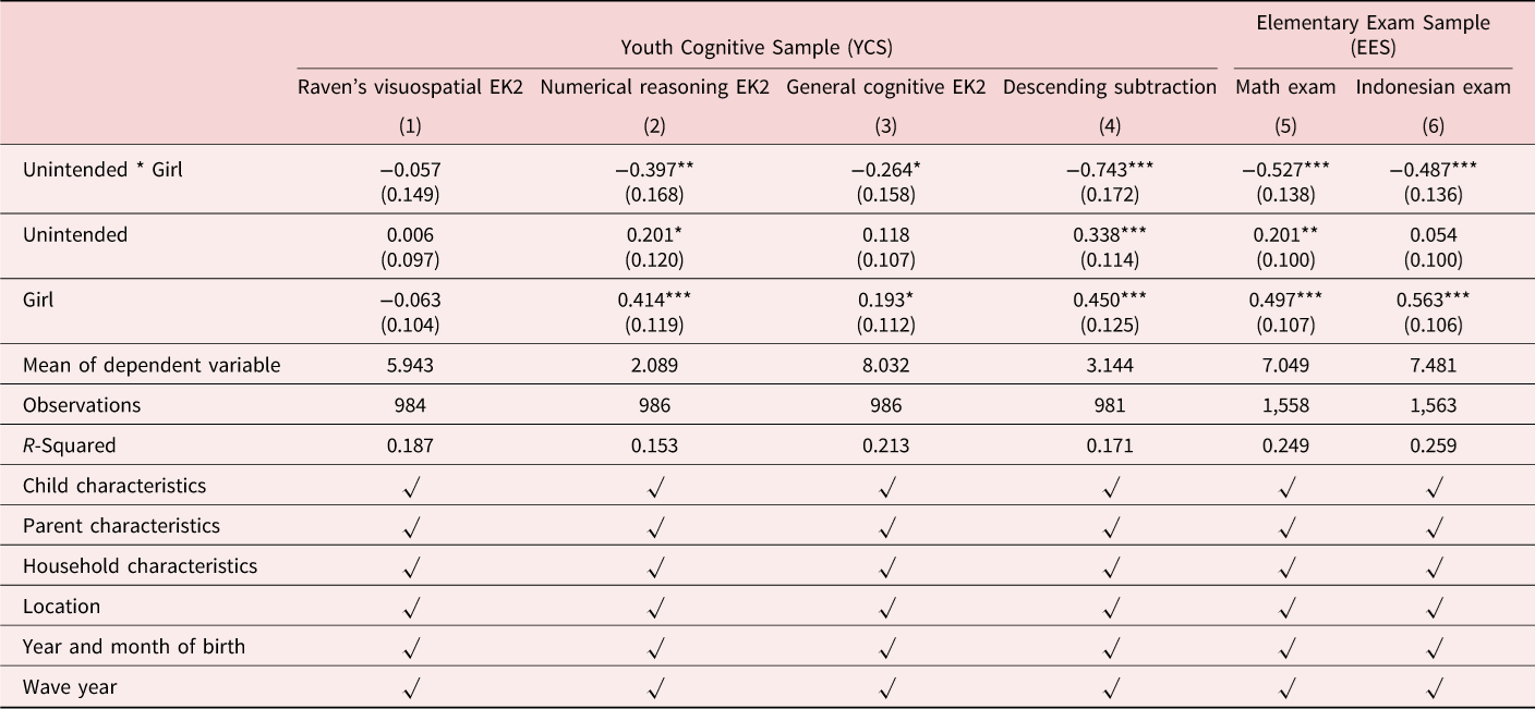
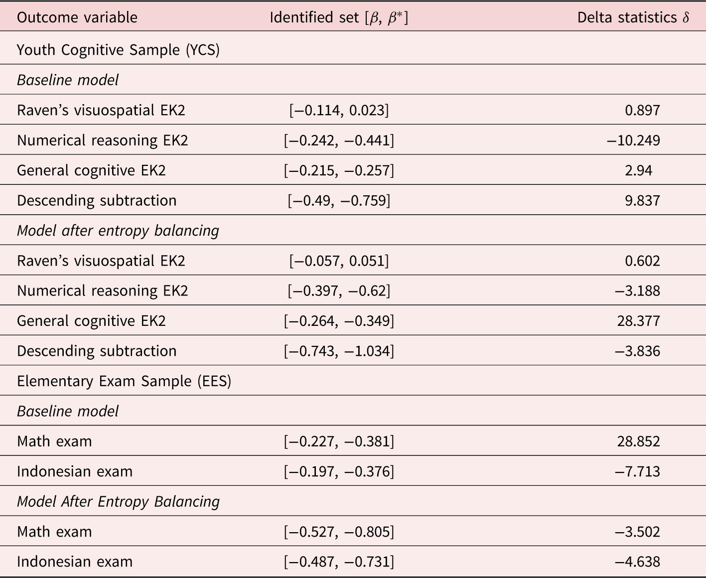


 Open access

