1. Introduction
The buoyancy-driven flow of a fluid heated from below and cooled from above, Rayleigh–Bénard convection, is a classical prototype for many applications of industrial or meteorological interest. One intriguing fact is the existence of a large-scale circulation in the turbulent regime at high Rayleigh numbers (Krishnamurti & Howard Reference Krishnamurti and Howard1981). The circulation depends on the aspect ratio of the domain and varies in time (see, for instance, Xi & Xia Reference Xi and Xia2008). These variations, or reversals, preserve the statistical symmetries of the flow. Such flow reversals appear in a variety of situations, ranging from magnetohydrodynamics to weather systems.
Reorganization of the large-scale circulation in a cylindrical cell has been studied in detail (see, for instance, Niemela et al. Reference Niemela, Skrkbek, Streenivasan and Donelly2001; Brown & Ahlers Reference Brown and Ahlers2007; Benzi & Verzicco Reference Benzi and Verzicco2008). Cessation as well as rotation were identified as two different mechanisms associated with strong variations of the large-scale circulation (Brown, Nikolaenko & Ahlers Reference Brown, Nikolaenko and Ahlers2005). Considerable effort has been spent in putting together models to reproduce the flow behaviour. Statistical models have been proposed by Sreenivasan, Berdshadskii & Niemelak (Reference Sreenivasan, Berdshadskii and Niemelak2002), Araujo, Grossmann & Lohse (Reference Araujo, Grossmann and Lohse2005), Benzi (Reference Benzi2005) and Brown & Ahlers (Reference Brown and Ahlers2007). Sreenivasan et al. (Reference Sreenivasan, Berdshadskii and Niemelak2002) argued that the generation of the large-scale circulation and its reversal was the result of an imbalance between buoyancy and viscous effects. Araujo et al. (Reference Araujo, Grossmann and Lohse2005) computed the force and thermal balance on a single plume to explain the dynamics of the flow using a water-wheel analogy. Benzi (Reference Benzi2005) showed that the dynamics of reversals could be represented with a system of stochastic differential equations even in the absence of a time scale separation between the large-scale circulation and the turbulent fluctuations. Based on physical arguments, Brown & Ahlers (Reference Brown and Ahlers2007) derived a system of two stochastic equations to describe the evolution of the strength and the azimuthal orientation of the large-scale circulation. Their model reproduces both rotations and cessations.
The influence of small scales on the evolution of the large scales appears to be an essential ingredient of turbulent natural convection. However, it is not clear whether noise is an essential part of the reversal process or whether reversals are a consequence of deterministic chaos. Gallet et al. (Reference Gallet, Hérault, Laroche, Pétrélis and Fauve2012) showed that reversals of a large-scale field generated by a turbulent background could occur in a deterministic dynamical systems as a consequence of symmetry restoring.
The situation may be simpler to examine in a 2D or nearly 2D cell rather than in a cylindrical cell, as rotation effects are then eliminated and the circulation simply switches signs. Such reversals of the large-scale organization of 2D turbulence in a square cell (without convection) have been numerically observed by Molenaar, Clercx & van Heijst (Reference Molenaar, Clercx and van Heijst2004) and found to be connected to the development of vortex filaments along the viscous walls. The characteristics of flow reversals in 2D or quasi-2D Rayleigh–Bénard cells have been studied by Sugiyama et al. (Reference Sugiyama, Ni, Stevens, Chan, Zhou, Xi, Sun, Grossmann, Xia and Lohse2010) in a square cell, both numerically and experimentally, as well as Chandra & Verma (Reference Chandra and Verma2011) and Petschel et al. (Reference Petschel, Wilczek, Breuer, Fredrich and Hansen2011). Sugiyama et al. (Reference Sugiyama, Ni, Stevens, Chan, Zhou, Xi, Sun, Grossmann, Xia and Lohse2010) identified a confined range of Rayleigh and Prandtl numbers for which reversals occur, and showed how the existence of reversals depended on these parameters. They proposed that reversals depend on the growth of corner flows, which requires the Prandtl number to be small enough to allow thermal coupling, yet to remain large enough so that the motion will not be entirely damped by thermal dissipation effects.
Chandra & Verma (Reference Chandra and Verma2011) used Fourier analysis to study reversals in a 2D Rayleigh–Bénard cell. They identified a
 $(1,1)$
mode and a
 $(2,2)$
mode, which correspond to respectively one (large-scale circulation) and four convection rolls (quadrupolar flow). They found that the existence of this last mode was a necessary condition for the existence of reversals. More recently, Chandra & Verma (Reference Chandra and Verma2013) showed that reversals occurred through vortex reconnection of two attracting corner rolls having the same vorticity.
In this paper we also consider the 2D direct numerical simulation (DNS) of Rayleigh–Bénard convection in a square cell. We use POD analysis to extract the coherent structures associated with the flow. POD-based models for chaotic natural convection were first derived more than two decades ago by Sirovich & Park (Reference Sirovich and Park1990), Deane & Sirovich (Reference Deane and Sirovich1991) and Lumley & Poje (Reference Lumley and Poje1997). Recent applications include Bailon-Cuba, Emran & Schumacher’s (Reference Bailon-Cuba, Emran and Schumacher2010) work, where a POD-based model was derived to represent the flow at a Rayleigh number of
 $10^{5}$
, and Podvin & Sergent (Reference Podvin and Sergent2012), in which POD was applied to turbulent Rayleigh–Bénard convection in a 3D rectangular box to reproduce the large-scale reversal dynamics of convection rolls.
The advantages of the POD approach are that modes are generated directly from the data without assumptions and account for boundary conditions in an organic manner. Moreover, coupling between different physical quantities such as the velocity and temperature appears naturally, as will be detailed below. The goals of the paper are: (i) to provide a detailed description of the physical processes at work in reversals of the large-scale circulation; (ii) to attempt to reproduce the dynamics of reversal with a low-order model. In contrast with the approaches mentioned above where specific flow features are selected and modelled, the model is obtained from a Galerkin projection of the Navier–Stokes equations onto the basis of empirical POD eigenfunctions. This means that extensive information about second-order statistics is necessary to obtain the eigenfunctions from which the coefficients of the model are computed. Furthermore, additional closure assumptions need to be made if only a few modes are retained, which is the case here.
The paper is organized as follows: we first present the numerical simulation, the results of which are analysed with POD. We then show that the reversal mechanism can be captured with a three-dimensional model in the presence of noise.
2. The configuration
2.1. The equations of motion
We consider a square domain filled with water (
 $\mathit{Pr}={\it\nu}/{\it\kappa}=4.3$
) heated at the bottom and cooled at the top. The flow regime depends on the Rayleigh number
 $$\begin{eqnarray}\mathit{Ra}=\frac{\tilde{{\it\alpha}}g{\rm\Delta}Th^{3}}{{\it\nu}{\it\kappa}}\end{eqnarray}$$
where
 $\tilde{{\it\alpha}}$
is the volumetric thermal expansion coefficient,
 $g$
is gravity,
 ${\rm\Delta}T$
is the temperature difference between both isothermal horizontal plates,
 $h$
is the height between the horizontal plates and
 ${\it\nu}$
and
 ${\it\kappa}$
are the fluid kinematic viscosity and thermal diffusivity, respectively. The Rayleigh number is set to
 $\mathit{Ra}=5\times 10^{7}$
, which corresponds to a flow regime where intermittency is expected, according to figure 4 from Sugiyama et al. (Reference Sugiyama, Ni, Stevens, Chan, Zhou, Xi, Sun, Grossmann, Xia and Lohse2010). Computations were also run at
 $\mathit{Ra}=10^{8}$
. However, results were found to be quite similar and we only show results for the case
 $\mathit{Ra}=5\times 10^{7}$
.
The flow equations are based on the Boussinesq approximation. The reference length and velocity units used to make the equations non-dimensional are the height between the plates
 $h$
and the velocity
 $({\it\kappa}/h)\sqrt{\mathit{Ra}}$
. The temperature is made dimensionless with
 ${\rm\Delta}T$
. The horizontal and vertical directions will respectively be labelled
 $x$
and
 $z$
. If
 $\boldsymbol{u}$
is the velocity vector (
 $\boldsymbol{u}=(u,w)$
) and
 ${\it\theta}$
the dimensionless temperature, then the equations based on the non-dimensional reference units are
 $$\begin{eqnarray}\displaystyle & \boldsymbol{{\rm\nabla}}\boldsymbol{\cdot }\boldsymbol{u}=0 & \displaystyle\end{eqnarray}$$
 $$\begin{eqnarray}\displaystyle & \displaystyle \frac{\partial u}{\partial t}+u\frac{\partial u}{\partial x}+w\frac{\partial u}{\partial z}=-\frac{\partial p}{\partial x}+\frac{\mathit{Pr}}{\mathit{Ra}^{1/2}}{\rm\Delta}u & \displaystyle\end{eqnarray}$$
 $$\begin{eqnarray}\displaystyle & \displaystyle \frac{\partial w}{\partial t}+u\frac{\partial w}{\partial x}+w\frac{\partial w}{\partial z}=-\frac{\partial p}{\partial z}+\frac{\mathit{Pr}}{\mathit{Ra}^{1/2}}{\rm\Delta}w+\mathit{Pr}{\it\theta} & \displaystyle\end{eqnarray}$$
 $$\begin{eqnarray}\displaystyle & \displaystyle \frac{\partial {\it\theta}}{\partial t}+u\frac{\partial {\it\theta}}{\partial x}+w\frac{\partial {\it\theta}}{\partial z}=\frac{1}{\mathit{Ra}^{1/2}}{\rm\Delta}{\it\theta}. & \displaystyle\end{eqnarray}$$
The velocity is zero on all walls. The temperature is set to 0.5 and
 $-$
0.5 on the bottom and top wall, respectively. Adiabatic conditions are used on the side walls.
If we consider the origin of the axes
 $(x^{\ast },z^{\ast })$
to be set in the centre of the cell, the symmetries of the problem are as follows:
-
(i) the reflexion symmetry
 $S_{x}$
with respect to the vertical axis
$x^{\ast }=0$
which leaves all physical quantities invariant (2.6)
$$\begin{eqnarray}\left[\begin{array}{@{}c@{}}u\\ w\\ {\it\theta}\end{array}\right](x^{\ast },z^{\ast })\rightarrow \left[\begin{array}{@{}c@{}}-u\\ w\\ {\it\theta}\end{array}\right](-x^{\ast },z^{\ast })\end{eqnarray}$$
-
(ii) the reflexion symmetry
$S_{z}$
with respect to the horizontal axis
$z^{\ast }=0$
which leaves the velocity invariant and transforms the temperature variation into its opposite (2.7)
$$\begin{eqnarray}\left[\begin{array}{@{}c@{}}u\\ w\\ {\it\theta}\end{array}\right](x^{\ast },z^{\ast })\rightarrow \left[\begin{array}{@{}c@{}}u\\ -w\\ -{\it\theta}\end{array}\right](x^{\ast },-z^{\ast });\end{eqnarray}$$
-
(iii) the rotation of origin the cell centre
$(x^{\ast },z^{\ast })=(0,0)R_{{\it\pi}}=S_{x}\circ S_{z}=S_{z}\circ S_{x}$
(2.8)
$$\begin{eqnarray}\left[\begin{array}{@{}c@{}}u\\ w\\ {\it\theta}\end{array}\right](x^{\ast },z^{\ast })\rightarrow \left[\begin{array}{@{}c@{}}-u\\ -w\\ -{\it\theta}\end{array}\right](-x^{\ast },-z^{\ast }).\end{eqnarray}$$




Along with the identity, this forms a four-dimensional symmetry group.
2.2. The numerical method
The simulations are carried out with a multidomain spectral code, which is based on a time marching procedure and a spectral collocation method for spatial discretization. Time integration of the governing equations (1)–(4) is performed through a second-order semi-implicit scheme. It combines a second-order backward Euler scheme with an implicit treatment for the diffusion terms and an explicit second-order Adams–Bashforth extrapolation for the nonlinear terms. Incompressibility is imposed by a projection method which retains second-order accuracy of the time integration. The domain decomposition in the horizontal direction
 $x$
is carried out by the Schur complement method and implemented with the MPI library. Chebyshev modes are used in all directions. Details of the method can be found in Xin, Chergui & Le Quéré (Reference Xin, Chergui and Le Quéré2008).
Time integration of the governing equations is started from a lower Rayleigh number solution and is carried out long enough for the flow regime to become statistically established. The present simulation has been performed with a Chebyshev spectral collocation approximation using 384 points or polynomials in the horizontal direction, 158 points in the vertical direction. The time step is equal to 0.0006 convective time units.
The spatial accuracy of the present results has been checked by looking at the decay of the spectral coefficients of the temperature or velocity fields. A close inspection of these coefficients shows that they decrease with increasing order, and a ratio larger than
 $10^{5}$
is consistently observed between the smallest and the largest modes.
2.3. 2D reversal sequence: flow description
The physical configuration meets the conditions for reversal determined by Sugiyama et al. (Reference Sugiyama, Ni, Stevens, Chan, Zhou, Xi, Sun, Grossmann, Xia and Lohse2010). The present results cover more than 37 500 convective time units (which corresponds to around 15 days of measurement in a 20 cm cell at
 $40\,^{\circ }\text{C}$
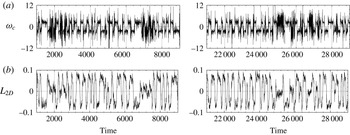
). Figure 1 shows the time evolution of standard indicators of reversals such as the vorticity
 ${\it\omega}_{c}$
at the centre of the cavity and the global angular momentum
 $L_{2D}$
defined as
 $L_{2D}(t)=\int _{V}\boldsymbol{u}\times \underline{x}^{\ast }\,\text{d}V$
. The sign of the vorticity and of the global angular momentum remains nearly constant for some periods of time, then experiences a rapid switch. This switch between two well-defined states is associated with what we will call throughout the paper a standard reversal. This classical process of reversal by corner roll growth has been described previously by Sugiyama et al. (Reference Sugiyama, Ni, Stevens, Chan, Zhou, Xi, Sun, Grossmann, Xia and Lohse2010), Chandra & Verma (Reference Chandra and Verma2013).
(a) Time evolution of the vorticity at the cell centre
 ${\it\omega}_{c}$
. (b) Evolution of the angular momentum
 $L_{2D}$
(see the definition in the text).

We will define the large eddy turnover time as
 ${\it\tau}_{E}=4{\rm\pi}/\langle |{\it\omega}_{c}(t)|\rangle$
(here
 ${\it\tau}_{E}=4.9$
convective time units). Two different large-scale flow patterns stable over more than 10
 ${\it\tau}_{E}$
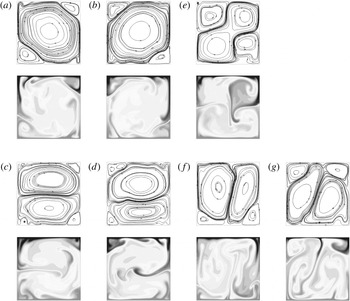
are observed in the simulation. They are plotted in figure 2. It should be mentioned that the time series is long enough to collect converged lifetime statistics for some large-scale modes. As expected, one of the stable patterns (and its image through
 $S_{x}$
or
 $S_{z}$
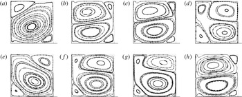
) corresponds to a diagonal large-scale roll along with two smaller counter-rotative rolls located in the opposite corners is found. The transition between the diagonal rolls involves a transitory quadrupolar flow pattern (see figure 2
e) associated with the growth of the corner rolls.
Typical large-scale flow patterns: streamlines and temperature isocontours of instantaneous fields. (a–d) Stable large-scale flow structures observed for more than
 $10{\it\tau}_{E}$
: (a)
 $t=2900$
; (b)
 $t=3014$
; (c)
 $t=2627$
; (d)
 $t=1955$
. (e–g) Transient large-scale patterns connecting stable large-scale flow structures: (e)
 $t=2954$
; (f)
 $t=2801$
; (g)
 $t=2309$
.

The second type of ‘quasi-stable’ large-scale flow pattern (and its image through
 $S_{x}$
) consists of two counter-rotative, horizontally stacked rolls. Smaller corner rolls are located at the ends of the vertical wall where the flow is diverging. This second flow pattern has been found to be dominant by Chandra & Verma (Reference Chandra and Verma2013) in a small range of
 $\mathit{Ra}$
(
 $\mathit{Ra}=10^{6}{-}10^{7}$
at
 $\mathit{Pr}=1$
) before the reversal regime, and has been observed as a transient by Xi & Xia (Reference Xi and Xia2008) in a water-filled cylinder of aspect ratio 1 at
 $\mathit{Ra}\approx 10^{9}$
. This flow pattern is associated with transient structures corresponding to two vertically stacked rolls (figure 2
f,g) resulting from a
 ${\rm\pi}/2$
rotation of the dominant modes. This rotation phenomenon has also been previously observed by Chandra & Verma (Reference Chandra and Verma2013).
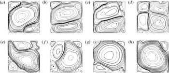
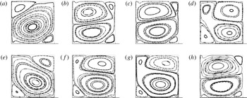
Consequently, two types of transition mechanisms can be identified in the time series: (i) the growth of the corner rolls leading to the transient observation of the quadrupolar flow; and (ii) the rotation of the large-scale pattern (either the diagonal roll or the two stacked rolls). In most cases a complete or standard reversal involves the two mechanisms, as seen by Sugiyama et al. (Reference Sugiyama, Ni, Stevens, Chan, Zhou, Xi, Sun, Grossmann, Xia and Lohse2010) or Chandra & Verma (Reference Chandra and Verma2011). Such a reversal is illustrated in figure 3. It is achieved by corner roll growth (figure 3
b,c) followed by the brief appearance of the quadrupolar flow (figure 3
d), then rotation (figure 3
e–g) leading to a large-scale diagonal roll pattern opposed to the initial one (figure 3
h). It corresponds to the fast and direct sign switch in the
 $L_{2D}$
time series as seen in figure 1.
Flow streamlines of selected snapshots during a standard reversal: (a)
 $t=3428$
; (b)
 $t=3449$
; (c)
 $t=3452$
; (d)
 $t=3455$
; (e)
 $t=3458$
; ( f)
 $t=3461$
; (g)
 $t=3467$
; (h)
 $t=3476$
.

In other instances, as can be seen in figure 1 at
 $t\approx 1800$
,
 $t\approx 2300$
or
 $t\approx 5000$
, the reversal process appears to be more complicated. It is characterized by rapid, erratic oscillations of
 ${\it\omega}_{c}$
and a value of
 $L_{2D}$
close to 0. For this reason, we will refer to these events as cessations, as it seems that the single large-scale circulation no longer seems well-defined at these times. They correspond to a succession of corner roll growth and/or rotation events, which ends with the recovery of a stable diagonal roll pattern. In most cases, the final roll pattern keeps the orientation of the initial one, as for example in the sequence around
 $t\approx 2300$
or
 $t\approx 5000$
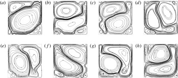
. This phenomenon was previously observed by Xi & Xia (Reference Xi and Xia2008) in a cylinder and Sugiyama et al. (Reference Sugiyama, Ni, Stevens, Chan, Zhou, Xi, Sun, Grossmann, Xia and Lohse2010) in a square cell. Figure 4 illustrates a portion of this reversal process. The diagonal roll splits into two horizontally stacked rolls (figure 4
b), which then rotate around the cell (figure 4
d–h).
Flow streamlines of selected snapshots during a cessation: (a)
 $t=1718$
; (b)
 $t=1742$
; (c)
 $t=1748$
; (d)
 $t=1754$
; (e)
 $t=1760$
. ( f)
 $t=1766$
; (g)
 $t=1769$
; (h)
 $t=1772$
.

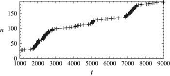
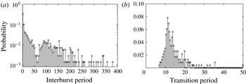
We note that these erratic transitions are more rarely observed in the simulation. In the complete time series, around 75 cessations are observed. Cessations can be clearly identified in figure 5, where sign switches of
 $L_{2D}$
are recorded. To distinguish cessations from standard reversals, we observe on figure 5 that a cessation produces fast
 $L_{2D}$
switches with a characteristic time scale. This time scale can be deduced from figure 6(a), where the probability density function (PDF) of the time intervals
 ${\it\tau}_{1}$
between two successive sign switches of
 $L_{2D}$
is plotted. A time cut-off criterion between fast and slow switches can be established at around
 ${\it\tau}_{c}=12{\it\tau}_{E}$
(63 convective time units): a cessation produces fast
 $L_{2D}$
switches with a characteristic time scale of less than
 ${\it\tau}_{c}$
, whereas the characteristic time scale of standard reversals is greater than
 ${\it\tau}_{c}$
. The sequences of rapid switches happen at time intervals of the order of
 $200{\it\tau}_{E}$
and can last up to
 $50{\it\tau}_{E}$
.
Occurrence of reversals: a symbol (
 $+$
) is plotted when
 $L_{2D}=0$
. Here
 $n$
corresponds to the number of crossings of the
 $y$
-axis.

(a) PDF of time intervals
 ${\it\tau}_{1}$
between successive instances of
 $L_{2D}=0$
. (b) PDF of the transition duration
 ${\it\tau}_{d}$
during a standard reversal defined as the time during which
 $|L_{2D}|<0.3L_{max}$
.

In contrast, in the present time series, approximately 230 standard reversals were observed. The mean duration of a standard reversal is approximately
 $2{\it\tau}_{E}$
(11 convective time units), as can be seen in the PDF of the transition duration (figure 6
b). The mean time between successive standard reversals
 ${\it\tau}_{1}$
is found to be equal to
 $\langle {\it\tau}_{1}\rangle =29.6{\it\tau}_{E}|_{({\it\tau}_{1}\geqslant 12{\it\tau}_{E})}$
(approximately 145 convective time units). This is in good agreement with the findings of Sugiyama et al. (Reference Sugiyama, Ni, Stevens, Chan, Zhou, Xi, Sun, Grossmann, Xia and Lohse2010).
The idea is now to use POD to investigate in detail the reversal dynamics.
3. POD analysis of the flow
Due to the size of the physical grid,
 $O(50\,000)$
, the method of snapshots (Sirovich Reference Sirovich1987) was used to extract empirical eigenfunctions. POD analysis was applied to 750 snapshots separated by six reference time units for the case
 $\mathit{Ra}=5\times 10^{7}$
. Flow symmetries were not used to increase the size of the snapshot ensemble, so as to preserve the particular symmetry of the simulation. Using snapshots collected over a shorter time length spanning only a few reversals and/or with a shorter sampling time did not affect the results, which gives us some confidence in the robustness of our observations.
The basic idea of POD (Holmes, Lumley & Berkooz Reference Holmes, Lumley and Berkooz1996) is that physical quantities characterizing the flow such as the velocity
 $\boldsymbol{u}$
or temperature
 ${\it\theta}$
can be written as a superposition of spatial structures or empirical eigenfunctions
 $\underline{{\it\phi}}(\underline{x})$
. These functions are orthogonal and their amplitudes
 $a^{n}(t)$
, vary in time. One has
 $$\begin{eqnarray}\underline{q}(\underline{x},t)=\mathop{\sum }_{n=1}^{\infty }a^{n}(t)\underline{{\it\phi}}_{\underline{q}}(\underline{x}).\end{eqnarray}$$
The POD modes are hierarchically organized according to their energy
 ${\it\lambda}_{n}$
. If the empirical eigenfunctions are normalized, we have
 $\langle a^{n}(t)a^{m}(t)\rangle ={\it\delta}_{nm}{\it\lambda}_{n}$
where
 ${\it\delta}_{nm}$
is the Kronecker symbol and
 $\langle \,\rangle$
is a time average. For more details see Holmes et al. (Reference Holmes, Lumley and Berkooz1996).
A classical question when applying POD to thermal convection flows is whether to treat the velocity and the temperature separately or jointly. In the latter case, the introduction of an arbitrary rescaling factor is inevitable since they correspond to different physical quantities. Lumley & Poje (Reference Lumley and Poje1997) argued that using a joint formulation allowed POD to capture the velocity/temperature coupling. This argument was also used by Podvin & Le Quéré (Reference Podvin and Le Quéré2001) and Bailon-Cuba et al. (Reference Bailon-Cuba, Emran and Schumacher2010). In contrast Jing et al. (Reference Jing, Henry, Hadid and Imaishi2003) found that separate expansions for the velocity and temperature led to better approximations in low-dimensional models.
To carry out the POD of a set of variables
 $\underline{q}$
, one solves the following eigenvalue problem:
 $$\begin{eqnarray}\langle \underline{q}(\underline{x},t)\underline{q}(\underline{x}^{\prime },t)\rangle \underline{{\it\phi}}_{\underline{q}}(\underline{x}^{\prime })\,\text{d}\underline{x}^{\prime }={\it\lambda}\underline{{\it\phi}}_{\underline{q}}(\underline{x})\end{eqnarray}$$
where
 $\langle \underline{q}(\underline{x},t)\underline{q}(\underline{x}^{\prime },t)\rangle$
is the spatial autocorrelation tensor. The spatial autocorrelation tensor is usually computed from
 $N$
individual snapshots obtained at instants
 $t^{n}$
,
 $\underline{q}(\underline{x},t^{n})$
:
 $$\begin{eqnarray}\langle \underline{q}(\underline{x},t)\underline{q}(\underline{x}^{\prime },t)\rangle =\frac{1}{N}\mathop{\sum }_{n=1}^{N}\underline{q}(\underline{x},t^{n})\underline{q}(\underline{x}^{\prime },t^{n}).\end{eqnarray}$$
In the method of snapshots (Sirovich Reference Sirovich1987), we use the fact that the eigenfunctions can be written as the linear combination of these
 $N$
snapshots
 $$\begin{eqnarray}\underline{{\it\phi}}_{\underline{q}}(\underline{x})=A^{p}\underline{q}(\underline{x},t^{p})\end{eqnarray}$$
to rewrite the eigenvalue problem. One can show that
 $A^{p}$
represents the temporal amplitude of the mode
 $\underline{{\it\phi}}^{n}$
at time
 $t^{p}$
, i.e.
 $$\begin{eqnarray}A^{p}=a^{n}(t^{p}).\end{eqnarray}$$
If the decomposition is applied to some variables
 $\underline{q}$
, for instance the velocity or the temperature field, extended spatial eigenfunctions for different variables
 $\underline{r}$
can be obtained by applying the above expansion:
 $$\begin{eqnarray}\underline{{\it\phi}}_{\underline{r}}(\underline{x})=A^{p}\underline{r}(\underline{x},t^{p}).\end{eqnarray}$$
This procedure constitutes extended POD (see Boree (Reference Boree2003)). It is therefore possible to educe temperature functions from a velocity-based decomposition and vice versa. The method of snapshots can thus provide a coupled expansion for the thermal and velocity eigenfunctions, independently from the variables used to perform the POD.
Three different formulations were considered and compared a velocity-based, a temperature-based and a joint velocity/temperature formulation (mixed formulation). We therefore solved the following eigenvalue problem
 $$\begin{eqnarray}C{\it\Phi}={\it\lambda}{\it\Phi}\end{eqnarray}$$
for three different expressions of
 $C$
, as follows.
-
(i) The velocity-based formulation:
(3.8)
$$\begin{eqnarray}C_{\boldsymbol{u}}^{nm}=\frac{1}{N}\int \boldsymbol{u}(\underline{x},t^{n})\boldsymbol{\cdot }\boldsymbol{u}(\underline{x},t^{m})\,\text{d}\underline{x}.\end{eqnarray}$$
-
(ii) The temperature-based formulation:
(3.9)
$$\begin{eqnarray}C_{{\it\theta}}^{nm}=\frac{1}{N}\int {\it\theta}(\underline{x},t^{n}){\it\theta}(\underline{x},t^{m})\,\text{d}\underline{x}.\end{eqnarray}$$
-
(iii) The mixed formulation:
(3.10)Here the rescaling factor for the temperature relative to the velocity was set to 1.
$$\begin{eqnarray}C_{full}^{nm}=\frac{1}{N}\int (\boldsymbol{u}(\underline{x},t^{n})\boldsymbol{\cdot }\boldsymbol{u}(\underline{x},t^{m})+{\it\theta}(\underline{x},t^{n}){\it\theta}(\underline{x},t^{m}))\,\text{d}\underline{x}.\end{eqnarray}$$


3.1. Physical modes
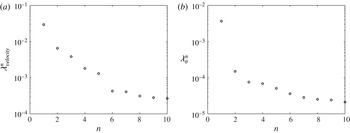
The first five modes in the velocity and temperature decomposition capture 90 % and 80 % of the respective kinetic and thermal energy (defined as respectively
 $\Vert \boldsymbol{u}\Vert ^{2}$
and
 ${\it\theta}^{2}$
). The first three modes capture respectively 83 % and 76 % of the energy. The corresponding POD spectra are shown in figure 7 for the first 10 modes.
POD spectrum: (a) velocity formulation; (b) temperature formulation.

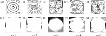
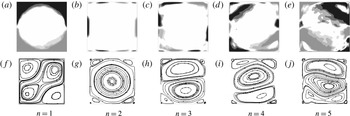
Figures 8 and 9 shows the POD empirical velocity (respectively temperature) eigenfunctions and the extended temperature (respectively velocity) modes for the velocity-based (respectively temperature-based) formulation. In all figures from now on, unless mentioned otherwise, the origin of the axes will be set at the bottom left corner of the cell. We note some similarity between the first most energetic modes. Specifically, the most energetic velocity-based mode (
 $n=1$
in figure 8) consists of a large circulation cell, with some recirculations in the corner and similar to the mode
 $(1,1)$
of Chandra and Verma. The velocity updraft along one of the vertical walls corresponds to a positive temperature fluctuation, while the downdraft along the opposite wall corresponds to a negative one. This mode (both velocity and temperature) is similar to the second mode obtained with the temperature-based POD formulation. The mode is antisymmetric with respect to both
 $S_{x}$
and
 $S_{z}$
symmetry, i.e.
 $S\underline{{\it\phi}}=-\underline{{\it\phi}}$
for
 $S\in \{S_{x},S_{z}\}$
. This means that
 $R_{{\it\pi}}\underline{{\it\phi}}=\underline{{\it\phi}}$
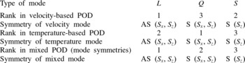
. This mode is also similar to the most energetic mode in the mixed velocity temperature formulation with a rescaling factor of 1. Since different formulations lead to different orderings, we will avoid to use indices to refer to POD modes and will call this mode the large-scale circulation (
 $L$
).
Velocity-based formulation: (a–e) POD velocity modes; ( f–j) educed temperature modes (isothermals range from
 $-$
0.2 to 0.2 with an increment of 0.05).

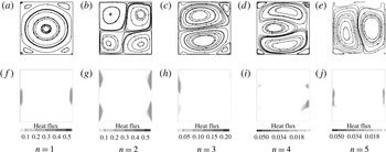
Temperature-based formulation: (a–e) POD temperature modes (isothermals range from
 $-$
0.2 to 0.2 with an increment of 0.05); ( f–j) educed velocity modes.

The most energetic temperature-based mode contains the mean temperature (
 $n=1$
, in figure 9
a–e), which is associated with a quadrupolar flow bringing fluid into the centre of the cell (
 $n=1$
, in figure 9
f–j). It corresponds to mode
 $(2,2)$
in Chandra & Verma’s (Reference Chandra and Verma2011) analysis. This mode is entirely symmetric, i.e.
 $S\underline{{\it\phi}}=\underline{{\it\phi}}$
for
 $S\in \{S_{x},S_{z},R_{{\it\pi}}\}$
. Note that due to the presence of vertical walls, changing the sign of the circulations would correspond to a different physical mode (see also the next section). This mode appears in the velocity decomposition as the third most energetic mode (
 $n=3$
in figure 8). We will refer to this mode as the quadrupolar mode (
 $Q$
).
The second most energetic mode in the velocity-based formulation consists of two cells superposed in the vertical direction (
 $n=2$
, in figure 8
a–e). It satisfies the
 $S_{z}$
horizontal reflexion symmetry, but it does not seem to satisfy the
 $R_{{\it\pi}}$
or the
 $S_{x}$
symmetry, as is apparent from the representation of temperature (
 $n=2$
, in figure 8
f–j). One way to understand this lack of symmetry is to realize that at one horizontal end of the cell, fluid comes in from the hot and cold regions and is therefore associated with stronger temperature gradients than that leaving the core region at the other end of the cell. This symmetry-breaking, double-roll mode also corresponds to the third most energetic mode in the velocity-based formulation and will be referred to as the
 $S$
mode (for symmetry-breaking).
The fourth velocity mode consists of two corotating vortices at the bottom and the top of the cavity, with another counter-rotating vortex tucked in between the two. The corresponding temperature mode appears to be antisymmetric with respect to the vertical reflection symmetry. The fifth velocity mode consists of two tall cells extending over one half-width and the full height of the cavity. It corresponds to the seventh most energetic mode (not shown) in the temperature decomposition. The sixth velocity mode (not shown) appears to be a combination of the large cell (mode 1) and the quadrupolar cell (mode 2), and therefore can be considered to be the result of nonlinear interactions between these modes.
In the temperature-based decomposition the temperature modes 4 and 5 in figure 9( f–j) appear to be symmetric from each other, which is confirmed by examination of the corresponding educed velocity modes in figure 9(a–e). They correspond to three rolls of uneven sizes extending over the width of the cell. The educed velocity modes appear to satisfy the vertical symmetry
 $S_{x}$
, but again this is not satisfied by the temperature modes. Despite differences between the velocity-based and the temperature-based POD formulation, higher-order modes
 $\underline{{\it\phi}}^{n}$
with
 $n>3$
essentially consist of horizontally stacked, symmetry-breaking rolls.
Velocity modes in the mixed formulation are shown in figure 10 and appear to be similar to the velocity formulation, allowing for some reordering (the
 $Q$
mode becomes the second most important). Representation of the heat flux associated with the different modes in the mixed formulation in figure 10 shows that the contributions of the large-scale circulation and the quadrupolar mode are dominant and correspond to heat transfer occurring along the vertical boundaries. The contribution of the
 $L$
mode is predominant in the centre section of the vertical boundary layers, while that of the
 $Q$
mode is concentrated in the corners of the cells. The large-scale circulation therefore plays a crucial role in transferring heat from the bottom to the top horizontal boundary layers.
Mixed formulation: (a–e) POD velocity modes; ( f–j) contribution to the convective heat flux
 ${\it\phi}_{w}^{n}{\it\phi}_{{\it\theta}}^{n}{\it\lambda}^{n}$
.

To sum up, both velocity and temperature-based decompositions point to the emergence of the following modes: an antisymmetric large-scale circulation, a symmetric mean temperature mode associated with a quadrupolar flow, a symmetry-breaking, double-roll mode, and a set of symmetry-breaking roll modes satisfying only partially flow symmetries. The symmetries associated with the first three modes corresponding to the different POD formulations are summarized in table 1.
Hierarchy of modes according to the POD formulation and corresponding symmetry (S) or antisymmetry (AS).

3.2. Temporal amplitudes
3.2.1. Long-term behaviour
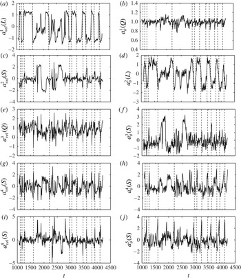
Figure 11 shows the evolution of the amplitudes of the first POD velocity and temperature modes during a large number of reversals. It confirms that two different kinds of excursions can occur. In the standard reversal (most frequent case), the large-scale circulation (figure 11
a, left column, and figure 11
b, right column) switches between two nearly constant values. In between reversals of the large-scale circulation, the amplitude of the mode
 $L$
evolves on a much slower time scale than during reversals. In the cessation case, the large-scale circulation is close to zero (for example, around
 $t\approx 1800{-}2000$
). In general, we note that the temperature mode
 $L$
(figure 11
b, right column) seems to experience smoother transitions than the velocity mode
 $L$
(it is more like a sine wave than a step function), so that reversals can be first detected in the temperature mode.
History of the velocity modes (left) and the temperature modes (right): (a)
 $n=1$
, (b)
 $n=2$
, (c)
 $n=3$
, (d)
 $n=4$
, (e)
 $n=5$
; dashed lines are used to identify selected reversals.

In both formulations, the amplitude of the quadrupolar mode
 $Q$
(figure 11
c, left column, and figure 11
a, right column), which corresponds to mode
 $(2,2)$
in Chandra & Verma (Reference Chandra and Verma2013), fluctuates near a positive value. At the onset of standard reversals it slightly increases then strongly decreases and can even change sign during reversal in the case of the velocity mode. We note that changing the sign of the second mode
 $(u,w,{\it\theta})(x,z)\rightarrow (-u,-w,-{\it\theta})(x,z)$
does not correspond to a physical symmetry of the system, on account of the lateral rigid walls along which heat flux takes place (figure 10): for heat transfer to be efficient, the flow needs to move away from the horizontal boundaries along the vertical walls. This explains why the sign of the amplitude of the second mode remains nearly constant except during brief intervals following reversals. The fluctuations of the temperature mode
 $Q$
are less significant as it is associated with the mean temperature. Moreover, in the case of the cessation (see
 $t\approx 1800$
and 2500), the velocity mode (figure 11
c, left) collapses while the temperature mode (figure 11
a, right) is slightly strengthened.
The double-roll, symmetry-breaking mode (figure 11
b, left column, and figure 11
c, right column) experiences sharp fluctuations during standard reversals. It is otherwise small when the large-scale single-roll mode
 $L$
is established. In the case of cessations, it takes a nearly constant high value.
Figure 11(d,e) confirm that during standard reversals, all higher-order modes
 $n\geqslant 4$
are characterized by violent, both positive and negative excursions, thereby indicating a significant change in the physical structure of the flow. However, the skewness of the temporal amplitudes is in general different from zero: this lack of symmetry corresponds to the symmetry-breaking observed in the physical space. During cessations, the higher-order modes also settle near relatively high, constant values.
3.2.2. Flow reconstruction during reversals
We now consider low-dimensional projections of the flow onto the first POD modes. We will use the modes obtained with the mixed formulation. Figures 12 and 13 show snapshots of the projection of the flow onto the first three modes (capturing more than 80 % of the POD energy) for the two types of flow excursions illustrated in figures 3 and 4.
Snapshots from figure 3 projected on the first three mixed velocity modes (standard reversal): (a)
 $t=3428$
; (b)
 $t=3449$
; (c)
 $t=3452$
; (d)
 $t=3455$
; (e)
 $t=3458$
; ( f)
 $t=3461$
; (g)
 $t=3467$
. (h)
 $t=3476$
.

Snapshots from figure 4 projected on the first three mixed velocity modes (cessation): (a)
 $t=1718$
; (b)
 $t=1742$
; (c)
 $t=1748$
; (d)
 $t=1754$
; (e)
 $t=1760$
; ( f)
 $t=1766$
; (g)
 $t=1769$
; (h)
 $t=1772$
.

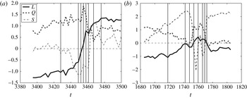
The evolution of the amplitudes in figure 14(a) allows us to provide a more accurate description of the standard reversal mechanism. We checked that the features reported below were characteristic of all reversals of this type. At the beginning of the reversal, the two-roll mode
 $S$
is very small and its amplitude is negative, but it crosses zero (figure 12
a) and starts to increase significantly (figure 12
b), while mode
 $L$
starts to decrease. As the mode
 $L$
reaches zero (figure 12
c), the quadrupolar mode
 $Q$
becomes dominant (figure 12
d), then decreases (figure 12
e). The double-roll, symmetry-breaking mode
 $S$
reaches a plateau (figure 12
b–f) then experiences a strong sign switch, while the quadrupolar mode becomes less intense and reaches a minimum value (figure 12
g). Note that while
 $L$
has changed sign, the sign of
 $Q$
remains constant, so that the corner rolls move to the opposite diagonal of the square cell. The amplitude of the mode
 $S$
then tends to decrease, while the modes
 $L$
and
 $Q$
settle towards their equilibrium values (figure 12
g).

In a similar fashion, figure 14(b) provides a compact description of the flow dynamics during the cessation. At the beginning of the sequence, the flow is dominated by the single roll mode
 $L$
(figure 13
a). The collapse of the single roll mode
 $L$
occurs as the amplitude of the mode
 $S$
increases significantly. Modes
 $L$
and
 $Q$
then collapse (figure 13
b,c), while mode
 $S$
increases significantly. Mode
 $Q$
then increases, while mode
 $L$
and mode
 $S$
cross the zero axis almost simultaneously (figure 13
d). During the second part of the sequence (figure 13
d–h), the double roll mode changes orientation frequently, which corresponds to a sign switch in mode
 $S$
. We note that the horizontal two-roll flow is correctly recovered (figure 13
a,d,g,h), but the reconstruction fails when the main axis of the rolls rotates and becomes vertical. This is consistent with the fact that vertical two-roll modes (mode 5 in the velocity-based and mixed decomposition, mode 7 in the temperature-based decomposition) are excluded from the truncation. At the end of the sequence, the double-roll mode dominates the flow, while the large-scale circulation and quadrupolar mode are still weak (figure 13
g,h).
To sum up, both reversals and cessations involve a collapse of the
 $L$
mode associated with an increase in the
 $S$
mode. The distinction we make between these two types of events is based only on the length of this phase and it is therefore unlikely that they correspond to distinct physical mechanisms. We now determine whether the dynamics described above can be captured with a low-dimensional model.
4. Model derivation
4.1. Mode interaction
We now examine whether the dynamics of the flow can be reproduced with a low-dimensional model derived from POD, as has been done for several types of turbulent flows Aubry et al. (Reference Aubry, Holmes, Lumley and Stone1988), Sirovich & Park (Reference Sirovich and Park1990) and Bailon-Cuba et al. (Reference Bailon-Cuba, Emran and Schumacher2010). The coefficients of the model are typically computed from Galerkin projection of the equations of motion onto the basis of eigenfunctions. A closure hypothesis is then used to represent the effect of the unaccounted scales on the ones included in the truncation. In all that follows we will use the mixed formulation, i.e. will use a single coefficient to describe the behaviour of both velocity and temperature modes. The similarities noted in figure 11 provide some justification for doing this. We therefore write
 $$\begin{eqnarray}\left[\begin{array}{@{}c@{}}\boldsymbol{u}\\ {\it\theta}\end{array}\right]=\mathop{\sum }_{n=1}^{N}a^{n}\left[\begin{array}{@{}c@{}}\underline{{\it\phi}}_{\boldsymbol{u}}\\ {\it\phi}_{{\it\theta}}\end{array}\right]\!.\end{eqnarray}$$
The decomposition is injected into the equations of motion (2.5) and these equations are then projected onto the set of eigenfunctions
 $\underline{{\it\phi}}^{n}$
(details can be found in Holmes et al. (Reference Holmes, Lumley and Berkooz1996) or Podvin & Sergent (Reference Podvin and Sergent2012)). This leads to a model of the following form:
 $$\begin{eqnarray}{\dot{a}}^{n}=L_{mn}a^{m}+Q_{mpn}a^{m}a^{p}+T_{n},\end{eqnarray}$$
where we have the following.
-
(i) We use
$L_{mn}=L_{mn}^{d}+L_{mn}^{b}$
to represent the combined effect of dissipation
$L_{mn}^{d}$
and buoyancy
$L_{mn}^{b}$
. We have (4.3)where
$$\begin{eqnarray}L_{mn}^{d}=\frac{1}{\mathit{Ra}^{1/2}}\int (\mathit{Pr}\boldsymbol{{\rm\nabla}}\underline{{\it\phi}}_{\boldsymbol{u}}^{n}:(\boldsymbol{{\rm\nabla}}\underline{{\it\phi}}_{\boldsymbol{u}}^{m})^{\text{T}}+\boldsymbol{{\rm\nabla}}{\it\phi}_{{\it\theta}}^{n}\boldsymbol{\cdot }\boldsymbol{{\rm\nabla}}{\it\phi}_{{\it\theta}}^{m})\,\text{d}\underline{x}\end{eqnarray}$$
$T$
represents the transposition operator, and (4.4)
$$\begin{eqnarray}L_{mn}^{b}=\int ({\it\phi}_{{\it\theta}}^{n}{\it\phi}_{w}^{m})\,\text{d}\underline{x}.\end{eqnarray}$$
-
(ii) The quadratic terms
$Q_{mpn}$
(which cannot be confused with the quadrupolar mode
$Q$
) are defined as (4.5)They correspond to the transport of the Reynolds stress as well as that of the convective heat flux. Only the contribution from the resolved modes is included directly in the model.
$$\begin{eqnarray}Q_{mpn}=\int [(\underline{{\it\phi}}_{\boldsymbol{u}}^{m}\boldsymbol{\cdot }\boldsymbol{{\rm\nabla}}\underline{{\it\phi}}_{\boldsymbol{u}}^{p}+\underline{{\it\phi}}_{\boldsymbol{u}}^{p}\boldsymbol{\cdot }\boldsymbol{{\rm\nabla}}{\it\phi}_{\boldsymbol{u}}^{m})\boldsymbol{\cdot }\underline{{\it\phi}}_{\boldsymbol{u}}^{n}+(\underline{{\it\phi}}_{\boldsymbol{u}}^{m}\boldsymbol{\cdot }\boldsymbol{{\rm\nabla}}\underline{{\it\phi}}_{{\it\theta}}^{p}+\underline{{\it\phi}}_{\boldsymbol{u}}^{p}\boldsymbol{\cdot }\boldsymbol{{\rm\nabla}}{\it\phi}_{{\it\theta}}^{m}){\it\phi}_{{\it\theta}}^{n}]\,\text{d}\underline{x}.\end{eqnarray}$$
-
(iii) Here
$T_{n}$
represents the contribution of the unresolved modes to the evolution of the modes included in the truncation. Different types of closures can be used. The classical approach pioneered by Aubry et al. (Reference Aubry, Holmes, Lumley and Stone1988) in the case of a turbulent channel flow consists in using a simple dissipative model based on a Smagorinsky-like hypothesis. It has been widely applied (see Podvin & Le Quéré (Reference Podvin and Le Quéré2001) and Bailon-Cuba et al. (Reference Bailon-Cuba, Emran and Schumacher2010)) and results in additional linear terms. We note that an alternative to a stabilizing eddy viscosity has been recently proposed by Balajewicz, Dowell & Noack (Reference Balajewicz, Dowell and Noack2013) and relies on the addition of a constraint on the resolved turbulent kinetic energy in the optimization process. However, it seems to have been applied to 2D flows so far.The unresolved modes take energy away from the resolved modes, and the rate at which they extract this energy should increase with the amplitude of the resolved modes. In the absence of convection, the turbulent eddy viscosity is typically assumed to be proportional to the local strain rate
$s_{ij}$
(4.6)This approximation is consistent with the recent findings of with a recent paper by Osth et al. (Reference Osth, Noack, Krajnoci, Borée and Barros2014) which makes the case for a nonlinear subscale representation in low-dimensional models. They show that model robustness is achieved for representations of the type
$$\begin{eqnarray}{\it\nu}_{T}\sim C|s_{ij}s_{ij}|^{1/2}.\end{eqnarray}$$
(4.7)where
$$\begin{eqnarray}{\it\nu}_{T}\sim C^{\prime }|k_{{<}}|^{1/2},\end{eqnarray}$$
$k_{{<}}$
represents the energy of the resolved modes
$a^{n}$
.
In the case of natural convection, a simple gradient diffusion hypothesis for the turbulent heat fluxes is generally not acceptable (Choi & Kim Reference Choi and Kim2012). A better mode for the turbulent heat fluxes is given by Ince & Launder (Reference Ince and Launder1989):
(4.8)where
$$\begin{eqnarray}\langle {\it\theta}u_{i}\rangle =-C_{{\it\theta}}\frac{k}{{\it\epsilon}}\langle u_{i}u_{k}\rangle \frac{\partial \langle {\it\theta}\rangle }{\partial x_{k}}\end{eqnarray}$$
$k$
is the turbulent kinetic energy and
${\it\epsilon}$
is the dissipation. This means that as a first approximation, it is possible to relate the evolution of the unresolved turbulent heat fluxes to that of the unresolved turbulent stresses.
We therefore choose to generalize Osth et al.’s approach to thermal convection flows, i.e. to use (4.7). One further simplification was made as we observed that the temporal variations of the energy of the first POD modes were typically small compared to its mean value: the normalized standard deviation was less than 0.25. One can then write
(4.9)with
$$\begin{eqnarray}k(t)=\langle k\rangle +\tilde{k}(t)\end{eqnarray}$$
$|\tilde{k}(t)|\ll \langle k\rangle$
. In this case, we can make the approximation (4.10)
$$\begin{eqnarray}\sqrt{k(t)}=\sqrt{\langle k\rangle }(1+\tilde{k}(t)/\langle k\rangle )^{1/2}\sim \sqrt{\langle k\rangle }\left(1+\frac{1}{2}\frac{\tilde{k}(t)}{\langle k\rangle }\right)=\frac{\sqrt{\langle k\rangle }}{2}\left(1+\frac{k(t)}{\langle k\rangle }\right).\end{eqnarray}$$
The eddy viscosity therefore contains a constant and a quadratic part, which yields linear terms and cubic terms in the equations. If all cubic terms are negative, this ensures global stability of the model. We note that cubic terms also appeared in the low-dimensional model of turbulent channel flow Aubry et al. (Reference Aubry, Holmes, Lumley and Stone1988) with a different derivation, which was a feedback term in the expression of the mean velocity profile.


The final form of the model is, therefore,
 $$\begin{eqnarray}{\dot{a}}^{n}=({\it\lambda}_{mn}-{\it\alpha}_{mnp}{\it\delta}_{mn}|a^{p}|^{2})a^{m}+Q_{mpn}a^{m}a^{p}.\end{eqnarray}$$
We emphasize that the values of the coefficients are determined by the shape and magnitude of the POD eigenfunctions and therefore contain implicit information about the specific physics of the flow. The coefficients
 $Q_{mnp}$
, which characterize how the different eigenfunctions interact with each other, can be evaluated directly from computation of the resolved POD modes. The linear term
 ${\it\lambda}_{mn}$
contains a contribution from the resolved and unresolved modes, while the cubic term
 ${\it\alpha}_{mnp}$
contains exclusively contributions from the unresolved POD modes. Both kinds of terms are not known a priori. We now consider lowest-order truncations of (4.11).
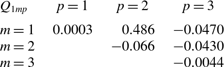
Quadratic coefficients
 $Q_{1mp}$
(only the upper part of the symmetric matrix is represented).

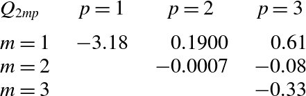
Quadratic coefficients
 $Q_{2mp}$
(only the upper part of the symmetric matrix is represented).

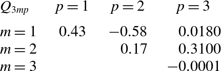
Quadratic coefficients
 $Q_{3mp}$
(only the upper part of the symmetric matrix is represented).

4.2. Minimal truncations
4.2.1. Model coefficients
Tables 2–4 contain the interaction coefficients
 $Q_{mnp}$
for the first three modes. The dominant terms for each mode are given in bold. They correspond to those we will choose to retain in the model. We checked that the modes selected for nonlinear interaction did not depend on the POD formulation by computing the interactions for velocity-based modes, as well as temperature modes.
The quadratic interactions are entirely determined from the POD modes, which makes our approach different from the symmetry-based derivation of Gissinger, Dormy & Fauve (Reference Gissinger, Dormy and Fauve2010) and Gallet et al. (Reference Gallet, Hérault, Laroche, Pétrélis and Fauve2012). In these models, the evolution of each mode is governed by the quadratic interaction between the other two modes. In our model, the quadratic interaction governing the evolution of the large-scale circulation involves the large-scale circulation and the quadrupolar mode, while the dominant term in the evolution of the second mode (the quadrupolar flow) is the interaction of the first mode with itself.
Table 5 contains the resolved parts
 $L_{mn}^{d},L_{mn}^{b}$
and their sum
 $L_{mn}$
for the first three modes. We note that the diagonal term
 $L_{nn}$
is dominant for the first two modes. However, for the third mode
 $S$
, a contribution from the first mode
 $L$
is significant. We checked that the buoyancy matrix
 $L_{mn}^{b}$
only had positive eigenvalues, which is consistent with the fact that buoyancy is a source term for the dynamics. The eigenvector associated with the largest buoyancy eigenvalue has a dominant component in the quadrupolar mode, but has also significant components in the first and third mode.
We now consider truncations of the model. The amplitudes
 $a^{n}$
will now be considered in non-normalized form, since the expression
 $k_{{<}}$
used to represent the effect for the unresolved scales is based on the non-normalized coefficients (but they will be normalized again for comparison with the amplitudes from the DNS).
4.2.2. Two-mode model
As a first step, we first consider a system limited to the first two modes, i.e. the large-scale circulation and the quadrupolar flow. This model is formally reminiscent of the classic two-mode interaction (see below) found in a variety of problems such as the turbulent boundary layer of a channel (Aubry et al.
Reference Aubry, Holmes, Lumley and Stone1988; Podvin & Lumley Reference Podvin and Lumley1998) or Couette flow (Smith, Moehlis & Holmes Reference Smith, Moehlis and Holmes2005). These flows are characterized by the presence of
 $O(2)$
symmetry, and it has been shown that it is sufficient to consider the evolution of these modes (Armbruster, Guckenheimer & Holmes Reference Armbruster, Guckenheimer and Holmes1988) to obtain reversals, which appear as heteroclinic cycles. However, in our case there is no
 $O(2)$
symmetry, only a reflection symmetry is present. Moreover, in the previous situations, the mode with the smaller wavelength changes sign during a sharp increase of the energy in the larger ones, which is a very different situation from that observed here. Here the ‘flipping’ mode has the larger wavelength, while the quadrupolar mode does not change sign.
If we consider (4.11) and retain only the first two modes (
 $L$
and
 $Q$
), we then obtain the following model:
 $$\begin{eqnarray}\displaystyle & \dot{L}=({\it\chi}-{\it\alpha}r^{2})L-c_{1}LQ & \displaystyle\end{eqnarray}$$
 $$\begin{eqnarray}\displaystyle & \dot{Q}=({\it\mu}-{\it\beta}r^{2})Q+c_{2}L^{2} & \displaystyle\end{eqnarray}$$
 $r^{2}=L^{2}+Q^{2}$
. The coefficients
 $c_{1}$
and
 $c_{2}$
are evaluated from computation of the quadratic coefficients since
 $c_{1}=-Q_{121}/\sqrt{{\it\lambda}_{2}}$
and
 $c_{2}=Q_{112}\sqrt{{\it\lambda}_{2}}/{\it\lambda}_{1}$
. Here
 ${\it\chi},{\it\mu},{\it\alpha},{\it\beta}$
have to be determined. We assume that
 ${\it\alpha}$
and
 ${\it\beta}$
are positive to ensure the global stability of the system.
Linear coefficients
 $L_{nm}^{b}$
,
 $L_{nm}^{d}$
and
 $L_{nm}^{b}+L_{nm}^{d}$
.

Between reversals the
 $L$
and the
 $Q$
modes are nearly constant and non-zero, which leads us to look for equilibria such that
 $(L_{0}\neq 0,Q_{0}\neq 0)$
, which we will call
 $LQ$
-equilibria.
The
 $LQ$
-equilibria satisfy
 $$\begin{eqnarray}{\it\chi}-{\it\alpha}r_{0}^{2}=c_{1}Q_{0}\end{eqnarray}$$
and
 $$\begin{eqnarray}{\it\mu}-{\it\beta}r_{0}^{2}=-c_{2}L_{0}^{2}/Q_{0}\end{eqnarray}$$
where
 $r_{0}^{2}=L_{0}^{2}+Q_{0}^{2}$
. The stability of these fixed points can be determined from their Jacobian
 $$\begin{eqnarray}\left[\begin{array}{@{}cc@{}}-2{\it\alpha}L_{0}^{2} & -2{\it\alpha}L_{0}Q_{0}-c_{1}L_{0}\\ -2{\it\beta}L_{0}Q_{0}+2c_{2}L_{0} & -2{\it\beta}Q_{0}^{2}-c_{2}L_{0}^{2}/Q_{0}\end{array}\right]\!.\end{eqnarray}$$
We note that the eigenvalues of the Jacobian are the same when
 $L_{0}\rightarrow -L_{0}$
. If
 $T$
is the trace and
 $D$
is the determinant of the matrix, the eigenvalues of the matrix are
 $T/2\pm ((T^{2}/4)-D)^{1/2}$
. For a reversal to occur, we need the fixed point to be a saddle point, which implies that the determinant is negative, since the trace is already negative. After some computation, this gives us the condition on
 ${\it\beta}>c_{2}/Q_{0}(c_{1}+2{\it\alpha}Q_{0}+{\it\alpha}L_{0}^{2}/Q_{0}/({\it\alpha}Q_{0}+c_{1}))$
.
We picked an arbitrary value of
 ${\it\alpha}=1$
, and chose
 ${\it\beta}$
so that the condition was verified.
In all the tests we ran, the system was attracted to pure
 $Q$
modes of the form
 $(L,Q)=(0,({\it\mu}/{\it\beta})^{1/2})$
. Combining (4.15) and (4.14) yields
 $$\begin{eqnarray}r_{0}^{2}=\frac{{\it\chi}}{{\it\alpha}}-\frac{c_{1}Q_{0}}{{\it\alpha}}=\frac{{\it\mu}}{{\it\beta}}+c_{2}\frac{L_{0}^{2}}{Q_{0}{\it\beta}}.\end{eqnarray}$$
Since
 $Q_{0}>0$
this means that
 ${\it\chi}/{\it\alpha}<{\it\mu}/{\it\beta}$
, i.e. that all pure
 $Q$
equilibria are nodes. This negates the possibility of a flipping mechanism for mode
 $a^{1}$
.
4.2.3. Three-mode model
We now add the extra mode
 $S$
(
 $a^{3}$
in the mixed formulation), which represents the double-roll mode. As seen earlier, this mode breaks the flow
 $S_{x}$
-symmetry, unlike the first two modes.
Keeping only the first three modes in the truncation, equation (4.11) then reads
 $$\begin{eqnarray}\displaystyle & \dot{L}=({\it\chi}-{\it\alpha}r^{2})L-c_{1}LQ & \displaystyle\end{eqnarray}$$
 $$\begin{eqnarray}\displaystyle & \dot{Q}=({\it\mu}-{\it\beta}r^{2})Q+c_{2}L^{2}+c_{3}LS & \displaystyle\end{eqnarray}$$
 $$\begin{eqnarray}\displaystyle & {\dot{S}}=({\it\nu}-{\it\gamma}r^{2})S+({\it\nu}^{\prime }-{\it\gamma}^{\prime }r^{2})L-c_{4}LQ & \displaystyle\end{eqnarray}$$
 $r^{2}=L^{2}+Q^{2}+S^{2}$
,
 $c_{3}=Q_{132}({\it\lambda}_{1}{\it\lambda}_{3}/{\it\lambda}_{2})^{1/2}$
and
 $c_{4}=-Q_{123}({\it\lambda}_{1}{\it\lambda}_{2}/{\it\lambda}_{3})^{1/2}$
. We can see that the signs of the quadratic terms ensure that the energy is redistributed among the modes. If the linear and cubic terms are set to zero, one has
 $$\begin{eqnarray}\frac{\text{d}}{\text{d}t}(Q^{2}+c_{2}/c_{1}L^{2}+c_{4}/c_{3}S^{2})=0.\end{eqnarray}$$
Again, we assume
 ${\it\alpha},{\it\beta},{\it\gamma},{\it\gamma}^{\prime }$
to be positive to ensure the global stability of the system. Between reversals, the dominant modes are the quadrupolar flow
 $Q$
and the large-scale circulation
 $L$
, which are nearly constant as a first approximation. This suggests that we look for fixed points of the form
 $(L_{0},Q_{0},0)$
, which we will also denote
 $LQ$
-equilibria. We will denote
 $LQ_{+}$
(respectively
 $LQ_{-}$
) the equilibrium such that
 $L_{0}>0$
(respectively
 $L_{0}<0$
). These fixed points satisfy (4.14) and (4.15). The stability of these points is given by the eigenvalues of the Jacobian:
 $$\begin{eqnarray}M_{LQ}=\left[\begin{array}{@{}ccc@{}}-2{\it\alpha}L_{0}^{2} & -2{\it\alpha}Q_{0}L_{0}-c_{1}L_{0} & 0\\ 2c_{2}L_{0}-2{\it\beta}Q_{0}L_{0} & -2{\it\beta}Q_{0}^{2}-c_{2}L_{0}^{2}/Q & +c_{3}L_{0}\\ -c_{4}Q_{0}+{\it\nu}^{\prime }-{\it\gamma}^{\prime }(Q_{0}^{2}+3L_{0}^{2}) & -c_{4}L_{0}-2{\it\gamma}^{\prime }Q_{0}L_{0} & {\it\nu}-{\it\gamma}(L_{0}^{2}+Q_{0}^{2})\end{array}\right]\!.\end{eqnarray}$$
We can check that the eigenvalues of
 $M_{LQ}$
are independent of the sign of
 $L_{0}$
. Let
 ${\it\sigma}_{MLQ}$
be the eigenvalue of
 $M_{LQ}$
with largest real part. Heteroclinic excursions can occur if
 ${\it\sigma}_{MLQ}$
has a positive real part.
Similarly, during standard reversals, the symmetry-breaking mode
 $S$
becomes important, while the large-scale circulation
 $L$
collapses and the quadrupolar vortex flow
 $Q$
sharply decreases after a short increase, as was seen in figure 14. This suggests that we look for another type of fixed point of the form
 $(0,0,S_{0})$
, which we will call a
 $S$
-equilibrium and will denote
 $S_{+}$
or
 $S_{-}$
depending on the sign of
 $S_{0}$
. We note that the existence of a fixed point in this subspace would be consistent with the occurrence of the cessation events dominated by the symmetry breaking mode observed in figure 4. In our model, a stationary pure symmetry-breaking mode satisfies
 $S_{0}=\pm ({\it\nu}/{\it\gamma})^{1/2}$
and its stability is determined by
 $$\begin{eqnarray}M_{S}=\left[\begin{array}{@{}ccc@{}}{\it\chi}-{\it\alpha}S_{0}^{2} & 0 & 0\\ 0 & {\it\mu}-{\it\beta}S_{0}^{2} & 0\\ {\it\nu}^{\prime }-{\it\gamma}^{\prime }S_{0}^{2} & 0 & -2{\it\gamma}S_{0}^{2}\end{array}\right]\!.\end{eqnarray}$$
We denote by
 ${\it\sigma}_{MS}$
the eigenvalue of
 $M_{S}$
with largest real part. For
 ${\it\sigma}_{MS}$
to have a positive real part, we need
 ${\it\chi}-{\it\alpha}({\it\nu}/{\it\gamma})>0$
or
 ${\it\mu}-{\it\beta}({\it\nu}/{\it\gamma})>0$
.
The eigenvalues of
 $M_{LQ}$
and
 $M_{S}$
only depend on the values of
 $({\it\alpha},{\it\beta},{\it\gamma},{\it\gamma}^{\prime })$
, which are not known a priori. The parameters
 $({\it\chi},{\it\mu},{\it\nu}^{\prime })$
can then be evaluated using approximated values of the
 $LQ$
equilibrium in the DNS. We did not use the DNS value of the
 $S$
equilibrium to adjust the coefficients in the model, as neglected higher-order modes become important during reversals, so that the value of
 $S$
predicted by the model is likely to be different from the simulation (an overestimation is expected). The parameter
 ${\it\nu}$
was simply chosen large enough so that
 $M_{S}$
could have one positive eigenvalue, which meant that either
 ${\it\nu}<{\it\chi}{\it\gamma}/{\it\alpha}$
or
 ${\it\nu}<{\it\mu}{\it\gamma}/{\it\beta}$
. In practice, we chose a value for
 ${\it\nu}$
slightly smaller than
 ${\it\chi}{\it\gamma}/{\it\alpha}$
.
A parametric study in the (
 ${\it\alpha},{\it\beta},{\it\gamma},{\it\gamma}^{\prime }$
) domain was therefore carried out to determine the conditions of existence of saddle equilibria, and to establish whether the dynamics displayed by the model held over a wide range of parameters. The variations of
 ${\it\sigma}_{MLQ}$
and
 ${\it\sigma}_{MS}$
were computed for
 ${\it\alpha}$
,
 ${\it\beta}$
and
 ${\it\gamma}$
in the range
 $[0.05,0.25]$
. In that domain we found (not shown) that both
 $LQ$
- and
 $S$
-equilibria were unstable. The most unstable eigenvector of
 $M_{LQ}$
has a dominant component along the
 $S$
axis, while the most unstable eigenvector of
 $M_{S}$
is in the
 $Q=0$
plane and is of the form
 $(l\neq 0,0,s\neq 0)$
.
We note that the existence of saddle equilibria is not a sufficient condition for the existence of heteroclinic connections. Moreover, such connections are typically not robust in the presence of small perturbations. However. in our case, we found structurally stable near-heteroclinic connections, which we will now describe. When the model admitted ‘pure’
 $LQ$
- and
 $S$
-equilibria as saddle points, we found close to each equilibrium a ‘mixed’ stable equilibrium respectively of the form
 $(L,Q,{\it\epsilon}_{S})$
and
 $({\it\epsilon}_{L},{\it\epsilon}_{Q},S)$
where
 ${\it\epsilon}_{L},{\it\epsilon}_{Q},{\it\epsilon}_{S}$
were non-zero but relatively small. We will respectively denote these equilibria
 $LQ_{\pm }^{{\it\epsilon}}$
and
 $S_{\pm }^{{\it\epsilon}}$
. These stable equilibria could either be nodes or sinks. The distance between the ‘pure’ and the ‘mixed’ equilibria depended on the model parameters, and was found to decrease as
 ${\it\gamma}^{\prime }$
increased (hence, the relatively high value of
 ${\it\gamma}^{\prime }$
considered below). The key element, which was found to hold for the range of parameters considered, was that each pure saddle point was connected to one mixed stable equilibrium of each type. To be specific,
 $LQ_{+}$
was connected to
 $LQ_{+}^{{\it\epsilon}}$
for perturbations with a positive component along the
 $S$
axis and to
 $S_{-}^{{\it\epsilon}}$
for perturbations with a negative component. In the same fashion.
 $S_{-}$
was connected to
 $LQ_{-}^{{\it\epsilon}}$
for perturbations with a negative
 $L$
component and to
 $S_{+}^{{\it\epsilon}}$
for perturbations with a positive component. The dependence of the connections on the relative signs of
 $S$
and
 $L$
reflects the importance of the relative orientation of the double-roll with respect to the single large-scale circulation. Analogous relationships can be obtained for
 $LQ_{-}$
and
 $S_{+}$
by reversing all signs.
We thus propose the following scenario for the reversals: the system starting near the
 $LQ_{+}$
equilibrium is attracted to the
 $S_{-}^{{\it\epsilon}}$
equilibrium, then kicked away from it through the action of noise towards the nearby saddle point
 $S_{-}$
on the
 $S$
axis, from which it will be sent back near the
 $S=0$
plane towards the
 $LQ_{-}^{{\it\epsilon}}$
equilibrium. The presence of noise will then kick it out towards the
 $LQ_{-}$
saddle point, from where it travels away towards the equilibrium
 $S_{+}^{{\it\epsilon}}$
, when it can be kicked out again by noise towards
 $S_{+}$
, which will send it away towards
 $LQ_{+}^{{\it\epsilon}}$
, i.e. in the neighbourhood of our original starting point. The part of the cycle between
 $LQ_{+}$
and
 $LQ_{-}$
, with a relatively short stay near the
 $S_{\pm }$
equilibrium corresponds to a standard reversal. A cessation corresponds to the system hovering near one of the
 $S_{\pm }$
equilibria. This dynamical picture supports that the idea that the same physical mechanism is involved in reversals and cessations.
In the remainder of the paper, we adopt fixed values for
 $({\it\alpha},{\it\beta},{\it\gamma},{\it\gamma}^{\prime })$
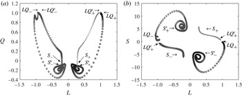
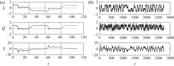
, which are indicated in table 6. Figure 15 presents an illustration of the near-heteroclinic cycle described above. The cycle was obtained by integrating the model from an initial condition close to the saddle equilibrium
 $LQ_{+}$
and then perturbing the system by using
 $L\rightarrow -L$
and
 $S\rightarrow -S$
as the system respectively approached the
 $S_{{\it\epsilon}}$
and
 $LQ_{{\it\epsilon}}$
stable equilibria. The time histories corresponding to the phase portraits are given in figure 16(a). The deterministic, temporally isolated perturbations corresponding to the straight lines in figure 16(a) mimic the effect of noise.
Illustration of the near-heteroclinic cycle (see the text): (a)
 $(L,Q)$
plane; (b)
 $(L,S)$
plane.


(a) Histories of the POD amplitudes integrated from the model without noise and represented in figure 15. Each vertical line corresponds to the start of a new integration. (b) Histories of the POD amplitudes integrated from the model with a noise perturbation level of 0.16 for each component.

Figure 16(b) shows mode amplitude histories when random perturbations are added to the model. The initial condition was taken from the DNS, and a random Gaussian perturbation with an arbitrary amplitude of 0.16 was added to each component. Both standard reversals and cessations are observed in the time evolution of the amplitudes (note, for instance, the cessation reversal at
 $t\sim 1400$
). For reversal cases, we were able to predict the reversal of the large-scale circulation, associated with an excursion of the quadrupolar mode and of the symmetry-breaking mode. We note that the low-dimensional model predicts a collapse of the quadupolar mode, which is briefly observed in the DNS. However, we do not predict the increase in the
 $Q$
mode after the reversal. In the cessation case, we reproduced the excursion of the double-roll mode and the collapse of the large-scale circulation. However, the model is unable to capture the rotation of the two rolls, due to our limited truncation. For both reversals, the excursions and equilibrium values of the symmetry-breaking mode are much higher than those observed in the DNS. As noted earlier, this effect is consistent with the absence of higher-order modes.
Figure 16(a) indicates that the travel time from the neighbourhood of
 $L_{+}$
to that of
 $S_{-}^{{\it\epsilon}}$
(and equivalently from
 $L_{-}$
to
 $S_{+}^{{\it\epsilon}}$
) is approximately 2–3 convective units, while that from the
 $S_{-}$
to the
 $L_{+}^{{\it\epsilon}}$
equilibrium (and from
 $S_{+}$
to
 $L_{-}$
) is approximately 6 convective units. The duration of the standard reversal in the model is therefore approximately 8–9 convective units or about
 ${\it\tau}_{E}$
, which is in good agreement with the mean time of 11 units reported for the simulation in § 2.3.
A related viewpoint is given by the distribution of the residence times spent by the system away from the
 $L$
equilibria. During these times we have
 $|L|\leqslant L_{m}$
where
 $L_{m}$
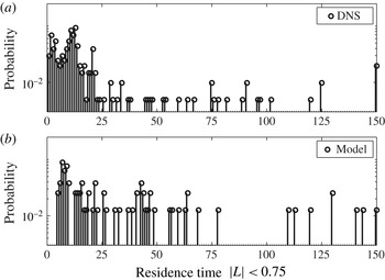
is some threshold. This corresponds to either standard reversals or cessations. The distribution (with a bin width of 1 time unit) is shown in figure 17 with
 $L_{m}=0.75$
for both the DNS (a) and the model (b). In the DNS it is characterized by a dense cluster of low values in the range
 $[0,20]$
time units while higher, less frequent values are observed above 25 time units. By definition the first region is associated with standard reversals, while cessations are associated with the second region. The absence of a clear boundary suggests that standard reversals and cessations respectively represent the ‘head’ and the tail of the distribution of a single phenomenon.
Distribution of the time spent by the system near the
 $L=0$
plane
 $|L|<0.75$
: (a) DNS; (b) model.

In the model and the simulation the distributions reach their absolute maximum at 8.5 and 11.5 convective units, respectively. Maxima around 10 convective units were also identified for thresholds
 $L_{m}$
in the range
 $[0.6,0.9]$
, which shows some robustness for the criterion (as can be expected, the location of the maximum tends to decrease slightly as the threshold decreases). A first relative maximum in the distribution of the DNS can be noticed at approximately 2 time units. It represents variations of the
 $L$
mode which typically follow a reversal (as the newly formed large-scale circulation rearranges itself). The model is not able to reproduce these details of the reversal, which involves higher-order modes, hence the absence of this lower peak. Moreover, the interface between the two flow mode transitions is even more blurred in the model, which tends to overpredict the occurrence of cessations.
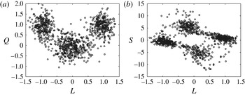
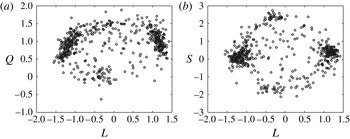
The flow mode transitions are also present in the phase portraits of the noisy integration, which are shown in figure 18 and can be compared to the corresponding phase portraits of the simulation in figure 19. Cessations and standard reversals are associated with the region of space close to the
 $L=0$
axis. Some agreement can be noted both in the
 $(L,Q)$
space and in the
 $(L,S)$
space, where clusters of points corresponding to
 $LQ$
- and
 $S$
-equilibria can be identified. However, the magnitude of the
 $S$
mode tends to be larger in the model than in the simulation. Again, this is likely to be due to the absence of small scales in the model.
Heteroclinic cycle corresponding to the time histories in figure 16: (a)
 $(L,Q)$
plane; (b)
 $(L,S)$
plane.

Phase portrait in the DNS: (a)
 $(L,Q)$
plane; (b)
 $(L,S)$
plane.

As was done in § 2.3 with the angular momentum
 $L_{2D}$
, the average time between standard reversals can be estimated from the number of zero crossings of the POD mode
 $L$
. Figure 20 shows the distribution of the time intervals between zeros of
 $L$
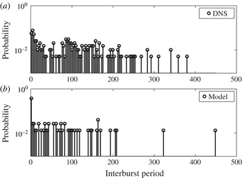
in both the simulation and the model with a noise level of 0.12. Bins of three convective time units are used. We observe a maximum in the distribution near the origin for the DNS which corresponds to a single peak value for the model. As stated earlier, these short intervals correspond to crossings of the zero axis which occur on a faster time scale than the duration of a standard reversal. This means that these zeros are associated with cessations (several crossings may occur during a typical cessation).
Distribution of the time interval between zeros of
 $L$
: (a) DNS; (b) model.

A second dense cluster of time scales can be observed in the DNS with a maximum at approximately 90 time units. The cut-off between the two regions, which can be identified by a relative decrease in the probability density, seems to be approximately 50 time units: there is no sharp boundary. The separation between the two regions is even more difficult to identify in the model, where a relatively uniform distribution is observed up to approximately 200 time units. The average time between reversals in the model was computed by excluding intervals lower than the duration of the reversal (taken to be 10 units). It was found to be approximately 80 time units, for a noise level of 0.16, which is approximately a factor of 1.6 smaller than the value of 120 observed in the simulation. This discrepancy fell to 1.2 for a lower noise level of 0.12.
Stone & Holmes (Reference Stone and Holmes1989) have shown that the time
 ${\it\tau}$
spent by the system near an equilibrium in a region of size
 ${\it\epsilon}$
should scale on average as
 $$\begin{eqnarray}{\it\tau}\sim \frac{1}{{\it\sigma}^{u}}\log ({\it\epsilon}/{\it\delta})+O(1),\end{eqnarray}$$
where
 ${\it\sigma}^{u}$
is the magnitude of the unstable eigenvalue and
 ${\it\delta}$
is the noise level in the system. It might therefore be possible to adjust both the coefficients of the model and the noise level so that the time spent by the system near an equilibrium matches the inter-reversal time observed in the simulation. However, this was not attempted. We only checked that lower noise amplitudes resulted in a longer time interval between reversals.
5. Conclusion
POD was applied to the numerical simulation of Rayleigh–Bénard convection in a square cell at a Rayleigh number of
 $\mathit{Ra}=5\times 10^{7}$
, for which reversals of the large-scale circulation were observed. Two types of stable flow patterns, a single roll with two small rolls in the opposite corners and two horizontally stacked vortices, were identified in the simulation. During reversals, they were respectively associated to transient features such as a quadrupolar flow and two vertical rolls. Two different kinds of mechanisms, corresponding to the growth of a corner flow and rotation effects, appeared to be involved in the transition process.
Three main modes were identified in the POD decomposition of the velocity as well as that of the temperature. The most energetic mode in the velocity-based decomposition was the antisymmetric large-scale circulation
 $L$
, the sign of which switches intermittently. The most energetic mode in the temperature-based decomposition was a symmetric quadrupolar velocity field
 $Q$
associated with the mean temperature. The third most important mode was a symmetry-breaking, double-roll mode
 $S$
. Most of the heat flux was concentrated along the vertical walls and was dominated by the contributions of the first two modes: the large-scale circulation was associated with a heat flux in the center section of the vertical boundary layers, while the flux corresponding to the quadrupolar flow was maximal near the horizontal walls.
Changes in the large-scale organization of the flow were described in terms of the amplitudes of the POD modes. During such changes, all structures experienced violent excursions in both directions and the flow symmetry was broken. Two types of events, standard reversals and cessations, appear to be taking place: in standard reversals, which were most commonly observed, the large-scale circulation switched rapidly between two near-stationary, opposite states, and the double-roll mode went through a considerable excursion which lasted approximately 10 convective units. During less-frequent cessations occurring on a longer time scale, the large-scale circulation collapsed and the double-roll mode became dominant. The only distinction we can make between the two types of events is based on the duration of the excursions. The dynamics of the POD modes in both processes is similar, and it is likely that they correspond to a single physical mechanism.
We attempted to capture these mechanisms with a reduced-order dynamical system to which noise is added. The quadratic interaction terms were determined directly from Galerkin projection of the equations onto the POD modes. The model involves the large-scale circulation
 $L$
, the quadrupolar flow
 $Q$
and the symmetry-breaking, double-roll mode
 $S$
. The skeleton of the dynamics is a noisy near-heteroclinic cycle linking ‘pure’, saddle equilibria of
 $LQ$
- and
 $S$
-type to mixed-mode, stable equilibria respectively close to the
 $S$
- and
 $LQ$
-pure saddle points. The connection from a stable equilibrium to a nearby saddle point occurs through noise, which models the action of higher-order modes.
Despite the limitations of our model, which include the severity of the truncation and the crudeness of the closure model, we were able to reproduce key features of the large-scale evolution of the flow associated with standard reversals and cessations. The model captures the collapse of the large-scale circulation, the decrease of the quadrupolar flow and the growth of the symmetry-breaking mode common to these events.
Under the action of noise, the system can transit rapidly through one
 $S$
-type equilibrium between two
 $L$
-type equilibria, reproducing a standard reversal. The time scale of the reversal in the model matches that of the simulation. The interval between reversals can be adjusted in the model to match that of the simulation by adding an appropriate level of noise. When the system remains trapped near one of the
 $S$
-equilibria, a cessation occurs. The duration of the cessations also depends on the amount of noise present in the system. Over a range of noise levels (0.1–0.16) we found that the model was able to capture relatively well the main time scales observed in the simulation. The model suggests that standard reversals and cessations respectively represent the head and the tail of the distribution of a single reversal mechanism.
We believe that finer details of the reversal, which are not currently reproduced with this three-dimensional truncation, could be captured with the inclusion of smaller scales. The present model cannot capture accurately the initiation of the reversal, which is a localized process dominated by the action of small-scale thermal plumes. A better representation might also be obtained with separate formulations for the velocity and temperature modes. This will be the object of future study.
Acknowledgements
This work was performed using HPC resources from GENCI-IDRIS (grant 2013-2a0326). We thank J. Chergui and S. Xin for their assistance with the computations. We thank M. Rossi for helpful comments. We are also grateful to the referees and editor for their useful suggestions.