1 Introduction
The transition from laminar to turbulent flow remains one of the most elusive subjects in physics. Due to the vast parameter space that influences flow transition and the chaotic nonlinear behaviour of turbulent flow, advancing the physical understanding presents a formidable challenge. For low Reynolds number flow (
 $Re_{c}<10^{6}$
; based on the chord length,
 $c$
, of an airfoil, for example) with strong adverse pressure gradients (APGs) in the streamwise direction, matters are complicated by the fact that transition is often initiated in the laminar separated shear layer located in close vicinity to a surface.
A special case exists for laminar separation when transition and the associated increase in wall-normal momentum exchange cause the reattachment of the separated flow. The resulting region of enclosed fluid between separation and reattachment locations is denoted as a laminar separation bubble (LSB). For a given geometry and APG, the extent of the separated region and the transition region are typically larger at lower Reynolds number conditions. For sufficiently low Reynolds numbers and/or low APGs, transition to turbulence might not occur and the flow reattaches in a laminar fashion. For a variety of low Reynolds number flows in engineering applications, the appearance of LSBs can be the decisive factor for performance limitations of the device. Typical examples are low-pressure turbine (LPT) stages, small unmanned aerial vehicles (UAVs), high-lift multi-element airfoil configurations and diffusers. While small regions of separated flow on a lifting surface, for example, may only have little effect on the aerodynamic performance, larger separation bubbles can cause a severe reduction in lift and an increase in drag. In the worst case, the flow does not reattach to the surface leading to a behaviour known as ‘stall’.
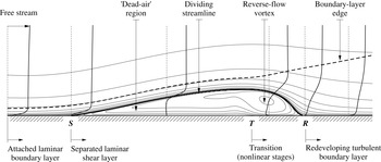
The general structure of a time-averaged separation bubble is presented in figure 1. Figure 1 is an adaptation of a schematic presented by Horton (Reference Horton1968). As a result of the APG and the viscous stresses, fluid particles in the near-wall region of the attached laminar boundary layer slow down until the velocity profile becomes inflectional. A separation point,
 $\boldsymbol{S}$
, is typically defined as the first downstream location for which the skin friction vanishes and subsequently assumes negative values. Just downstream of separation, and below the dividing streamline, the fluid is almost stagnant. This region is often referred to as the ‘dead-air’ region. Due to the small velocities in this area, the pressure remains almost constant, which typically results in a pronounced pressure plateau in the wall-pressure distribution. The separated laminar shear layer is characterized by inflectional reverse-flow profiles which support the amplification of small disturbances in the early stages of transition. Farther downstream the shear layer becomes wavy and rolls up into spanwise vortices (often referred to as ‘rollers’), which detach from the shear layer and are convected downstream (vortex shedding). These vortices considerably increase the wall-normal momentum exchange by transporting low-momentum fluid away from the wall and high-momentum free-stream fluid towards the wall. In the time-averaged picture, however, the process of shear-layer roll up and shedding of vortices cannot be seen. The mean velocity profiles in the region of the reverse-flow vortex exhibit the largest reverse-flow magnitudes in the separation bubble. In addition, the disturbance amplitudes are large, which gives rise to three-dimensional (3-D) secondary instabilities and nonlinear wave interactions. Although transition is to be considered a process rather than a local event, it is common to define a ‘transition onset point’,
 $\boldsymbol{T}$
, as, for example, the location of the minimum skin-friction coefficient. The downstream extent of the transition region depends on multiple factors such as the Reynolds numbers, the APG and the disturbance spectrum. Shortly downstream of transition, the flow reattaches due to both entrainment of free-stream fluid and increased wall-normal mixing. The mean reattachment point,
 $\boldsymbol{R}$
, can be defined as the last downstream location for which the (time-mean) skin-friction vanishes and subsequently assumes positive values.
Mean-flow structure of a laminar separation bubble on a flat plate. Plotted are streamlines, selected streamwise velocity profiles as well as the boundary-layer thickness.

1.1 Transition in laminar separation bubbles
The technical relevance of LSBs has motivated a large number of experimental, theoretical and numerical studies of the stability and transition process. Overviews of the subject are given by Rist (Reference Rist1998) and Boiko et al. (Reference Boiko, Grek, Dogval and Kozlov2002). In general, the transition process in wall-bounded external shear flows can be understood as a progression of stages. Morkovin, Reshotko & Herbert (Reference Morkovin, Reshotko and Herbert1994) discriminate between 5 different paths to turbulence depending on the level of external disturbance excitation. Common to all transition scenarios is an initial stage denoted receptivity (Morkovin Reference Morkovin and Wells1969). Receptivity is the process through which controlled and uncontrolled external disturbances (FST, sound, wall blowing and suction, etc.) enter the boundary layer and generate disturbances of certain amplitudes, frequencies and wavenumbers. The resulting disturbance spectrum greatly influences the ensuing transition scenario. For example, the effect of very high levels of FST and the associated forcing of the boundary layer at large amplitude is known to quickly lead to breakdown of the flow prior to separation and suppress the separation bubble completely. Such a transition scenario is often categorized as ‘bypass’ transition (Morkovin Reference Morkovin1979) since linear stages have no influence on the transition process and are bypassed on the route to turbulence.
For very low levels of environmental disturbances (see also Marxen Reference Marxen2005, for a detailed discussion), transition is initiated by the exponential amplification (modal growth) of so-called Tollmien–Schlichting (TS) waves. The inflectional velocity profiles in LSBs give rise to an inviscid instability mechanism (Kelvin–Helmholtz (KH) instability) with large amplification rates.
It is known (from linear stability theory (LST) analysis, for example) that two-dimensional (2-D) disturbances are more amplified than 3-D disturbances in separated shear layers. Therefore, they typically saturate first, leading to the commonly observed periodic shedding of spanwise coherent (2-D) vortices. At this stage secondary mechanisms set in and break the remaining symmetries of the disturbed flow. For examples and discussions of secondary flow instabilities in LSBs the reader is referred to the corresponding literature (Rist Reference Rist1998; Maucher Reference Maucher2000; Embacher Reference Embacher2006; Jones, Sandberg & Sandham Reference Jones, Sandberg and Sandham2008; Marxen, Lang & Rist Reference Marxen, Lang and Rist2013).
For increased levels of free-stream disturbances, transition in LSBs might be preceded by transient growth of steady streamwise disturbances in the favourable pressure-gradient (FPG) region of the flow. Transient growth is associated with the non-normality of the linearized Navier–Stokes operator (see Trefethen et al. Reference Trefethen, Trefethen, Reddy and Driscoll1993; Schmid & Henningson Reference Schmid and Henningson2001, for example). Superposition of individual non-orthogonal eigenmodes can lead to algebraic growth for some downstream distance before exponential decay due to viscosity becomes the overwhelming factor. A physical explanation for transient growth is provided by the so-called ‘lift-up’ effect (Ellingsen & Palm Reference Ellingsen and Palm1975; Landahl Reference Landahl1975).
This mechanism may result in strong streamwise streaks which modulate the boundary layer in the spanwise direction. McAuliffe & Yaras (Reference McAuliffe and Yaras2010) showed that for a ‘short’ LSB under elevated levels of FST (
 $Tu=1.45\,\%$
at separation), the nature of the instability mechanism changes from amplification due to the KH instability to amplification of streamwise streaks. These streaks extend into the region of laminar separated flow and initiate breakdown via the formation of turbulent spots.
In practical situations, disturbances from different paths will likely coexist and interact with each other. Wind tunnel experiments carried out for a flat-plate boundary layer by Kosorygin & Polyakov (Reference Kosorygin and Polyakov1990), for example, show that in the intermediate range of free-stream fluctuations (
 $0.1\,\%<Tu<0.7\,\%$
) both TS waves and streamwise boundary-layer streaks can grow simultaneously. Wu et al. (Reference Wu, Jacobs, Hunt and Durbin1999) and Wu & Durbin (Reference Wu and Durbin2001) employed 3-D direct numerical simulation (DNS) to investigate the separated flow in a low-pressure turbine stage under the influence of turbulent, periodically passing wakes. They studied the connection between classical linear growth mechanisms (TS, KH) and transient growth, concluding that transient growth plays an important role in this context. From recent DNS results (Fasel Reference Fasel2002; Liu, Zaki & Durbin Reference Liu, Zaki and Durbin2008a
,Reference Liu, Zaki and Durbin
b
) emerges a picture of complex interactions between the streamwise streaks and TS waves. While steady streaks may have a stabilizing effect on TS waves, unsteady streaks can enhance secondary instabilities of TS waves and promote transition.
1.2 The effect of free-stream turbulence
The free-stream turbulence intensity (FSTI) can be relatively low for free-flight applications (
 ${<}0.1\,\%$
) and wind tunnel experiments (
 $\simeq 0.7\,\%$
, and lower) (Kurian & Fransson Reference Kurian and Fransson2009), but can also be very high, as in turbomachinery flow. For the latter, FSTI as high as 20 % has been reported (e.g. Hourmouziadis Reference Hourmouziadis2000). Lower FST levels of the order of 10 % have been measured in a LPT environment (Sharma Reference Sharma1998). Whereas in external flows the FST is rather uniform, the turbulence in turbomachinery flow is often concentrated in the airfoil wakes periodically impinging on downstream blade rows.
Historically, FST has made it very difficult to identify linear stages of the transition process. Experimental evidence of TS waves, for example, was not at hand until Schubauer & Skramstad (Reference Schubauer and Skramstad1948) managed to reduce the level of turbulent fluctuations in the free stream to ‘unusually low values’ (
 ${\sim}1\,\%$
). The success of Schubauer’s experiments could in part be attributed to suggestions by Dryden (Reference Dryden1936) who carried out experiments at a much more turbulent free stream. He reported slow irregular
 $u$
-velocity fluctuations of large amplitude in the laminar region of the boundary layer that were induced by the turbulence in the free stream. In fact, transition in wind tunnel experiments typically seems to be preceded by such a low-frequency streaky modulation of the boundary layer. Today, these streaks are commonly referred to as ‘Klebanoff modes’ (
 $K$
-mode) or ‘Klebanoff distortions’ after Klebanoff, who investigated this phenomenon and described them as a periodic thickening/thinning of the boundary layer (Klebanoff & Tidstrom Reference Klebanoff and Tidstrom1959; Klebanoff Reference Klebanoff1971). From other experimental studies investigating the effect of FST, it has been established that in addition to its low frequency and high amplitude,
 $u_{rms}=O(0.1U_{\infty })$
, the Klebanoff mode is also characterized by a distinct spanwise spacing of
 $O(2{\it\delta}_{99}-4{\it\delta}_{99})$
and an algebraic streamwise growth proportional to
 $\sqrt{x}$
(Kendall Reference Kendall1985, Reference Kendall1990; Westin et al.
Reference Westin, Boiko, Klingmann, Kozlov and Alfredsson1994). The fact that the response of the boundary layer to continuous forcing from the free stream appears to be limited to a narrow band of the wavenumber–frequency spectrum as well as a certain disturbance growth mechanism (algebraic, instead of, say, exponential) led Fasel (Reference Fasel2002) to conclude that the receptivity of the boundary layer to free-stream turbulence is distributed, rather than concentrated at the leading edge or at a surface imperfection. The streamwise, algebraic growth of the
 $K$
-mode is associated with the lift-up effect and transient growth mechanism described earlier.
In general, a shear layer adjacent to a wall is resistant to fluctuations impinging from the free stream. The observation that eddies convected by the free stream are quickly damped inside the boundary layer due to the mean shear flow has been described as ‘shear sheltering’ (Hunt & Durbin Reference Hunt and Durbin1999). The boundary layer acts as a low-pass filter, admitting predominantly low-frequency modes to penetrate into the boundary layer (see Jacobs & Durbin Reference Jacobs and Durbin1998). Due to streamwise stretching of the ingested free-stream vorticity and transient growth (Saric, Reed & Kerschen Reference Saric, Reed and Kerschen2002), low-frequency high-amplitude streamwise streaks arise in the boundary layer (
 $K$
-mode). TS waves, on the other hand, have higher frequencies and smaller scales than the energy-bearing long-wavelength disturbances that are typical of FST (and sound). Therefore some kind of coupling or rescaling of the free-stream disturbances is necessary in order to allow for energy transfer to the TS modes. It is known that such a coupling can only occur in flow regions where non-parallel effects are important, such as near the leading edge, a wall hump or flow around the separation point (e.g. Kerschen Reference Kerschen, Reda, Reed and Kobayashi1991). When a highly disturbed free stream introduces finite nonlinear disturbances into the laminar boundary layer, linear instability growth of modal disturbances may be ‘bypassed’. Jacobs & Durbin (Reference Jacobs and Durbin2001) employed 3-D DNS to investigate transition in a zero pressure gradient, flat-plate boundary layer with a FSTI of
 $Tu\sim 3.5\,\%$
. His results indicate that bypass transition might be initiated when a boundary layer that is highly distorted by low-speed streaks has become susceptible to higher-frequency disturbances which now enter the boundary layer from the free stream and trigger secondary instabilities of the low-speed Klebanoff distortions. The feasibility of such a bypass mechanism was later experimentally confirmed by Hernon, Walsh & McEligot (Reference Hernon, Walsh and McEligot2007).
Naturally, the effect of FST is equally important in the presence of streamwise pressure gradients and the formation of a laminar separation bubble (Mayle Reference Mayle1991). Elevated levels of FST have been reported to reduce the length of the separation bubble (Gault Reference Gault1955; Volino Reference Volino2002; Lardeau, Leschziner & Zaki Reference Lardeau, Leschziner and Zaki2012) or even prevent separation completely by transitioning the flow upstream of the separation location (Dong & Cumpsty Reference Dong and Cumpsty1990; Zaki, Wissink & Durbin Reference Zaki, Wissink, Rodi and Durbin2010). However, early transition is not necessarily beneficial. The significant increase in skin friction and heat-transfer rate associated with turbulent flow can have a detrimental effect on performance and hardware durability (Sohn & Reshotko Reference Sohn and Reshotko1991).
The existence of low-frequency large-amplitude streaks in the boundary layer and in the separated shear layer has been confirmed in the experiments of Häggmark (Reference Häggmark2000) and Volino (Reference Volino2002). In the experiments by Häggmark (Reference Häggmark2000), LSBs on a flat plate were investigated with low noise and disturbance level (
 $Tu=0.02\,\%$
), and with grid-generated turbulence of 1.5 % intensity. Häggmark (Reference Häggmark2000) reports that there is no strong evidence of 2-D waves in the separated shear layer at
 $Tu=1.5\,\%$
. In addition, he performed a spectral analysis and observed that lower frequencies are dominant in the case of increased FST. Volino’s (2002) experimental investigations focused on the effect of low and high FST levels on the suction side separation of a low-pressure turbine blade. For a low Reynolds number,
 $Re=25\,000$
, he reported that even in the case of high levels of FST (
 $Tu=9\,\%$
), breakdown to turbulence occurred in the separated shear layer above the wall and that the flow did not reattach upstream of the trailing edge. The present work investigates the transition process in a laminar separation bubble developing on a flat plate with strong favourable-to-adverse pressure gradient. Experimental reference data for this configuration are available for comparison. First, a numerical model for realistic, isotropic free-stream turbulence is introduced for the numerical simulations. The model is then applied for investigating the effect of FST on transition and separation for the flat-plate LSB. The main focus is directed towards identifying which hydrodynamic instability mechanisms play a dominant role during the transition process as levels of FST increase.
2 Governing equations
For the present investigation, the 3-D, incompressible, time-dependent Navier–Stokes (NS) equations are solved:
 $$\begin{eqnarray}\displaystyle & \boldsymbol{{\rm\nabla}}\boldsymbol{\cdot }\boldsymbol{v}=0, & \displaystyle\end{eqnarray}$$
 $$\begin{eqnarray}\displaystyle & \displaystyle \frac{\partial \boldsymbol{v}}{\partial t}+(\boldsymbol{v}\boldsymbol{\cdot }\boldsymbol{{\rm\nabla}})\boldsymbol{v}=-\boldsymbol{{\rm\nabla}}p+\frac{1}{Re}{\rm\nabla}^{2}\boldsymbol{v}. & \displaystyle\end{eqnarray}$$
 $L_{\infty }$
, and a reference velocity,
 $U_{\infty }$
,
 $$\begin{eqnarray}\boldsymbol{x}=L_{\infty }\boldsymbol{x}^{\ast },\quad t=\frac{t^{\ast }U_{\infty }}{L_{\infty }},\quad \boldsymbol{v}=\frac{\boldsymbol{v}^{\ast }}{U_{\infty }},\quad p=\frac{p^{\ast }-p_{\infty }^{\ast }}{{\it\rho}U_{\infty }^{2}},\end{eqnarray}$$
where dimensional quantities are denoted by an asterisk and
 $p_{\infty }^{\ast }$
is the pressure at some convenient reference point in the fluid. The Reynolds number in (2.1a
) is defined as
 $Re=L_{\infty }U_{\infty }/{\it\nu}$
where
 ${\it\nu}$
is the kinematic viscosity.
Depending on the application and geometry, numerous numerical methods to solve the incompressible NS equations have been developed and employed over the past decades. Although most of these methods are based on primitive-variable approaches (solving for
 $\boldsymbol{v}$
and
 $p$
), none has emerged as an universal approach. Difficulties in defining non-ambiguous boundary conditions for pressure have led to alternative formulations in which pressure as a dependent variable is eliminated. One such alternative, employed in the present investigation, is the vorticity–velocity formulation, which is obtained by taking the curl of the momentum equation (2.1a
) and taking into consideration the fact that both velocity and vorticity vectors are solenoidal. With the definition of vorticity as the negative curl of the velocity vector,
 ${\bf\omega}=-\boldsymbol{{\rm\nabla}}\times \boldsymbol{v}$
, the set of governing equation in vorticity–velocity formulation can be derived,
 $$\begin{eqnarray}\displaystyle & \displaystyle \frac{\partial {\bf\omega}}{\partial t}+(\boldsymbol{v}\boldsymbol{\cdot }\boldsymbol{{\rm\nabla}}){\bf\omega}=({\bf\omega}\boldsymbol{\cdot }\boldsymbol{{\rm\nabla}})\boldsymbol{v}+\frac{1}{Re}{\rm\nabla}^{2}{\bf\omega}, & \displaystyle\end{eqnarray}$$
 $$\begin{eqnarray}\displaystyle & {\rm\nabla}^{2}\boldsymbol{v}=\boldsymbol{{\rm\nabla}}\times {\bf\omega}. & \displaystyle\end{eqnarray}$$
3 Numerical method
Numerical solutions to the governing equations are obtained by employing a Cartesian NS solver first developed by Meitz (Reference Meitz1996). Improvements to the solver, in particular the parallel algorithm, were contributed by Postl (Reference Postl2005) and Balzer (Reference Balzer2011). The code has been thoroughly validated and employed successfully for numerous investigations of transitional and turbulent shear flows, in particular boundary-layer transition (Meitz & Fasel Reference Meitz and Fasel2000; Fasel Reference Fasel2002), laminar and turbulent separation bubbles (Fasel & Postl Reference Fasel and Postl2006; Postl & Fasel Reference Postl and Fasel2006) as well as separation control using vortex generator jets (Postl, Balzer & Fasel Reference Postl, Balzer and Fasel2011).
The numerical solution of the governing equations is advanced in time using an explicit, fourth-order accurate Runge–Kutta method (see Ferziger Reference Ferziger1998, for example). The spatial derivatives in the streamwise (
 $\partial ^{i}/\partial x^{i}$
) and in the wall-normal (
 $\partial ^{i}/\partial y^{i}$
) directions are discretized using fourth-order accurate compact differences (Lele Reference Lele1992). An exception are the streamwise first derivatives of the nonlinear terms, which are discretized using fourth-order accurate split compact differences resulting in improved stability characteristics compared to standard compact differences. Most computational time is expended for obtaining the solution of the wall-normal velocity component, which is governed by a Poisson equation. A solution is obtained by a direct method using standard compact differences and Fourier sine transforms.
Since the flow is assumed to be periodic in the spanwise direction,
 $z$
, periodic boundary conditions are applied for all variables and their derivatives. Each variable is represented by a total of
 $2K+1$
Fourier modes. Fast Fourier transforms (FFTs) are employed to convert each variable from spectral space to physical space and back.
At the upper boundary, a Dirichlet condition is used for the wall-normal velocity to emulate the free-stream acceleration and deceleration associated with the displacement body employed in the experiments. In addition, irrotational flow is assumed,
 ${\bf\omega}=0$
. Since the equations for the streamwise (
 $u$
) and spanwise (
 $w$
) velocity components reduce to ordinary differential equations in the streamwise direction, no free-stream boundary conditions are required for these variables. At the wall, no-slip and no-penetration conditions are imposed.
At the inflow boundary,
 $x=x_{0}$
, all velocity and vorticity components are prescribed as Dirichlet conditions. For maintaining the fourth-order accuracy of the code, the streamwise derivatives are prescribed as well. To prevent reflections from the outflow boundary, turbulent fluctuations are damped out in a buffer domain using the approach proposed by Meitz & Fasel (Reference Meitz and Fasel2000).
A 2-D, steady, laminar base flow solution serves as initial solution. For simulating realistic, free-stream turbulent inflow conditions, an unsteady disturbance field is imposed onto the steady, undisturbed base flow profile:
 $$\begin{eqnarray}\displaystyle [U^{k},V^{k},W^{k}]^{\text{T}}(x_{0},y,t) & = & \displaystyle \left\{\begin{array}{@{}ll@{}}[U_{B},V_{B},0]^{\text{T}}(x_{0},y)+[u^{\prime k},v^{\prime k},w^{\prime k}]^{\text{T}}(x_{0},y,t)\quad & k=0\\ \text{}[u^{\prime k},v^{\prime k},w^{\prime k}]^{\text{T}}(x_{0},y,t)\quad & \forall k\neq 0,\end{array}\right.\end{eqnarray}$$
 $$\begin{eqnarray}\displaystyle [{\it\Omega}_{x}^{k},{\it\Omega}_{y}^{k},{\it\Omega}_{z}^{k}]^{\text{T}}(x_{0},y,t) & = & \displaystyle \left\{\begin{array}{@{}ll@{}}[0,0,{\it\Omega}_{z,B}]^{\text{T}}(x_{0},y)+[{\it\omega}_{x}^{\prime k},{\it\omega}_{y}^{\prime k},{\it\omega}_{z}^{\prime k}]^{\text{T}}(x_{0},y,t)\quad & k=0\\ \text{}[{\it\omega}_{x}^{\prime k},{\it\omega}_{y}^{\prime k},{\it\omega}_{z}^{\prime k}]^{\text{T}}(x_{0},y,t)\quad & \forall k\neq 0.\end{array}\right.\qquad\end{eqnarray}$$
4 A numerical model of free-stream turbulence
For the generation of realistic free-stream disturbance fields, the method of Jacobs & Durbin (Reference Jacobs and Durbin2001) was adopted and implemented in the present Navier–Stokes code. In this approach, turbulent fluctuations are introduced at the inflow boundary plane
 $(x_{0},y,z)$
of the computational domain. These fluctuations are modelled as random velocity and vorticity disturbances which are designed to satisfy continuity, and represent isotropic turbulence with a specified energy spectrum. The method is based on an expansion of the disturbance velocity,
 $\boldsymbol{v}^{\prime }$
, in terms of its Fourier coefficients,
 $$\begin{eqnarray}\boldsymbol{v}^{\prime }(x_{0},y,z,t)=\mathop{\sum }_{{\it\beta}}\mathop{\sum }_{k_{z}}\mathop{\sum }_{k_{y}}A(|\boldsymbol{k}|)\unicode[STIX]{x1D731}(y;{\it\beta},k_{z},k_{y})\text{e}^{\text{i}k_{z}z}\text{e}^{-\text{i}{\it\omega}t},\end{eqnarray}$$
where the dispersion relation
 $k_{x}={\it\beta}/U_{\infty }$
was used to express the streamwise wavenumber in terms of the frequency,
 ${\it\beta}$
. Furthermore, the expansion in wall-normal direction is carried out using superpositions of local solutions from the continuous spectrum of the Orr–Sommerfeld and the Squire operator,
 $\unicode[STIX]{x1D731}$
. Jacobs & Durbin (Reference Jacobs and Durbin2001) recognized that the continuous modes are ideally suitable for the generation of inflow disturbances in the presence of a wall since they are sinusoidal in the free stream but naturally decay inside the boundary layer to low amplitudes. The complete inflow boundary condition is a superposition of a steady, undisturbed base flow
 $\boldsymbol{V}_{B}$
(e.g. a Blasius boundary-layer profile) and the unsteady disturbance velocity:
 $$\begin{eqnarray}\boldsymbol{V}(x_{0},y,z,t)=\boldsymbol{V}_{B}(y)+\boldsymbol{v}^{\prime }(x_{0},y,z,t).\end{eqnarray}$$
In the same manner, the inflow boundary condition for the vorticity field becomes
 $$\begin{eqnarray}{\it\bf\Omega}(x_{0},y,z,t)={\it\bf\Omega}_{B}(y)+{\bf\omega}^{\prime }(x_{0},y,z,t),\end{eqnarray}$$
where
 ${\bf\omega}^{\prime }$
is determined from the disturbance velocity field as
 ${\bf\omega}^{\prime }=-\boldsymbol{{\rm\nabla}}\times \boldsymbol{v}^{\prime }$
.
The expansion coefficients,
 $A(|\boldsymbol{k}|)$
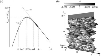
, can be used to distribute turbulent kinetic energy among the disturbance modes. A common choice for the analytic form of the energy spectrum is the von Kármán spectrum (see figure 2
a). For large scales (small
 $k$
) the spectrum is asymptotically proportional to
 $k^{4}$
. For small scales (large
 $k$
) it approaches Kolmogorov’s (
 $-5/3$
)-law. It can be deduced that the choice of turbulent integral length scale,
 $L_{11}$
, controls the size (wavenumber) of the most energetic structures (
 $k_{max}\approx 1.157L_{11}$
) while the turbulent intensity,
 $Tu$
, controls the amplitude levels of these disturbances.
(a) Typical von Kármán energy spectrum (——). The symbols (○) mark the range of wavenumbers realized in a numerical simulation. (b) Instantaneous elevated-surface plot of the spanwise disturbance velocity,
 $w^{\prime }$
, used for introducing FST in the presented simulations. The edge of the boundary layer of the undisturbed flow is indicated by the boundary layer thickness,
 ${\it\delta}_{99}$
.

Upon choosing the parameters
 $L_{11}$
and
 $Tu$
, the inflow velocity and vorticity fields can be completely determined. Figure 2(b) presents an elevated-surface plot with amplitudes and grey scale based on the instantaneous spanwise disturbance velocity,
 $w^{\prime }$
. This figure emphasizes that the current method only introduces disturbances in the free stream, but leaves the inside of the boundary layer almost undisturbed. Note that the disturbance field plotted in figure 2 also vanishes near the free-stream boundary. It was found that high disturbance levels close to
 $y_{max}$
can lead to numerical instabilities. A smooth ramping function corresponding to an exponential decay was multiplied to each wall-normal eigenfunction before being used for the expansion of the disturbance field.
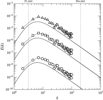
For the present study a total of 1200 continuous modes were used for generation of the inflow disturbance field. Figure 3 presents the theoretical and discrete energy spectrum
 $E(k)$
for all presented cases with
 $Tu\neq 0$
. The turbulent kinetic energy,
 $q^{2}/2$
, is obtained by integrating over the entire 3-D energy spectrum. Energy values for the discrete spectrum are larger than the theoretical values, which results from the condition that both curves should have the same turbulent kinetic energy, i.e.
 $$\begin{eqnarray}\frac{q^{2}}{2}=\int _{0}^{\infty }E(k)\,\text{d}k\approx \mathop{\sum }_{\boldsymbol{k}}E(|\boldsymbol{k}|){\rm\Delta}\boldsymbol{k}.\end{eqnarray}$$
The smallest and largest spanwise wavenumbers which are resolved by the DNS (
 ${\it\gamma}_{1,\mathit{DNS}}$
and
 ${\it\gamma}_{64,\mathit{DNS}}$
, respectively) are indicated by vertical dotted lines in figure 3. Note that for all simulations the free-stream disturbance distribution is the same while the amplitudes/energy increase with increasing levels of free-stream turbulence. Further details of the method, solver implementation, as well as a thorough validation are given in Balzer (Reference Balzer2011).
Spectral kinetic energy spectrum. The lines show the theoretical curve (von Kármán energy spectrum) and symbols correspond to the wavenumbers resolved in the numerical simulation. (○) case FST-0.05; (▫) case FST-0.5; (▵) case FST-2.5.

5 Simulation set-up
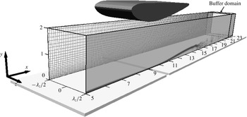
The present computational set-up for the DNS of a flat-plate LSB was motivated by the wind tunnel experiments of Gaster (Reference Gaster1966). The computational domain and grid for these numerical simulations can be seen in figure 4. In the experiments, an inverted airfoil was mounted above a flat plate to accelerate and decelerate the flow between the airfoil and the flat plate. Because circulation control was applied on the airfoil, flow separation and reattachment occurred on the flat plate. This is illustrated in figure 4 by plotting instantaneous grey-scale contours of the spanwise-averaged
 ${\it\omega}_{z}$
-vorticity component.
Simulation set-up motivated by the experiments of Gaster (Reference Gaster1966). For the computational grid, every tenth grid line is shown in both the streamwise and wall-normal direction. Also shown are instantaneous grey-scale contours of the spanwise-averaged
 ${\it\omega}_{z}$
-vorticity component.

Also shown in figure 4 is the computational grid. In the streamwise direction the baseline grid had 2001 equidistantly distributed points in the range
 $5.0\leqslant x\leqslant 23.0$
. The height of the domain was
 $y_{max}=2.0$
(
 ${\approx}19{\it\delta}_{99,0}$
) and exponential grid stretching was employed in the wall-normal direction using 256 grid points. At the solid wall,
 $y=0$
, no-slip and no-penetration boundary conditions were applied. The spanwise domain width was chosen as
 $L_{z}=2.0$
(
 ${\approx}19{\it\delta}_{99,0}$
) and was resolved using
 $K=64$
Fourier cosine and
 $K=64$
Fourier sine modes. The number of collocation points was
 $\mathscr{K}=200$
. The total number of grid points for these simulations was approximately 102 million.
One case was computed with a finer grid (207 million points) in order to demonstrate grid convergence. The refined grid had 2161 and 320 grid points in the streamwise and wall-normal directions, respectively. For the spectral discretization a total of
 $2K+1=193$
Fourier modes was employed using
 $\mathscr{K}=300$
collocation points. Results obtained with the fine grid will be presented and compared to the results obtained with the regular grid.
By variation of the tunnel speed, Gaster (Reference Gaster1966) generated a series of short and long separation bubbles. The present investigation focuses on a long bubble (Gaster’s case VI, series I). The velocity scale was chosen according to the tunnel speed in the experiment,
 $U_{\infty }=6.64$
(
 $\text{m}~\text{s}^{-1}$
), and the reference length scale was
 $L_{\infty }=1~\text{(in.)}=0.0254~\text{(m)}$
. This length scale was chosen because the experimental data were reported in inches. It is, however, not a scale with physical meaning. Marxen (Reference Marxen2005) addressed the question of relevant scales for LSBs developing on a flat plate beneath a displacement body (e.g. 2-D wing section). He pointed out that there exist two, independent length scales (and consequently two relevant Reynolds numbers). The first scale is associated with the distance of the displacement body from the leading edge of the flat plate. In a numerical simulation, the integration domain does typically not include the leading edge. Rather at some location upstream of the displacement body/pressure gradient, an inflow profile is prescribed that matches important boundary-layer parameters (
 ${\it\delta}_{99}$
,
 ${\it\delta}_{1}$
, etc.) of the approach flow. In other words, the distance of the displacement body from the leading edge determines the local boundary-layer properties. In the present numerical set-up, for example, a Blasius similarity solution is prescribed at the inflow,
 $x_{0}=5.0$
, with
 ${\it\delta}_{1}\approx 0.036$
. The corresponding local Reynolds number based on displacement thickness is
 $Re_{{\it\delta}_{1}}=405$
. From Gaster’s (Reference Gaster1966) experiments, only some values at the separation location are known. Here, the boundary-layer edge velocity and Reynolds number based on momentum thickness were
 $u_{e,S}=1.30$
and
 $Re_{{\it\delta}_{2},S}=218$
. In the DNS, these values are
 $u_{e,S}=1.32$
and
 $Re_{{\it\delta}_{2},S}=189$
, respectively, which compare favourably to the values measured in the experiments. The second relevant length scale is associated with the streamwise dimension of the displacement body. The Reynolds number based on this length scale can be related to the pressure gradient. The chord length of the wing section in the experiments was
 $C_{x}=5.5~\text{(in.)}$
and the global Reynolds number based on
 $C_{x}$
was
 $Re\approx 62\,000$
.
For the numerical simulation, the displacement body is replaced with a free-stream boundary condition that imposes a favourable-to-adverse pressure gradient on the mean flow similar to the experiments. The streamwise pressure gradient was enforced by prescribing wall-normal blowing and suction at the free-stream boundary,
 $y_{max}$
. The free-stream
 $v$
-velocity distribution was found iteratively. In similar flat-plate studies (see Lardeau et al.
Reference Lardeau, Leschziner and Zaki2012; Rao et al.
Reference Rao, Jefferson-Loveday, Tucker and Lardeau2014, for example) the geometry of the upper domain boundary is often defined as a streamline such that a free-slip boundary condition can be enforced. Unless this streamline is located sufficiently far away from the wall, however, this approach does not account for the fact that at elevated levels of free-stream turbulence the separation bubble decreases in size resulting in an adjustment of the free-stream streamlines.
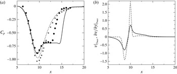
A comparison of the inviscid and viscous wall-pressure coefficient as well as the free-stream distributions for
 $\partial v/\partial y$
and
 $v$
are presented in figure 5. The differences in the inviscid pressure coefficient can be explained by displacement effects of the (tripped) attached turbulent boundary layer in the experiments. For the separated flow, the accelerated flow region and onset of separation (pressure plateau) agree very well between DNS and experiment.
(a) Time- and spanwise-averaged wall-pressure coefficient: (——) 3-D DNS; (– – –) inviscid solution; (●) experiment separated; (
 $+$
) experiment tripped to turbulence. (b) Boundary condition prescribed at
 $y_{max}$
: (——)
 $v$
-velocity distribution for 3-D DNS; (– – –)
 $\partial v/\partial y$
-distribution from inviscid solver.

Despite the good agreement for the upstream part of the bubble, the DNS data indicate later reattachment compared to case VI of the experiments. In fact, it proved very difficult with the current iterative procedure to find a free-stream boundary condition which would yield a shorter bubble without sacrificing the reasonable agreement in the upstream, laminar portion of the flow. From experience it is known that a better comparison can be achieved when some background noise is introduced in the DNS. Therefore, instead of further trying to adjust the free-stream boundary condition, it was decided to apply the numerical FST model for the present case. Employing the FST model was preferred over traditional methods based on introducing selective or random disturbances inside the boundary layer, since it is less artificial and is rather based on relevant physical mechanisms. Note that the choice of a particular inflow profile (Blasius, Falkner–Skan) can also have a significant impact on the developing separated flow. The influence of the inflow profile was, however, not investigated in more detail.
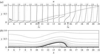
Time- and spanwise-averaged streamwise velocity profiles as well as streamlines are presented in figure 6. Also plotted is the distribution of the boundary-layer thickness. For
 $x<9.5$
,
 ${\it\delta}_{99}$
decreases, which indicates the strong acceleration of the flow upstream of the separation location,
 $x_{S}=10.4$
. In the region of APG, the flow separates and reattaches as a turbulent flow in the mean at
 $x_{R}=15.54$
. The strong growth of the boundary-layer thickness and the full velocity profiles suggest that the flow indeed transitions to turbulence.
Time- and spanwise-averaged results of the uncontrolled separation bubble. (a) Streamwise velocity profiles. The dashed line indicates the boundary-layer thickness,
 ${\it\delta}_{99}$
. (b) Streamlines plotted as equidistant contours of
 $\ln (|10^{4}{\it\psi}|+1)$
. Note that only half of the domain in
 $y$
-direction is shown and that the
 $y$
-direction is scaled by a factor of 3.

In his experiments, Gaster (Reference Gaster1966) reported levels of turbulent free-stream fluctuations of the order of
 $Tu=0.05\,\%$
. For the current flow, six different cases were considered.
-
(1) Case FST-0: ‘quiet’ case; no fluctuations in the free stream;
 $Tu=0$
.
-
(2) Case FST-0.05: low FST level;
$Tu=0.05\,\%$
. -
(3) Case FST-0.5: medium FST level;
$Tu=0.5\,\%$
. -
(4) Case FST-2.5: high FST level;
$Tu=2.5\,\%$
. -
(5) Case FST-2.5b:
$Tu=2.5\,\%$
; DNS are computed on the fine grid. -
(6) Case ZPG-2.5:
$Tu=2.5\,\%$
; DNS are computed without pressure gradient.


The generation of the inflow disturbance field for cases with
 $Tu\neq 0$
was presented in § 4. Comparisons between cases FST-2.5 and FST-2.5b will demonstrate grid convergence. Case ZPG-2.5 serves as a reference case to isolate effects that are associated with the strong favourable-to-adverse streamwise pressure gradient. While the FST intensity is varied, the turbulent integral length scale remains constant and was chosen as
 $L_{11}=5{\it\delta}_{1,0}$
. This is of the order of the values typically used in related investigations of FST-induced transition for attached boundary layers (see Brandt, Schlatter & Henningson Reference Brandt, Schlatter and Henningson2004, for example). It is, however, well known that a change in integral length scale can have a significant impact on the transition location and transition mechanisms (Jonáš, Mazur & Uruba Reference Jonáš, Mazur and Uruba2000; Brandt et al.
Reference Brandt, Schlatter and Henningson2004; Ovchinnikov, Choudhari & Piomelli Reference Ovchinnikov, Choudhari and Piomelli2008). In experiments it is, in fact, rather difficult to vary the turbulence intensity while maintaining the same turbulent characteristic length scales or vice versa (e.g Kurian & Fransson Reference Kurian and Fransson2009). Since the effect of varying turbulent length scales was neglected during the present numerical campaign, the results by no means claim to offer a complete description of the problem.
6 Instantaneous flow
For the purpose of illustration, a modified spanwise vorticity,
 $\breve{{\it\omega}}_{z}$
, is defined as
 $$\begin{eqnarray}\breve{{\it\omega}}_{z}=\ln |{\it\omega}_{z}|.\end{eqnarray}$$
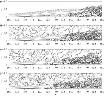
Instantaneous contours of
 $\breve{{\it\omega}}_{z}$
-vorticity are presented in figure 7. The use of a logarithmic scale demonstrates that upstream of transition, two different flow regions can be identified for all cases: (i) an outer region of turbulent fluctuations (except in case FST-0) and (ii) an inner region of the laminar, separated boundary layer. As expected, the mean shear of the boundary layer appears to dampen the high-frequency, vortical disturbances from the free stream (Hunt & Durbin Reference Hunt and Durbin1999).
Contours of spanwise-averaged modified spanwise vorticity,
 $\breve{{\it\omega}}_{z}$
(see (6.1)). Plotted are contour levels
 $-10\leqslant \breve{{\it\omega}}_{z}\leqslant 10$
for DNS with various levels of free-stream turbulent intensity
 $Tu$
. From (a) to (d): case FST-0; case FST-0.05; case FST-0.5; case FST-2.5. Dashed contour lines correspond to
 $\breve{{\it\omega}}_{z}<1$
.

The onset of transition is moved upstream when the level of FST increases. This, in turn, leads to a reduction of the separated flow region. Note that even for the highest FSTI (case FST-2.5), the flow separates from the surface as a laminar boundary layer and transition occurs in the separated shear layer above the surface. While the shear layer still exhibits traces of the roll up and the formation of spanwise-oriented vortices, the reattaching turbulent boundary layer does not appear organized by dominant coherent structures.
Free-stream turbulence induces low-frequency
 $u$
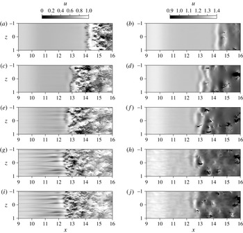
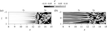
-velocity distortions inside the laminar boundary layer – the so-called Klebanoff modes/distortions. Figure 8 presents instantaneous grey-scale contours of the streamwise velocity component plotted in an
 $x/z$
-plane inside the boundary layer, at
 $y={\it\delta}_{1}(x)$
, and near the edge of the boundary layer, at
 $y={\it\delta}_{99}(x)$
. Values for
 ${\it\delta}_{1}$
and
 ${\it\delta}_{99}$
were obtained from the time- and spanwise-averaged flow fields (see also figure 12). The
 $u$
-velocity contours inside the boundary layer indicate a very sharply defined separation between laminar and turbulent flow regions demonstrating that transition occurs very rapidly over a short streamwise extent. Inside the laminar separated flow region (
 $x<12$
) the flows with non-zero FST are characterized by streamwise-elongated streaks associated with the
 $K$
-mode. These structures are most prominent for case FST-2.5 where they appear with a high amplitude and a distinct spanwise scaling.
Instantaneous grey-scale contours of the streamwise velocity component,
 $u$
, plotted in an
 $x/z$
-plane inside the boundary layer (
 $y={\it\delta}_{1}(x)$
, a,c,e,g,i) and at the edge of the boundary layer (
 $y={\it\delta}_{99}(x)$
, b,d,f,h,j). (a,b) case FST-0, (c,d) case FST-0.05, (e,f) case FST-0.5, (g,h) case FST-2.5 and (i,j) case FST-2.5b.

For the case of very low FST, the Klebanoff distortions have much smaller amplitudes and can only be visualized by looking at the disturbance velocity,
 $u^{\prime }$
, which in this case was calculated by subtracting the spanwise mean from the streamwise velocity, i.e.
 $u^{\prime }=u-U^{0}$
. Grey-scale contours of
 $u^{\prime }$
-velocity are presented in figure 9 for cases FST-0.05 and FST-2.5. Here the local acceleration (
 $u^{\prime }>0$
) and deceleration (
 $u^{\prime }<0$
) that is associated with the
 $K$
-mode can also be seen for the low-level FST case. Nevertheless, in this case the
 $K$
-mode is weak and does not seem to be connected to the turbulent flow region whereas in the case of high FST, the streaks seem to be directly connected to the first-occurring turbulent flow structures in the region
 $12.0<x<13.0$
. Since breakdown of the streaks and/or the appearance of turbulent spots was not observed in any of the present cases, it can be speculated that even for the case with the highest FST intensity, bypass transition can be ruled out as a viable path to turbulence. These results are in agreement with the findings by Lardeau et al. (Reference Lardeau, Leschziner and Zaki2012) who carried out large-eddy simulations for a transitional flat-plate LSB at similar Reynolds number and levels of FST. Isosurfaces of streamwise velocity fluctuations were used to visualize Klebanoff distortions inside the laminar, separated flow region as well as earlier transition onset for cases with increasing FSTIs.
From the flow visualizations in figure 7 and the
 $u$
-velocity contours at
 $y={\it\delta}_{1}$
presented in figure 8 it appears as if the separated shear layer loses its predominantly 2-D character and experiences the onset of flow transition seemingly without the shedding of spanwise vortices. However, the
 $u$
-velocity contours plotted at
 $y={\it\delta}_{99}(x)$
in figure 8 give room for speculation that the reattaching flow might still be organized by such coherent flow structures. For the sake of argument, it is assumed that near the edge of the boundary layer the small-scale turbulence has died out such that the imprint of the large-scale motion can be ‘picked up’. Whereas the grey-scale contours show a strong 2-D spanwise coherence for cases FST-0 (
 $x>14$
) and FST-0.05 (
 $x>13$
), a staggered or ‘checkerboard’ pattern arises for cases FST-0.5 and FST-2.5 (
 $x>12.5$
). A spanwise waviness of the KH vortex followed by earlier transition was also observed by Rao et al. (Reference Rao, Jefferson-Loveday, Tucker and Lardeau2014). The current observation of staggered patterns for the cases with higher levels of FST suggests that slightly oblique waves are more dominant than 2-D waves in these cases. This is often confirmed by carrying out a proper orthogonal decomposition (POD) of the unsteady flow field, which was, however, not attempted for the present cases.
Visualization of the Klebanoff mode for cases FST-0.05 (a) and FST-2.5 (b). Plotted are instantaneous grey-scale contours of the streamwise disturbance velocity component,
 $u^{\prime }=u-U^{0}$
, in an
 $x/z$
-plane at distance
 $y={\it\delta}_{1}(x)$
away from the wall.

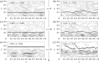
Figure 10 presents an alternative visualization of the streamwise streaks. Here, instantaneous
 $u^{\prime }$
-velocity contours are plotted in three
 $z/y$
-planes for cases FST-0.05 and FST-2.5. The first plane is located in the accelerated flow region at
 $x=8$
. The second plane is located closely upstream of separation at
 $x=10$
, and the third plane is located inside the separated shear-layer region shortly upstream of transition at
 $x=12$
. The thick lines in these plots represent an estimate of the local boundary-layer thickness. For the case with low FST, no significant modulation of the boundary-layer thickness can be seen while for the case with high FST, the high-amplitude streamwise streaks lead to a very pronounced spanwise-periodic thickening and thinning of the boundary layer. The most regular pattern of the
 $K$
-mode is observed at
 $x=10$
where the spanwise streak spacing, measured as the distance between two
 $u^{\prime }$
-velocity minima or maxima, is approximately
 $0.25<{\it\lambda}_{z}<0.35$
. Based on the local boundary-layer thickness, the spacing is of the order of
 $2.5{\it\delta}_{99}-3.5{\it\delta}_{99}$
. A more accurate value will be determined in § 8. Note that the spacing appears to be independent of the intensity of the free-stream fluctuations.
View from upstream. Instantaneous contours of streamwise disturbance velocity,
 $u^{\prime }=u-U^{0}$
, plotted in
 $z/y$
-planes at
 $x=8,10,12$
(from (a,b) to (e,f)). Dashed contour lines indicate negative
 $u^{\prime }$
-values. The thick line represents an estimate of the local boundary-layer thickness. (a,c,e): case FST-0.05; (b,d,f): case FST-2.5.

7 Time- and spanwise-averaged results
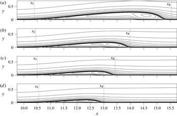
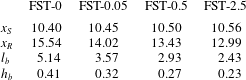
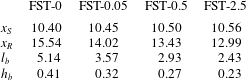
The instantaneous flow visualizations presented in the previous section indicate a reduction of the separation region for increased levels of FST. Time- and spanwise-averaged results of the different flow scenarios are compared in this section to quantify this observation. Streamlines are presented in figure 11. They show a significant reduction in bubble length and height for increasing FST levels, which is confirmed by the mean locations for separation and reattachment as well as bubble length and height listed in table 1. The bubble length is defined as
 $x_{S}-x_{R}$
whereas the bubble height is defined as the boundary-layer thickness,
 ${\it\delta}_{99}$
at the location of maximum displacement thickness,
 ${\it\delta}_{1}$
(see also figure 12). For the case with the lowest FST level the separation length and height are already significantly reduced by 30.5 % and 22.3 %, respectively. Note that the mean separation location remains almost constant, although a general trend can be observed that separation is slightly delayed for increased FSTIs.
Time- and spanwise-averaged streamlines for the uncontrolled flow with various free-stream turbulence intensities. Plotted are equidistant contours of
 $\ln (|10^{4}\cdot {\it\psi}|+1)$
. From (a) to (d): cases FST-0, FST-0.05, FST-0.5 and FST-2.5. Downstream locations of separation,
 $x_{S}$
, and reattachment,
 $x_{R}$
, are indicated as well.

Time-and spanwise-averaged locations of separation,
 $x_{S}$
, and reattachment,
 $x_{R}$
, as well as bubble length,
 $l_{b}$
, and bubble height,
 $h_{b}$
.
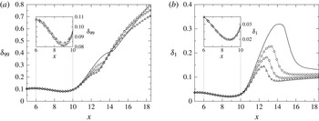
Streamwise distributions of boundary-layer and displacement thickness are presented in figure 12. Prior to separation, the curves are almost identical. Only for the case with 2.5 % FSTI the laminar boundary layer is slightly thicker than for the other cases. Overall, it seems that at the chosen FST levels the boundary-layer fluctuations associated with the
 $K$
-mode have only a local effect but do not significantly alter the time and spanwise mean of the flow field prior to separation. The insensitivity of the mean bubble characteristics with regard to amplitude and type of upstream forcing was also observed by Rist & Augustin (Reference Rist and Augustin2006) who compared the effect of large-amplitude steady 3-D forcing and much weaker 2-D unsteady forcing of a LSB on a flat plate.
Time- and spanwise-averaged boundary-layer thickness (a) and displacement thickness (b) for various levels of FST. (——) case FST-0; (○) case FST-0.05; (▫) case FST-0.5; (▵) case FST-2.5.

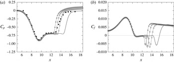
Distributions of wall-pressure and skin-friction coefficients are plotted in figure 13. The agreement with the experimental results for the wall-pressure coefficient is best for
 $0.05\,\%<Tu<0.5\,\%$
. Recall that the FSTI in the experiments was
 $Tu\approx 0.05\,\%$
. The numerical FST model, therefore, proved itself to be very useful for obtaining a more realistic separation bubble size for this case.
Time- and spanwise-averaged wall-pressure coefficient (a) and skin-friction coefficient (b) for various levels of FST. (●) experiment; (——) case FST-0; (○) case FST-0.05; (▫) case FST-0.5; (▵) case FST-2.5.

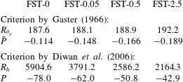
According to Gaster (Reference Gaster1966) the LSB for case FST-0.05 should be considered as ‘long’ bubble since it agrees very well with his experiments (case VI of series I) even if the bubble size was significantly reduced from case FST-0 to case FST-0.05. A clear distinction between ‘short’ and ‘long’ bubbles, a classification introduced by Owen & Klanfer (Reference Owen and Klanfer1953), is quite difficult. From an engineering point of view, it is more intuitive to denote a bubble as ‘short’ if it causes only a small deviation from the inviscid pressure distribution, and as ‘long’ if it alters the pressure distribution completely. The latter is typically found to be detrimental to the aerodynamic performance (of an airfoil, for example). More importantly, the common observation that the transformation from a ‘short’ to a ‘long’ separation bubble can occur suddenly (bubble bursting, see McCullough & Gault Reference McCullough and Gault1951, for example) has motivated the search for a criterion that describes this phenomenon. Gaster (Reference Gaster1966) introduced a non-dimensional pressure-gradient parameter,
 $\bar{P}=({\it\delta}_{2,S}^{2}/{\it\nu})({\rm\Delta}U/{\rm\Delta}x)$
, based on the momentum thickness at separation and the inviscid rise in velocity,
 ${\rm\Delta}U$
, over the length of the bubble,
 ${\rm\Delta}x$
. For ‘long’ bubbles he found a strong correlation between
 $\bar{P}$
and the Reynolds number at separation based on the momentum thickness,
 $Re_{{\it\delta}_{2,S}}$
. For case VI of series I,
 $Re_{{\it\delta}_{2,S}}=218$
and
 $\bar{P}=-0.199$
are reported by Gaster. Due to a slightly thinner boundary layer of the approach flow in the DNS these values are similar but lower compared to the experiment (see table 2).
Parameters for ‘short’ versus ‘long’ bubble criterion by Gaster (Reference Gaster1966) and Diwan, Chetan & Ramesh (Reference Diwan, Chetan and Ramesh2006).
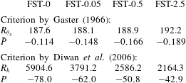
Diwan et al. (Reference Diwan, Chetan and Ramesh2006) propose an alternative criterion that includes also the height of the separation bubble to better capture the global nature of the bubble. They define the non-dimensional pressure-gradient parameter as
 $P=(h^{2}/{\it\nu})({\rm\Delta}U/{\rm\Delta}x)$
and compare it to the Reynolds number based on bubble height and free-stream velocity at that location,
 $Re_{h}$
. The velocity gradient in this criterion is defined as the mean velocity gradient across the length of the bubble rather than the inviscid gradient used by Gaster. Comparing values of
 $P$
and
 $Re_{h}$
for existing data sets, Diwan et al. (Reference Diwan, Chetan and Ramesh2006) identify a critical value of
 $P\approx -28$
. For
 $P>-28$
a bubble is described as ‘short’ otherwise as ‘long’. For all current cases, the calculated pressure-gradient parameters (compiled in table 2) are below the critical value. Both bubble criteria would therefore classify the LSBs of the simulations presented here as ‘long’ even for highest level of FST. It can be speculated, however, that free-stream turbulence does have an effect on bubble bursting, for which both the term and the phenomenon itself are not well understood.
8 Turbulence statistics
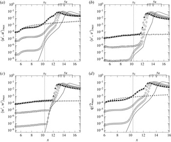
The downstream development of selected spanwise-averaged Reynolds stresses as well as the turbulent kinetic energy,
 $q/2$
, is depicted in figure 14. Plotted are values for the wall-normal maxima inside the boundary layer. Note that especially for high levels of FST, a global disturbance maximum could be located in the free stream rather than near the wall. With increasing FST the disturbance level inside the boundary layer increases as well. Although the fluctuations in the free stream are nearly isotropic, inside the boundary layer
 $\langle v^{\prime },v^{\prime }\rangle$
is approximately one order of magnitude smaller than
 $\langle u^{\prime },u^{\prime }\rangle$
and
 $\langle w^{\prime },w^{\prime }\rangle$
. As indicated by the location of
 $x_{R}$
in figure 14, reattachment of the flow occurs shortly after the disturbance components have reached their maximum amplitudes. The distance between the maximum and
 $x_{R}$
reduces as the FST increases. This could be explained by the fact that for larger FST levels the separation bubble is shallower and that transition occurs closer to the surface such that the turbulent mixing leads to a more rapid and ‘effective’ reattachment of the bubble.
Downstream development of selected spanwise-averaged Reynolds stresses. (a)
 $\langle u^{\prime },u^{\prime }\rangle$
; (b)
 $\langle v^{\prime },v^{\prime }\rangle$
; (c)
 $\langle w^{\prime },w^{\prime }\rangle$
; (d)
 $q/2$
. Plotted are the maximum values inside the boundary layer,
 $y<{\it\delta}_{99}$
. (——) case FST-0; (○) case FST-0.05; (▫) case FST-0.5; (▵) case FST-2.5; (▴) case FST-2.5b; (
 $+$
) case ZPG-2.5. Downstream locations of separation,
 $x_{S}$
, and reattachment,
 $x_{R}$
, are also indicated.

For
 $x<12$
, the
 $\langle u^{\prime },u^{\prime }\rangle$
Reynolds stress component exhibits algebraic streamwise growth which is most likely the consequence of the lift-up mechanism (Ellingsen & Palm Reference Ellingsen and Palm1975; Landahl Reference Landahl1975) and transient growth. Evidence for such a conclusion is provided by the fact that only
 $\langle u^{\prime },u^{\prime }\rangle$
shows this distinct streamwise growth while amplification of the other Reynolds stresses remains rather modest. (Marxen et al. (Reference Marxen, Lang, Rist, Levin and Henningson2009) point out that transient growth acts strongest on those disturbance components that are aligned with the mean flow. Modal growth, on the other hand, is typically characterized by very similar growth rates for all velocity components.) The comparison between case ZPG-2.5 (zero pressure gradient) and FST-2.5 shows that in the region of FPG,
 $x<9$
, transient growth is alleviated. However, in the region of APG and separated mean flow, transient growth appears significantly stronger than for the ZPG case. Using an adjoint-based optimization technique, Levin & Henningson (Reference Levin and Henningson2003) also find increased algebraic growth for optimal disturbances in APG compared to ZPG Falkner–Skan boundary layers. It should be noted that the free-stream disturbances applied in the current DNS study do not force the particular streamwise vortices which represent the optimal disturbances inside the boundary layer that cause the maximum possible algebraic growth. Nevertheless, the introduced disturbance spectrum contains streamwise vorticity which will trigger streamwise streaks, which are observed to grow algebraically albeit at lower than the optimal growth rate.
While the growth rates are almost identical for all cases in the FPG region of the flow field, they are seen to increase in the APG region as the FST level decreases. One explanation for this behaviour could be that the separation bubble grows as FST decreases, which, in turn, might give rise to higher amplification rates. Such a conclusion is corroborated by similar observations for the inviscid KH shear-layer instability, i.e. a longer bubble, possibly with larger distance between the separated shear layer and the adjacent surface, typically gives rise to larger KH growth rates. It is also noted that the onset of
 $v$
-velocity and
 $w$
-velocity disturbance growth commences farther upstream when the level of FST decreases. Another interesting observation is that the strong streamwise growth of
 $\langle v^{\prime },v^{\prime }\rangle$
for case FST-0.05 in the range
 $9.5<x<12$
has no counterpart in the other cases. The growth rates in this flow region are initially identical for the
 $u$
-velocity and the
 $v$
-velocity disturbance. It is not clear at this stage how to interpret these results. On the one hand, it can be speculated that a second instability mechanism (possibly a Görtler-type instability) might exist near the separation point for case FST-0.05. On the other hand, the similarity between the case without any FST (case FST-0) and case FST-0.05 indicates that the behaviour might also be caused by the disturbance equilibrium of the numerical scheme. The disturbance development seen in figure 14 also hints to the fact that transient growth alone does not explain transition to turbulence for the current cases. For
 $x>12$
, the algebraic growth is overtaken by a strong exponential growth equally observed for all Reynolds stress components. In § 10, it will be shown that this growth is, in fact, associated with the KH shear-layer instability.
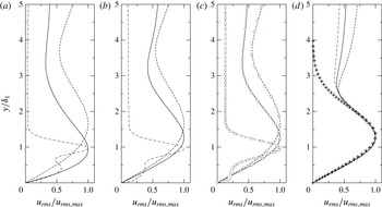
Wall-normal
 $u_{rms}$
-profiles at
 $x=8$
(——),
 $x=10$
(– – –), and
 $x=12$
(– ⋅ – ⋅ –). The profiles are normalized by the local maximum inside the boundary layer. (a) case FST-0.05; (b) case FST-0.5; (c) cases FST-2.5 (lines) and FST-2.5b (○); (d) case ZPG-2.5. Results from optimal disturbance growth theory (Luchini Reference Luchini2000) are also included (
 $+$
).

Wall-normal
 $u_{rms}$
-profiles (
 $u_{rms}=\langle u^{\prime },u^{\prime }\rangle ^{1/2}$
) extracted at
 $x=8,10,12$
are presented in figure 15. The disturbance profiles are normalized by their respective maxima inside the boundary/shear layer and the
 $y$
-direction is normalized by the displacement thickness in these graphs. For the ZPG case (figure 15
d) the profiles are nearly self-similar over a great portion of the boundary layer with a maximum at
 $y/{\it\delta}_{1}\approx 1.3$
. Moreover, the profiles compare very well to the
 $u_{rms}$
-distribution obtained from optimal disturbance growth theory (Luchini Reference Luchini2000, e.g.). It is in fact a common observation in the literature that the shape of the disturbance profile tends to assume the shape of the optimal response even if the initial perturbation is far from that of the optimal disturbance. Recall that in optimal perturbation theory the
 $u$
-velocity streaks are a response to counter-rotating vortices inside the boundary layer, whereas in the DNS the streak formation is triggered by the fluctuations in the free stream. This also explains the discrepancy of the curves for
 $y\rightarrow y_{max}$
. The profiles are not self-similar (with respect to the scaling
 $y/{\it\delta}_{1}$
) for the cases with strong favourable-to-adverse pressure gradient (see figure 15
a–c). However, the similarity of the profile shapes in the attached flow region suggests that the disturbances are caused by the same mechanism (lift-up effect). As the flow separates the maximum of the disturbance aligns with the location of
 ${\it\delta}_{1}$
. Note that this alignment is already completed at
 $x=10$
in the case of low FST (case FST-0.05) while for the other cases it occurs farther downstream. Since the displacement thickness is commensurable with the location of the wall-normal maximum of shear, this shows that the streamwise streaks get ‘pushed up’ as the boundary layer separates and grow within the shear layer.
From hot-wire measurements it is known that the streamwise streaks are strongly correlated in the spanwise direction. The spanwise spacing of the Klebanoff distortions can therefore be assessed by evaluating the spanwise two-point correlation function,
 $R_{uu}$
, of the streamwise velocity:
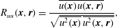 $$\begin{eqnarray}R_{uu}(\boldsymbol{x},\boldsymbol{r})=\frac{\overline{u(\boldsymbol{x})u(\boldsymbol{x},\boldsymbol{r})}}{\sqrt{\overline{u^{2}(\boldsymbol{x})}\;\overline{u^{2}(\boldsymbol{x},\boldsymbol{ r})}}},\end{eqnarray}$$
where the vector separation
 $\boldsymbol{r}$
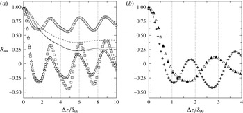
is aligned with the spanwise direction. Figure 16 shows correlations obtained for two
 $y$
-locations: (i) inside and (ii) outside the boundary layer, both plotted at
 $x=10$
. The inner
 $y$
-location corresponds to the wall-normal maximum of the
 $u_{rms}$
-velocity profiles and the outer location corresponds to
 $y=1.5{\it\delta}_{99}$
. The fluctuations in the free stream are uncorrelated while the local
 $R_{uu}$
minima and maxima inside the boundary layer correspond to the alternating nature of the low- and high-momentum flow in the presence of the Klebanoff mode. An interesting observation is that for the case FST-0.05 the correlation distribution assumes much larger values (weaker effect of the
 $K$
-mode) compared to cases FST-0.5 and FST-2.5. However, further upstream, at
 $x=8$
, the distributions were found to be nearly identical for all cases (results not shown). This suggests that the Klebanoff mode becomes less important for the flow distribution inside the separated shear layer in case FST-0.05. Recall that at
 $x=10$
in figure 14 also a different growth of Reynolds stresses between FST-0.05 and the other cases was observed. This could imply that a different physical mechanism has become more relevant than the
 $K$
-mode in this case. Further detailed investigations are necessary to explain the relevant physical basis for these results.
Spanwise two-point correlation function,
 $R_{uu}$
, at
 $x=10$
. Symbols correspond to
 $R_{uu}$
-values inside the boundary layer (max. of
 $u_{rms}$
), and lines correspond to
 $R_{uu}$
-values outside the boundary layer (
 $y=1.5{\it\delta}_{99}$
). (○, – – –) case FST-0.05; (▫, ——) case FST-0.5; (▵, – ⋅ – ⋅ –) case FST-2.5; (▴) case FST-2.5b; (
 $+$
) case ZPG-2.5b.

From flow visualizations (e.g. Kendall Reference Kendall1985) it is known that the spanwise streak spacing is approximately twice the distance to the first minimum in the correlation function. The first minimum is located at
 ${\rm\Delta}z/{\it\delta}_{99}=1.7$
for all cases with non-zero pressure gradient. Therefore the spacing is approximately
 $3.4{\it\delta}_{99}$
, which agrees with the estimate obtained from the
 $u^{\prime }$
-velocity contours presented in figure 10. Note that the fluctuations in the free stream are uncorrelated. Results are also presented for the fine grid and the case of ZPG in figure 16(b). For case ZPG-2.5 the streak spacing is of the order of
 $2{\it\delta}_{99}$
. Note, however, that the boundary layer is approximately 1.6 times thicker at
 $x=10$
in case ZPG-2.5. Thus, the spanwise spacing is almost identical for cases ZPG-2.5 and FST-2.5. This in turn implies that the selection of the spanwise scale is independent of the pressure gradient. Furthermore, the values obtained for the spacing agree well with the distinct spanwise scaling of
 $O(2{\it\delta}_{99}{-}4{\it\delta}_{99})$
reported for ZPG flat-plate boundary layers (Kendall Reference Kendall1985, Reference Kendall1990; Westin et al.
Reference Westin, Boiko, Klingmann, Kozlov and Alfredsson1994). At
 $x=10$
the local ratio of domain width and boundary-layer thickness is
 $L_{z}/{\it\delta}_{99}\approx 21$
. The
 $K$
-mode spacing of
 $3.4{\it\delta}_{99}$
therefore suggests, that approximately 6–7 streaks are resolved in the computational domain. This result agrees with the flow visualizations in figures 8–10.
The excellent agreement between cases FST-2.5 and FST-2.5b in figures 14–16 shows that, in a statistical sense, the numerical solutions are grid independent.
9 Spectral analysis
In order to assess the dynamic behaviour of the separation bubble, time signals of the wall-normal disturbance velocity component,
 $v^{\prime }=v-\bar{v}$
, were analysed to detect dominant frequencies in the flow field. These time signals were taken inside the separated shear layer at the centre of the domain,
 $z=0$
, and at a distance
 $y={\it\delta}_{1}$
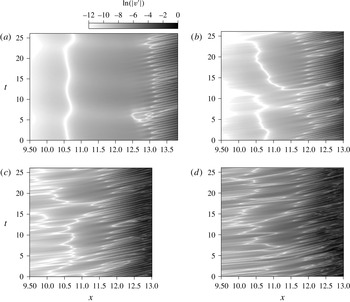
away from the wall. Grey-scale contours of the recorded time signals are presented in figure 17 in form of
 $t/x$
-diagrams. White-coloured contours correspond to regions of vanishing disturbance velocity which, most often, indicate a change of sign of the
 $v^{\prime }$
-velocity. Compared to the case with
 $Tu=0$
, similar dynamic behaviour is observed for the case of low FST (
 $Tu=0.05\,\%$
). Here, the separated shear layer is relatively calm for
 $x<11.5$
followed by the distinct time-periodic pattern associated with vortex shedding. Cases with elevated FST levels show an irregular flow pattern upstream of
 $x=11.5$
. However, farther downstream the same time-periodic behaviour as for the other cases becomes the prominent feature.
Spatio-temporal development of shear-layer disturbances. Plotted are logarithmic grey-scale contours of the wall-normal disturbance velocity component,
 $v^{\prime }$
, at
 $y={\it\delta}_{1}$
and
 $z=0$
. (a) case FST-0; (b) case FST-0.05; (c) case FST-0.5; and (d) case FST-2.5.

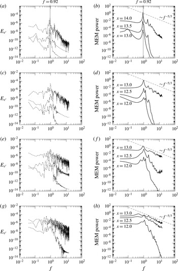
Spectral energy obtained using discrete Fourier transform (DFT, (a,c,e,g)) and maximum entropy method (MEM, (b,d,f,h)) of order
 $M=40$
. (a,b) case FST-0; (c,d) case FST-0.05; (e,f) case FST-0.5; (g,h) case FST-2.5.

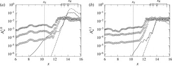
Downstream development of the streamwise disturbance velocity. Plotted are wall-normal maxima of the Fourier amplitude,
 $A_{u}^{1,0}$
(a) and
 $A_{u}^{1,1}$
(b). (——) case FST-0; (– – –) LST of case FST-0; (○) case FST-0.05; (▫) case FST-0.5; (▵) case FST-2.5. Downstream locations of separation,
 $x_{S}$
, and reattachment,
 $x_{R}$
, are indicated as well.

To determine the frequency spectrum associated with these velocity time signals, two spectral methods were employed. First, a discrete Fourier transform (DFT) of the signals was performed, i.e.
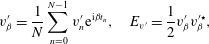 $$\begin{eqnarray}v_{{\it\beta}}^{\prime }=\frac{1}{N}\mathop{\sum }_{n=0}^{N-1}v_{n}^{\prime }\text{e}^{\text{i}{\it\beta}t_{n}},\quad E_{v^{\prime }}=\frac{1}{2}v_{{\it\beta}}^{\prime }v_{{\it\beta}}^{\prime \star },\end{eqnarray}$$
where
 $N$
is the number of samples in the time signal,
 ${\it\beta}=2{\rm\pi}f$
is the circular frequency and
 $E_{v^{\prime }}$
is the spectral energy. Second, a so-called maximum entropy spectral analysis was employed. The maximum entropy method (MEM) has its origin in information theory where it is used for signal processing of data with high levels of broadband noise. MEM estimates the spectral density of a discrete time signal by considering the most random, or least predictable, process that has the same
 $M+1$
autocorrelation coefficients as the given time series, where
 $M$
is called the order of the method (Ghil et al.
Reference Ghil, Allen, Dettinger, Ide, Kondrashov, Mann, Robertson, Saunders, Tian and Varadi2002). The disturbance spectra plotted in figure 18 were generated by performing a DFT and MEM (with
 $M=40$
) for time signals at selected downstream locations. For the flow with
 $Tu=0$
a distinct peak at the fundamental frequency
 $f=0.92$
develops in the streamwise direction. The dimensional frequency is scaled by the reference values for free-stream speed and length scale,
 $f=f^{\ast }L_{\infty }/U_{\infty }$
. Other common scalings for the frequency are based on, for example, the separation bubble length,
 $l_{b}$
. However, as Postl (Reference Postl2005) pointed out,
 $l_{b}$
is not a meaningful length scale for the uncontrolled DNS cases since the low background disturbance levels in the DNS typically result in significantly larger bubbles than in the experiments, where FST and sound disturbances are always present.
As the turbulence in the free stream increases, a dominant frequency, although less pronounced, can still be discerned from these spectra. The value of the frequency increases slightly to
 $f\approx 1.1$
for case FST-2.5. An increase in frequency can be expected, since the size of the separation bubble is reduced for higher FST levels, and, in turn, smaller bubbles promote smaller disturbance wavelengths and higher frequencies. Such a conclusion can be verified by a comparison of LST results for the different mean flows.
The comparison between the DFT and MEM results shows that MEM can be a valuable tool to determine whether preferred frequencies exist in a highly disturbed flow. For case FST-2.5 at
 $x=12.5$
, for example, the time signal is extremely noisy, but MEM is still able to detect the shedding frequency. A comparison with the (
 $-5/3$
)-decay law shows that at
 $x=12.5$
, and especially at
 $x=13.0$
, the inertial subrange is well developed which indicates fully turbulent flow.
10 Inviscid shear-layer instability mechanism
Independent of the FST level, a dominant frequency was found for all cases in the previous section. Moreover, the frequency remained close to the natural shedding frequency of the unforced case FST-0, i.e.
 $f=0.92$
. A dominant peak in the frequency spectrum of separation bubbles can typically be associated with the inviscid shear-layer instability. To confirm this conjecture, DNS and LST results are compared for 2-D and 3-D disturbance waves with the fundamental frequency, in particular Fourier modes
 $(1,0)$
and
 $(1,1)$
. The downstream development of the maximum
 $u^{\prime }$
-velocity Fourier amplitude of these modes, i.e.
 $A_{u}^{1,0}$
and
 $A_{u}^{1,1}$
, is presented in figure 19. Note that
 $A_{u}^{1,0}$
and
 $A_{u}^{1,1}$
represent the maximum inside the boundary/shear layer. As the level of FST increases, the 2-D and 3-D disturbances in the attached laminar boundary layer exhibit higher amplitude levels without experiencing significant downstream growth. This is contrary to the behaviour of the Klebanoff distortions, which were shown to have a distinct growth in the region of attached flow (see figure 14
a). However, farther downstream, inside the separated shear layer, the disturbances grow exponentially until they saturate all at about the same amplitude level (all cases with
 $Tu\neq 0$
). The LST results included in figure 19 for case FST-0 show that the exponential growth of the 2-D and 3-D modes agrees well with linear theory. Note that the LST analysis of all other cases yields similar growth curves, which are omitted in figure 19. For cases FST-0.05, FST-0.5 and FST-2.5, the onset of exponential growth is at
 $x\approx 11.8$
. This is upstream of the location for which disturbances in the unforced case FST-0 exhibit exponential growth,
 $x>12.7$
. Although exponential growth is observed farther upstream for the cases with non-zero FST, it still occurs significantly downstream of the separation location and the location for which LST predicts the onset of exponential growth,
 $x\approx 10$
(not shown in figure 19). This demonstrates that the vortical, turbulent fluctuations in the free stream are not very effective in forcing TS waves with the ‘proper’ frequency. Rather, as shown in § 8, they are responsible for the formation of streamwise streaks.
It is interesting to observe that, for case FST-0, the 2-D mode,
 $(1,0)$
, saturates and remains at amplitude levels of one order of magnitude larger than the 3-D mode,
 $(1,1)$
. This can be seen as an indication for the existence of predominantly 2-D flow structures in the reattaching turbulent flow, which was previously confirmed for similar flows using proper orthogonal decomposition techniques (see Postl et al.
Reference Postl, Balzer and Fasel2011, for example).
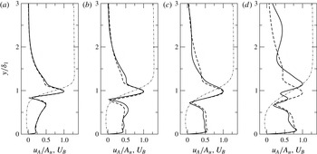
Wall-normal distribution of
 $u^{\prime }$
-velocity Fourier amplitudes obtained from DNS (——) and LST (– – –) for the 2-D mode
 $(1,0)$
. Profiles were extracted at the downstream locations where
 $A_{u}^{1,0}=8\times 10^{-3}$
and scaled by their respective maximum,
 $A_{u}^{1,0}$
. Also shown is the local mean-flow profile,
 $U_{B}$
(– ⋅ – ⋅ –). (a) Case FST-0; (b) case FST-0.05; (c) case FST-0.5; and (d) case FST-2.5.

In all other cases, however, the amplitude levels for the 2-D and 3-D modes are very similar at reattachment and farther downstream. Note, however, that for the Fourier transform all flows were sampled with the same frequency,
 $f=0.92$
. The results might change in favour of the 2-D mode when the sampling is carried out with the slightly higher frequencies that were detected for cases FST-0.05, FST-0.5 and FST-2.5 in § 9.
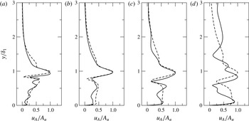
Figures 20 and 21 show wall-normal
 $u^{\prime }$
-velocity Fourier amplitude distributions for modes
 $(1,0)$
and
 $(1,1)$
. These profiles were extracted from the region of exponential growth for which the maxima of the disturbance amplitudes have reached
 $A_{u}^{1,0}=A_{u}^{1,1}=8\times 10^{-3}$
. The shape of the amplitude distributions agrees reasonably well with the
 $u^{\prime }$
-velocity eigenfunctions obtained from LST. Notable differences in the wall-normal location of the disturbance peaks exist for case FST-2.5. It is likely that in this case a second, stable eigenmode with the same frequency but different eigenvalue (streamwise wavenumber and growth rate) was excited (compare figures 11g and 12g in Marxen, Lang & Rist (Reference Marxen, Lang and Rist2012)). Nevertheless, the reasonable agreement between LST and DNS for the region of exponential growth confirms that in all cases both 2-D and weakly oblique 3-D disturbances grow due to the linear, inviscid shear-layer instability mechanism. Therefore, it can be concluded that even for the highest level of FST considered in the present work, the primary linear stage of the transition process is not bypassed. Consequently, unsteady flow control techniques which are aimed at exploiting the shear-layer instability might still be effective means to reduce/eliminate separation in these cases.
Wall-normal distribution of
 $u^{\prime }$
-velocity Fourier amplitudes obtained from DNS (——) and LST (– – –) for the 3-D mode (
 $1,1$
). Profiles were extracted at the downstream locations where
 $A_{u}^{1,1}=8\times 10^{-3}$
and scaled by their respective maximum
 $A_{u}^{1,1}$
. (a) Case FST-0; (b) case FST-0.05; (c) case FST-0.5; and (d) case FST-2.5.

11 Conclusions
A numerical model for realistic FST was employed in order to investigate the effect of FST on separation, in particular on the fundamental hydrodynamic instabilities that are known to govern the transition process for laminar separation bubbles. This was done by prescribing physically meaningful free-stream turbulent velocity and vorticity fields at the inflow boundary. The present work also represents the first attempt to introduce such a model into a Navier–Stokes solver based on the vorticity–velocity formulation.
For the simulations of a separation bubble subject to various levels of FST, a flat-plate model was considered. Elevated FST levels led to the generation of streamwise boundary-layer streaks (Klebanoff modes). The streaks are characterized by a very low frequency, a long streamwise wavelength, and a spanwise spacing of the order of
 $3{\it\delta}_{99}{-}4{\it\delta}_{99}$
. Increasing FST levels caused higher
 $K$
-mode amplitudes inside the boundary layer. In the approach flow, but especially inside the separated flow region, strong algebraic growth of the streaks was observed. At the same time, the presence of the inviscid shear-layer instability was detected for all cases. Thus, for the separation bubble, transition to turbulence was a consequence of both the primary shear-layer instability and the enhanced 3-D disturbance level, in particular the streamwise streaks caused by the FST. Even very small FST levels caused a significant reduction of the size of the separation bubble, which demonstrated that free-stream turbulence can have a significant effect on LSB flows.
Further parameter studies including, for example, the effect of the free-stream turbulent length scales are required to build upon the gained experience and understanding. Nevertheless, the presented results are an important cornerstone in the ongoing effort to emulate physically ever more realistic and challenging flow environments by using numerical simulations.
Acknowledgements
This work was supported by the Air Force Office of Scientific Research (AFOSR) under grant number FA9550-09-1-0214. D. R. Smith served as the program manager. Computer time was provided by the US Army Space and Missile Defense Command (SMDC), the Arctic Region Supercomputing Center (ARSC), as well as the National Center for Computational Sciences (NCCS). We thank S. Hosseinverdi for proofreading the manuscript and his support during final revisions.