II. THEORY OF OPERATION

A driving curiosity that led to the development of our quasi-wireless system was how to transfer power to a load when the circuit return was inaccessible. The main condition being that the distance between the load and return is large and that a counterpoise (large capacitive plate) could not be used. At such distances, the only interconnecting parameter is the stray capacitance (C _STRAY ) which forms a series connection with the load and source. Calculations of the bulk value of C _STRAY are generally of the order of a few picofarads. With such extremely small capacitances, our solution was to use the inductance (L) of the single wire connecting the load (R _L ) to the power supply (V _S ) to form a current (I) in a classic series LRC circuit configuration; where C is the stray capacitance,

(1) $${V_S} = I{R_L} + jI\left( {2\pi \,fL - {{\displaystyle{1 \over {2\pi\, fC}}}_{STRAY}}} \right).$$

Unlike a conventional lumped LRC circuit, the stray capacitance in our system is a distributed element and is proportional to the length and geometry of the wire in combination with the supply. Applying an AC signal at the appropriate frequency places the wire into resonance where the reactive components cancel and the supply sees only the series resistive element (2π fL = 1/2π fC _STRAY ), with active power delivery occurring from the energy dissipated in this resistance. The distributed effect of the C _STRAY forms a special case of resonance where the electrical parameters of each section of the wire are cumulatively added to the next, yet all accumulated sections obtain the same resonant frequency. This causes the voltages and currents to become functions of distance along the wire and produce the classical standing wave pattern [Reference Pain17]. The geometry of the wire generally dictates how well the system is at storing or radiating energy.

The stray capacitance exists as a non-tangible element and is difficult to measure. However, its distribution may be modeled via the accumulative inductance (formulated in [Reference Van Neste16]) with the condition that, at resonance, the reactance of the two elements are equal. The effective perceived $C_{STRAY}^i $ at each turn becomes,

(2) $$C_{STRAY}^i = \displaystyle{1 \over {{\omega ^2}{L_i}}},$$

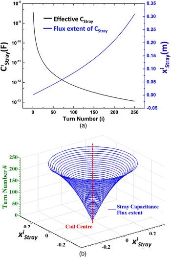
where L _i is the cumulative inductance at each turn (sub/superscript i) and ω = 2πf is the standing wave resonance frequency. The per-turn C _STRAY is plotted in Fig. 1(a) (left). The influence or extent of the stray capacitance flux within the media around the wire that results in the standing wave build-up can be estimated using

(3) $$x_{Stray}^i \approx \left( {\displaystyle{{{a_{wire}}} \over 2}} \right){Q_{frac}}\exp \left[ {\displaystyle{{2\pi {\varepsilon _0}k} \over {C_{Stray}^i /l}}} \right],$$

and is also plotted in Fig. 1(a) (right). Here, $x_{Stray}^i $ is the distance (extent) of stray capacitance projected at the  ith turn of the coil, a _wire being the diameter of the wire, ε₀ the permittivity of free space, k the dielectric constant of the medium around the system, l the circumference of one turn of the coil and Q _frac a non-dimensional factor accounting for the non-uniform distribution of charge. Fig. 1(b) is a three-dimensional (3D) representation that depicts the extent of the stray capacitance envelope, beyond which the standing wave mode is not detuned by external influences. Equation (3) has importance when multiple systems are operated in one area as it defines their relative proximity to each other along with external influences which might affect their resonant conditions.

Fig. 1.

(a) (Left y-axis) Effective stray capacitance as a function of turn number (i), (a) (Right y-axis) the extent of the stray capacitance flux as it extends through the surrounding media. (b) 3D plot of the extent of the stray capacitance flux envelope.

When the system is designed to restrict/suppress radiation, the input energy must experience losses arising from the internal resistance of both the wire and the load, while the energy is reactively exchanged between the stray capacitance and wire inductance each half-cycle. The efficiency of the system is thus defined by the common ratio of load resistance (R _LOAD ) to total resistance (R _TOTAL ) as

(4) $$\eta = \displaystyle{{{R_{LOAD}}} \over {{R_{TOTAL}}}}.$$

The main mechanism of energy transfer therefore becomes the standing wave; which differs significantly from previous WPT systems that rely solely on field coupling or traveling wave mechanics.

Using this standing wave excitation technique, we have previously shown how the active terminal of an AC power supply can be expanded to everyday surfaces with minimal, if any, modification through the operation of static loads (i.e. loads that do not move on their own) [Reference Van Neste16]. We observed a high level of power continuity over the area which led us to investigate its effectiveness at powering mobile loads, as per this study. The superposition of control signals in tandem with power is also possible since energy is able to actively dissipate in the system. This allows us to examine broad area digital signaling to communicate with and control mobile loads without radiating or line-of-sight approaches.

III. EXPERIMENTAL DETAILS

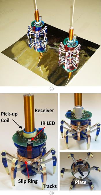
Figure 2(a) shows a photograph of the experimental setup over a metalized polyester sheet. Only one side of the polyester was conductive, with an approximate 50 µm coating of aluminum, while the adjacent side was insulated. To reduce wear and add operational safety, we conducted the experiments on the insulated side of the sheet. Two commercially available Hexbug Spider robots were used for this study. Hexbugs are remote controlled toys with a simple, yet elegant construction. Control of the robots is accomplished through a serial signal output from an infrared (IR) light-emitting diode (LED) located on a remote control, similar to the remote communication found in many televisions.

Fig. 2.

(a) Photograph of two robots used in the study over a metalized polyester sheet acting as the energized surface. (b) Labeled photograph identifying various parts of the robots' modification to accept quasi-wireless surface power.

These robots were constructed almost entirely of plastic and therefore needed to be modified to accept energy from the insulated surface. Using 6.35 mm wide copper-plated tape, tracks were made from the feet of the robot to a central slip-ring where the torso of the robot pivots (Fig. 2(b)). From the slip-ring, a single conductive path continued to a receiver with communication electronics placed at the top of each robot. Both receivers were identical in construction and consisted of 250 turns of 28 gauge magnet wire tightly wrapped around a plastic tube 1.27 cm in diameter and 9 cm long (forming an inductance of 86.45 µH). An additional length of wire 17 cm long was added to the top of each receiver to improve the capacitive coupling with the ground when over a surface. The unloaded standing wave frequency was 10.5 MHz (exhibiting a 40 kHz difference between the pair) with a measured quality factor of 65 for both receivers. To reduce the impedance between the feet and sheet, a 1 in. diameter round foil plate was glued to the bottom of the robots' torso (Fig. 2(a)). The capacitive coupling between the robotic feet/torso and the polyester sheet was measured to be 108 pF.

IV. CIRCUITRY WITH CONTROL

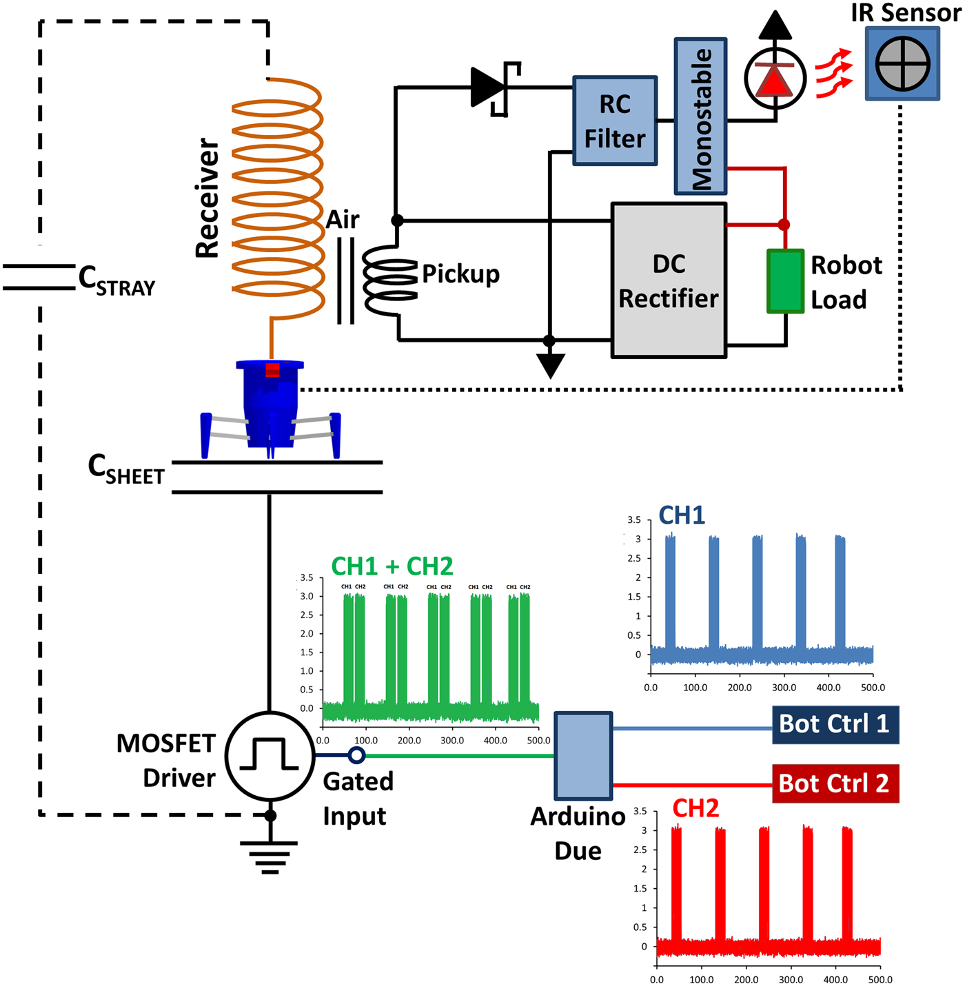
Figure 3 shows a schematic diagram of both the power and control circuitry. While the basic power delivery is similar to our previous work [Reference Van Neste16], here we inductively couple the standing wave energy from the receiver to the load using a pick-up coil composed of 10 turns of 20 gauge wire. The pick-up coil was placed at the location of the current anti-node, which occurs at the bottom of the receiver. The coupling coefficient between the receiver and pickup was 0.6. This creates isolation between the two circuits and allows measurement devices to be connected to the output without altering the standing wave resonance of the system – as measurement devices can, and will, change the system operation when directly connected to the receiver.

Fig. 3.

Schematic diagram of the power and control instrumentation used for the experiment. Each robot control board (labeled Bot Ctrl 1 and 2) was composed of buttons that interfaced with the Arduino Due microcontroller. Each robot was controlled by a set of specific command line sequences that made up a digital channel. Depressing the buttons triggered the C code to output a command line to the gated input of the MOSFET driver. If both control boards were depressed, then the program would properly phase the command lines of each robot, combining the channels sequentially together.

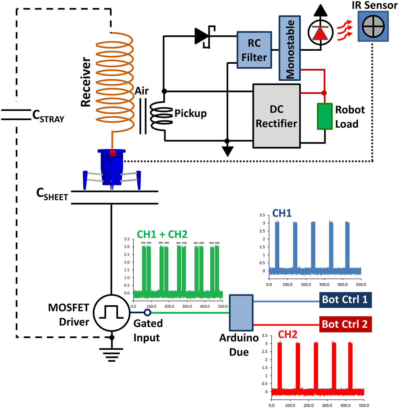
The power to the plate is provided by a MOSFET switching circuit (driver) that generates a square wave output between 0–100 V (70 VRMS) at an adjustable frequency range of 1 Hz to 15 MHz. This is nominally set to 10.5 MHz which is the robots' receiver coil resonant frequency. The 10.5 MHz input to the high-voltage side of the driver is digitally gated with a command sequence to control the robots. A logic zero from the command sequence disrupts the 10.5 MHz to the driver (turning the power signal off) for a short period of time, the length of which has to be longer than the “ring-down” time of the robot's resonator to be detected, but not too long as to have a large effect on the delivered power. The measured ring-down (relaxation) time for both receivers was 365 ns under load.

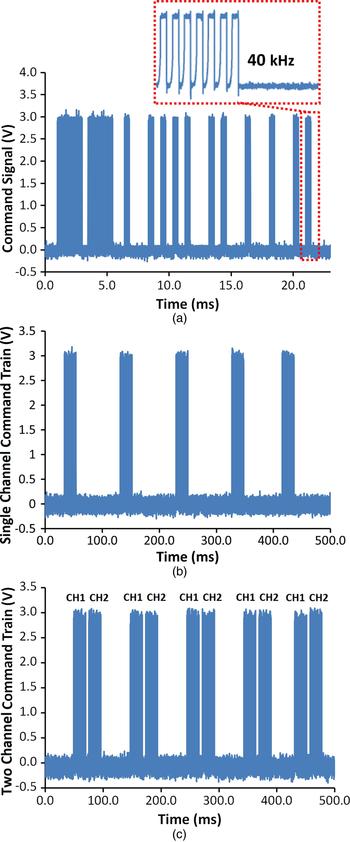
Figure 4(a), along with Fig. 3, shows the typical digital command line used to steer the robots, taken with a Tektronix TDS2024C oscilloscope. Each robot is factory programmed with two separate command channels using a fixed bitrate of 40 kHz (Fig. 3 bottom and Fig. 4(b)). It should be noted that these channels are not physical wire channels, but a combination of digital sequences. When a controller button is depressed, digital bits are sent to the robot that form a command line lasting 20 ms (Fig. 4(a)). These commands are repeated every 77.6 ms that the controller button is held (Fig. 4(b)).

Fig. 4.

(a) Plot of the command line used to control the robot, interlaid at the top is the bitrate which composed each section of the command line. (b) Plot of a signal control “Channel” being defined as the group of command lines used to control a specific robot. Each channel command line was separated by 77.6 ms forming a command train. (c) Plot of the properly phased serial command lines of two channels, each channel output consecutively after the other.

A major challenge encountered was combining the control signals over the surface without the command lines mixing – as this would cause loss of control for both devices. We overcame this obstacle by recording the command train of each channel using an Arduino Due microcontroller board connected to a computer. This allowed us to reproduce the commands in a C programming language environment; allocating the proper position in the time domain for both signals (Fig. 4(c)). The Arduino coding would first identify which of two robots the command was intended and then stack each command line sequentially to produce one contiguous serial command train composed of both channels. The lumped command train would then be sent to the gated input of the MOSFET driver (green waveform at the bottom of Fig. 3, also plotted with better clarity in Fig. 4(c)).

The user interface to produce the control signals was provided by four buttons for each robot (eight buttons total): a–walk forward, b–walk backwards, c–walk sideways (Left), d–walk sideways (Right). Pressing either a or b combined with pressing either c or d gave us eight possible permutations. These permutations were used to produce eight total command sequences per channel; or 16 sequences total. Please note that for confidentiality reasons we are not plotting all command line sequences in this study.

The receiver circuitry of each robot contained a first-order resistor capacitor (RC) filter attached to the pick-up coil in conjunction with a Schottky diode for half-wave rectification (Fig. 3). The rectified RC filter generated a direct current (DC) charge on the capacitor with an applied power signal. If the power signal was briefly modulated to an off state, the capacitor would discharge the DC voltage through the resistor forming an RC time constant. The communication signal was thus created via a short power-break (modulation) over the surface, with each control bit (power off state) detected by the Schmitt trigger of a monostable multivibrator. The triggering of the monostable would occur when the voltage across the capacitor in the rectified RC filter reduced below the monostable's threshold during the off state. The monostable output would then stay low for a set amount of time (12.5 µs, the pulse width of the robots' factory bitrate) upon which it would return to a high state, awaiting another discharge of the filter's capacitor. This created a form of bit compression as the bit pulse width (off-time) over the surface could be much smaller than the required factory default. The monostable output signal was fed to an IR LED directly above the IR sensor of the robot. The close proximity of the LED allowed the LED to function at a low-intensity and conserve power. Alternatively, we could have removed the IR sensor and fed the signals directly from the monostable. We opted to make the least modifications to the robot as possible and left the IR sensor as is.

V. COMMUNICATION PERFORMANCE

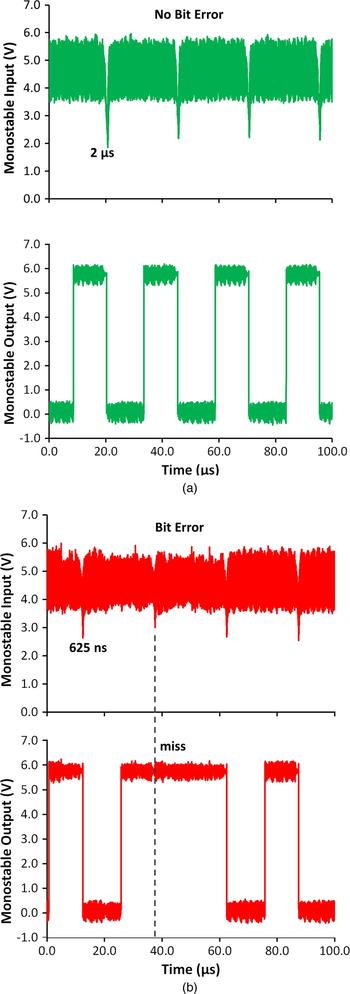
To quantify the performance of the communication signal, we generated a continuous 40 kHz bit train and measured the signal-to-noise ratio (S/N) of the received digital signal as the bit pulse width (compression) was reduced until the lowest possible limit was reached where the output of the monostable “missed” a bit, failing to trigger. Figure 5 is a side-by-side comparison of a bit rate without error (Fig. 5(a)) versus one where the monostable failed to trigger (creating an error, Fig. 5(b)). The top signal of Fig. 5 is the input to the monostable from the filter (comparing a “no bit error” 2 µs pulse (left) to a “bit error” 625 ns pulse (right)); the bottom plot is the monostable output with a reconstituted 12.5 µs bitrate. It can be seen that for the 625 ns pulse a “miss” was observed. This miss was detected on average once every 3 s. Continuing to decrease the pulse width resulted in more frequent misses. It should be noted that we used no form of bit error correction. The system was therefore operated in a regime where no bit errors occurred such that the functionality of the robots was stable.

Fig. 5.

(a) Measurement of the input signal received by a robot's monostable multivibrator IC chip along with the stable monostable output to the IR LED. (b) Same measurement as in (a), but for a bit pulse width below the minimum S/N ratio that produces a “miss” in the monostable output.

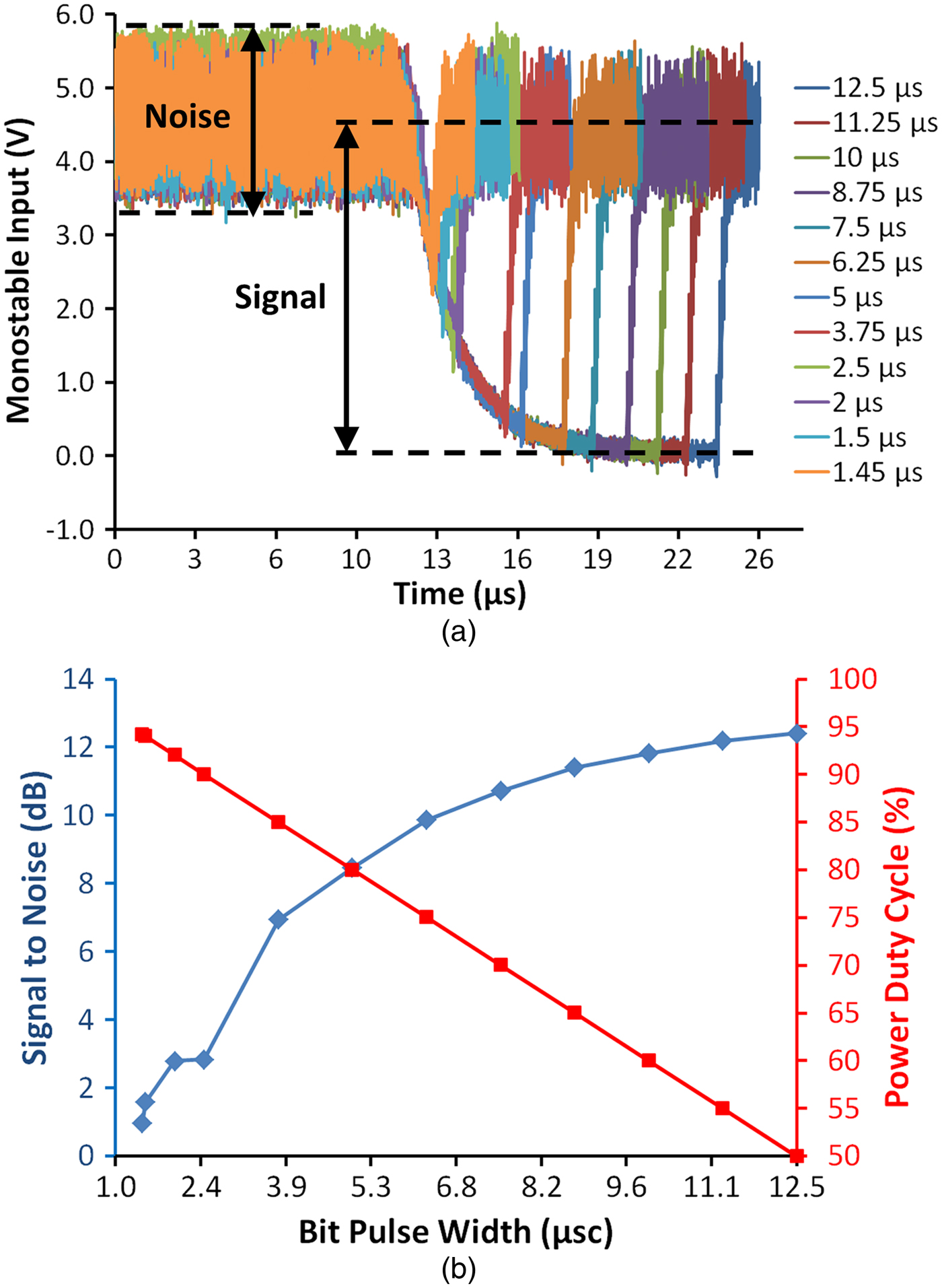
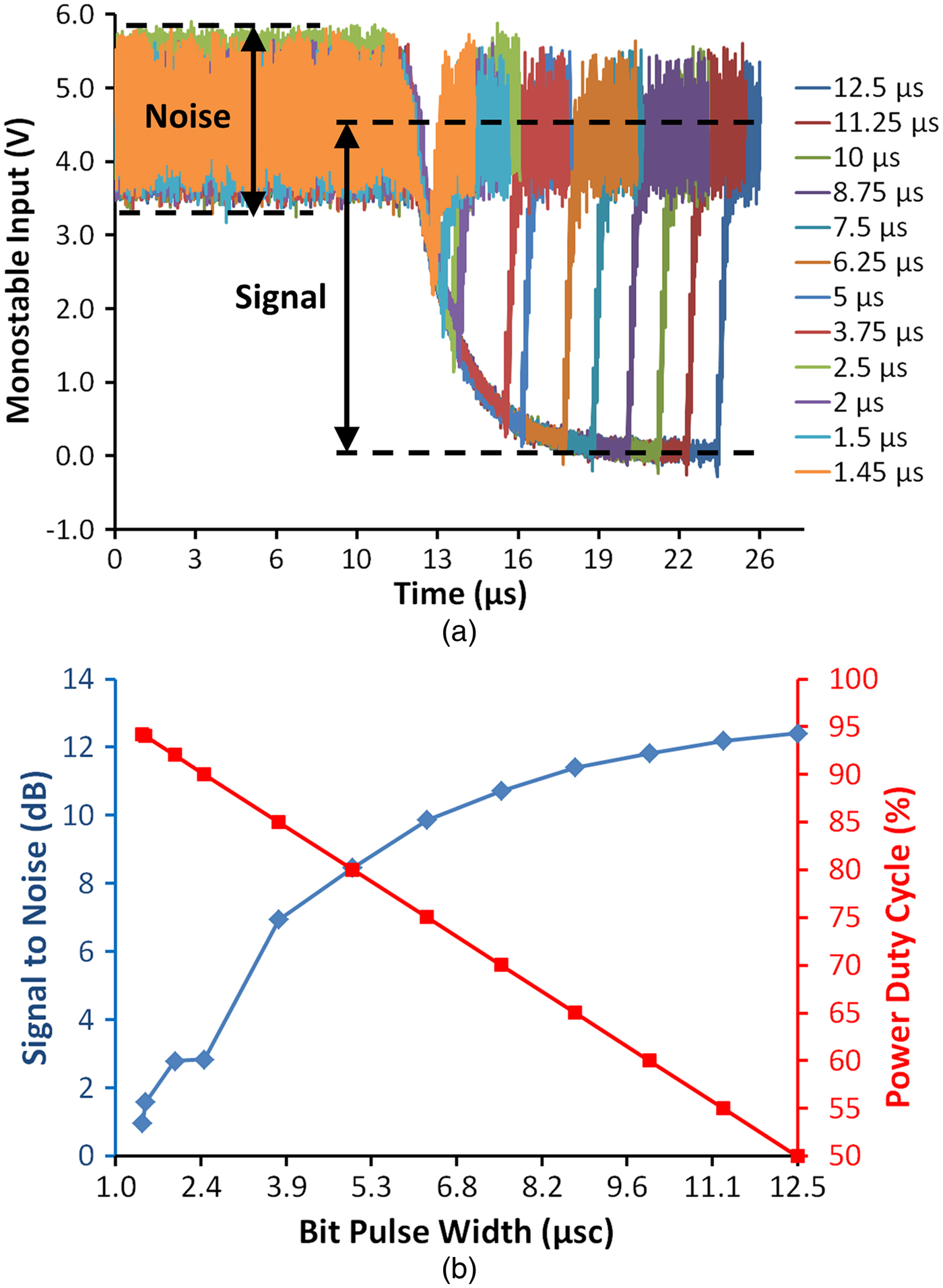
Figure 6(a) shows the signal input to the monostable from the rectified RC filter for varying bit pulse widths. Figure 6(b) is a graph of the S/N depicting the lowest possible S/N to attain stability (i.e. no misses; blue diamond plot) in conjunction with the duty cycle of the applied power (red square plot). The S/N was calculated from the variance of the signal over two bit pulse periods divided by the variance of the noise in the signal (labeled for clarity in Fig. 6(a)). Please note that these plots are for a continuous 40 kHz bit train. The tradeoff for higher S/N is a reduction in the applied power (defined as a power duty cycle, PDC). Bit pulse widths beyond 50% PDC do not significantly improve S/N yet lower the available power to the load. It is therefore advantageous to operate at or near the lowest stable S/N pulse width – especially when multiple mobile devices are active. The theoretical lowest limit of the RC time constant is derived from either the relaxation time of the receiver or the minimum pulse width requirement (MPWR) of the monostable, the slower of these two parameters setting the absolute RC limit. In these experiments the resonator's relaxation was the slower of the two (365 ns as oppose to the monostable's 21 ns MPWR). However, an RC time constant of 1 µs (three times longer than 365 ns) was experimentally observed to work the best due to the half-wave ripple noise in the system (labeled “noise” in Fig. 6(a)). It is possible that with a higher-order filter, the time constant could be made closer to the resonator's relaxation; yielding slightly better S/N than what was obtained.

Fig. 6.

(a) Plot of the monostable input signals from the RC filter on a robot's receiving circuitry with varying bit pulse width. While only one period is shown, the variance of two periods of the “signal” divided by the variance in the “noise” was used to calculate the S/N for different bit pulse widths. (b) A plot of the calculated S/N for each subsequent bit pulse width (blue diamond trace) in combination with the power duty cycle (red square trace) defined as the power signal's on to off ratio percentage.

Using the experimental values, we estimated the number of robots (channel capacity) that could function on the surface with this communication scheme. With a 20 ms command sequence repeating at 77.6 ms intervals, the number of commands that could be placed inside the interval space between command lines was 3 (which would correspond to the maximum number of robots). This assumes that each command line is a separate channel such that each robot only responds to the digital sequence of a particular channel. A 5.87 ms delay between each consecutive command was also added to separate the end of one channel from the beginning of the next. The average PDC for three robots would be 79% without compression and 98% with compression (using a 1.4 µs bit pulse width). It should be noted that the values discussed here are strictly for the Hexbug devices and are centerd on their factory default construction. These are by no means generalized limits. Engineering of both robot and control systems should yield more optimized values. For example, redesigning the robots to function at a higher bit rate would allow a greater number over the surface as the time between successive command lines could be longer.

VI. POWER CONTINUITY AND SCALING

Next we wanted to quantify the level of power continuity over an area by measuring the efficiency at multiple locations across a surface. This is important as the continuity of power is synonymous with the continuity of communication – as our communication scheme is a modulation of the power signal. We used only a single Hexbug for this experiment. The power consumption of the Hexbug was determined by recording the power-draw when connected to a DC power supply. The maximum draw (0.37 W per robot) occurred when the device was moving forward or backward while turning.

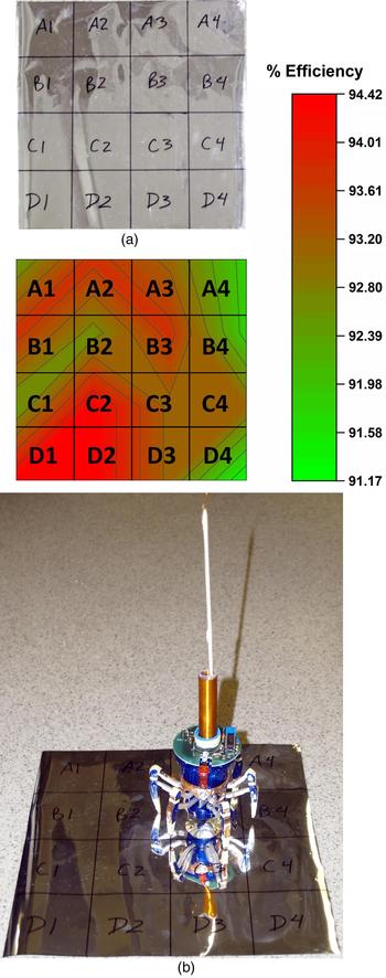
We initially tested the robot's operation on a 28 × 28 cm² metalized polyester sheet. From the perspective of the power supply, the sheet forms a capacitor with the supply neutral. The sheet was divided into grids; with each grid section labeled (Fig. 7). We then powered the robot over each section of the grid, moving the robot in circular (forward while turning) motions, with a fixed driving voltage of 35 VRMS to determine the efficiency profile at each section. We define efficiency as the ratio of the robot's-consumed power (P _LOAD ) versus the real power delivered to the sheet.

(5) $$\eta = \displaystyle{{{P_{LOAD}}} \over {{V_{IN}}{I_{IN}}\cos ({\theta _{XN}})}},$$

where V _IN and I _IN are the input voltage and current, respectively, with their corresponding phase angle θ _XN at X (numeric) and N (alphabetic) grid locations on the sheet, in accordance with Fig. 7(a) (top).

Fig. 7.

(a) Photograph of a 28 × 28 cm² sheet metalized polyester sheet with grids. (b) Contour plot of the average measured efficiency over each grid section of the sheet. (bottom) A photograph of the robot on the sheet showing its scale in proportion to the sheet.

Without the robot present, the input power was purely reactive with a measured phase of −90°. Placement of the robot onto the surface made no observable change. Only when the robot was operating did the input phase angle alter, going from −90° (a purely capacitive load) to −83°. Figure 7(b) (top) shows the measured efficiency at each grid section graphed as a contour plot. From the figure, only a 3% change in efficiency was measured, the difference being due to measurement error as the robot's forward turning movement over each grid was not precise. The averaged efficiency of all sections combined was approximately 93%.

The sheet area was increased to determine the effect of scaling. Changes of the input phase angle became harder to measure as the sheet size expanded. On a 1 × 1 m² sheet, the effect of the robot on the phase angle was not detectable. This was due to the active power consumption of the robot being small compared with the reactive power supplied to the sheet (0.376 W active power to 22.6 VAR reactive power). Such a large ratio made the angle change too small for us to measure.

The largest effect found by expanding the sheet size was the need to increase the drive voltage to operate the robots at full power. The drive voltage can be related to the surface energy placed on the sheet by

(6) $$\Psi = \displaystyle{E \over A} = \displaystyle{{C{V^2}} \over {2A}},$$

where Ψ is the energy per unit area (J/m²), C is the capacitance, V the voltage, and A the surface area. If the area is increased and the applied voltage remains fixed, then the total surface energy reduces. Keeping the surface energies the same, a scaling factor (α) may be derived to determine the required voltage needed for a surface of a larger size

(7) $$\alpha = {\left[ {\displaystyle{{{C_0}} \over {{A_0}}}\displaystyle{{{A_1}} \over {{C_1}}}} \right]^{1/2}},$$

where C ₀ is the initial capacitance, A ₀ is the initial surface area, C ₁ is the scaled capacitance, and A ₁ is the scaled surface area. Multiplying α by the initial voltage yields the voltage needed for a larger area. Likewise, the inverse of α can be used to determine the voltage for a smaller area.

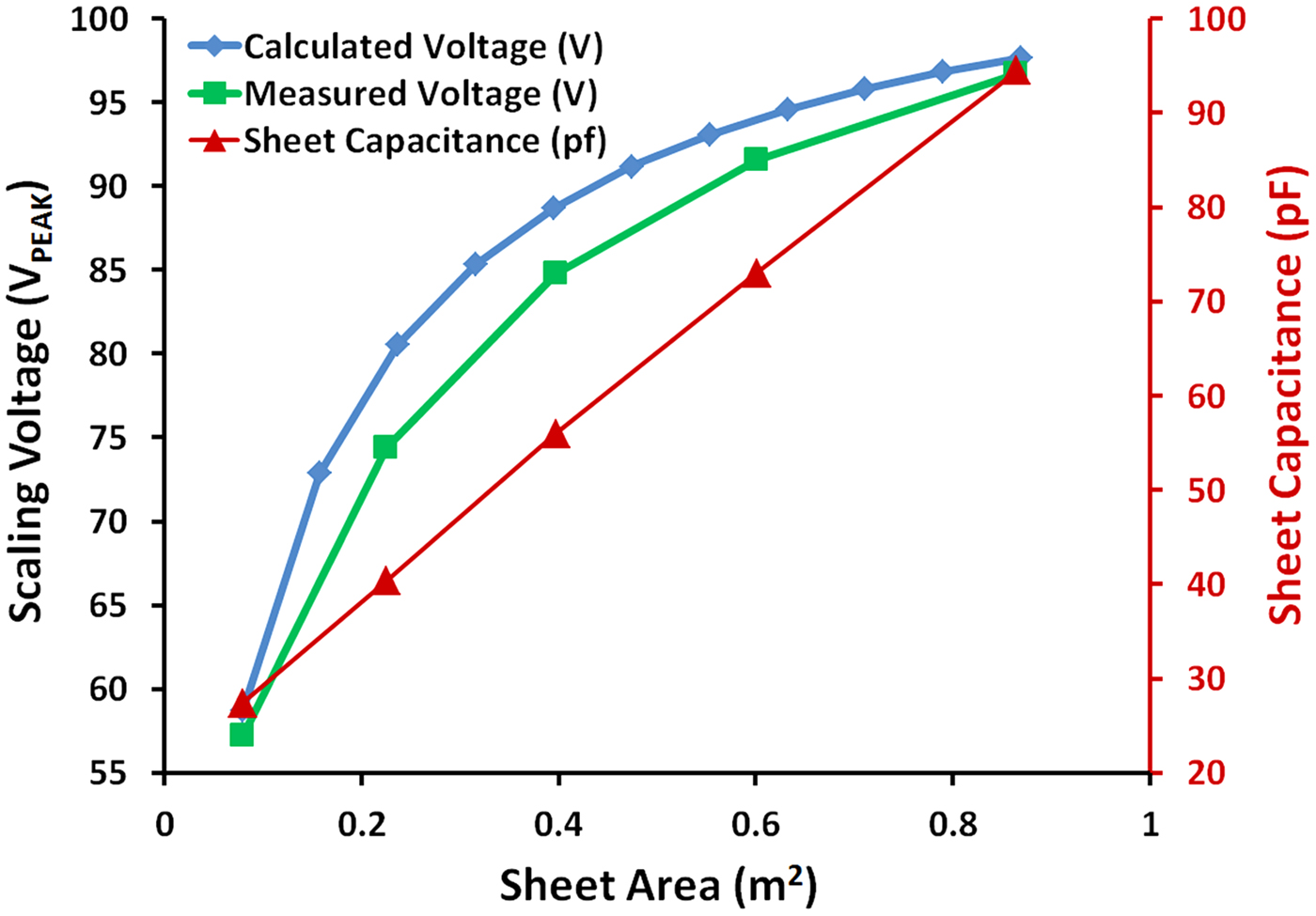
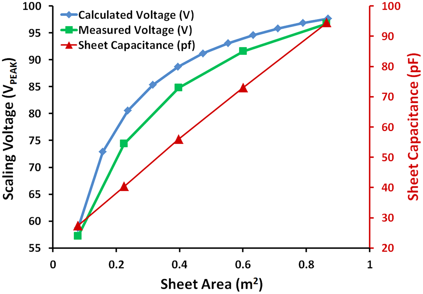
To verify equation (7), the capacitance of five different sheet sizes were measured: 28 × 28 cm² (0.079 m²), 47 × 47 cm² (0.225 m²), 63 × 63 cm² (0.397 m²), 77 × 77 cm² (0.600 m²), and 93 × 93 cm² (0.865 m²). Figure 8 is a plot of the measured values for each sheet. It can be seen that the capacitance increase was approximately linear. A single robot was placed on each sheet and the voltage was increased until full power was delivered. The full power voltage was recorded for each sheet size. The measured values were then compared with calculated values. These calculations were based on the 28 × 28 cm² sheet capacitance (27.3 pF) as the starting value. The slope of the measured capacitance in Fig. 8 (red triangle) was used to determine the incremented capacitance per area in the calculation. The measured versus calculated are in close approximation.

Fig. 8.

Left: Calculated versus measured voltages required to produce maximum power to the robotic devices using the scaling factor (α). Right: Plot of the measured capacitance of five different sheet sizes of increasing area: 28 × 28 cm² (0.079 m²), 47 × 47 cm² (0.225 m²), 63 × 63 cm² (0.397 m²), 77 × 77 cm² (0.600 m²), and 93 × 93 cm² (0.865 m²).

Operating two robots over the largest insulated surface tested (~1 × 1 m²) displayed no loss of power continuity or control when the appropriate voltage level was used (~100 V peak). However, it was observed that if the two devices came within 24 cm distance (as measured from their receiver locations), their resonant frequencies would greatly shift and power/control would be reduced unless retuned. This response approximately matches the theorized extent of the stray capacitance flux; as shown in Fig. 1(b) which depicts the influence of external objects on the resonance of the receiver. This may cause issues for a sheet of multiple devices as robots allowed to approach within the detuning range could not be retuned without affecting the others. Methods around this may include limiting their interaction range mechanically (i.e. putting a stopper/bumper around the devices) or by auto-tuning of the receiver by increasing/decreasing the number of windings through electronic means (analog multiplexer, etc.)