2 Preliminaries

We introduce a set of (right-handed) spherical coordinates $(r^{\prime },\unicode[STIX]{x1D703},\unicode[STIX]{x1D719})$ : $r^{\prime }$ is the distance from the centre of the sphere, $\unicode[STIX]{x1D703}$ (with $0\leqslant \unicode[STIX]{x1D703}\leqslant \unicode[STIX]{x03C0}$ ) is the polar angle (and then $\unicode[STIX]{x03C0}/2-\unicode[STIX]{x1D703}$ is the angle of latitude); $\unicode[STIX]{x1D719}$ (with $0\leqslant \unicode[STIX]{x1D719}<2\unicode[STIX]{x03C0}$ ) is the azimuthal angle i.e. the angle of longitude. We use primes, throughout the formulation of the problem, to denote physical (dimensional) variables; these will be removed when we non-dimensionalize. The unit vectors in this $(r^{\prime },\unicode[STIX]{x1D703},\unicode[STIX]{x1D719})$ -system are $(\hat{\boldsymbol{e}}_{r},\hat{\boldsymbol{e}}_{\unicode[STIX]{x1D703}},\hat{\boldsymbol{e}}_{\unicode[STIX]{x1D719}})$ , respectively, and the corresponding velocity components are $(w^{\prime },v^{\prime },u^{\prime })$ ; $\hat{\boldsymbol{e}}_{\unicode[STIX]{x1D719}}$ points from west to east, and $\hat{\boldsymbol{e}}_{\unicode[STIX]{x1D703}}$ 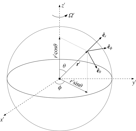from north to south (see figure 1). The governing equations for inviscid flow are the Euler equation

(2.1) $$\begin{eqnarray}\displaystyle & & \displaystyle \left(\frac{\unicode[STIX]{x2202}}{\unicode[STIX]{x2202}t^{\prime }}+\frac{u^{\prime }}{r^{\prime }\sin \unicode[STIX]{x1D703}}\frac{\unicode[STIX]{x2202}}{\unicode[STIX]{x2202}\unicode[STIX]{x1D719}}+\frac{v^{\prime }}{r^{\prime }}\frac{\unicode[STIX]{x2202}}{\unicode[STIX]{x2202}\unicode[STIX]{x1D703}}+w^{\prime }\frac{\unicode[STIX]{x2202}}{\unicode[STIX]{x2202}r^{\prime }}\right)(w^{\prime },v^{\prime },u^{\prime })\nonumber\\ \displaystyle & & \displaystyle \qquad +\,\frac{1}{r^{\prime }}(-u^{\prime 2}-v^{\prime 2},-u^{\prime 2}\cot \unicode[STIX]{x1D703}+v^{\prime }w^{\prime },u^{\prime }v^{\prime }\cot \unicode[STIX]{x1D703}+u^{\prime }w^{\prime })\nonumber\\ \displaystyle & & \displaystyle \qquad +\,2\unicode[STIX]{x1D6FA}^{\prime }(-u^{\prime }\sin \unicode[STIX]{x1D703},-u^{\prime }\cos \unicode[STIX]{x1D703},v^{\prime }\cos \unicode[STIX]{x1D703}+w^{\prime }\sin \unicode[STIX]{x1D703})-r^{\prime }\unicode[STIX]{x1D6FA}^{\prime 2}(\sin ^{2}\unicode[STIX]{x1D703},\sin \unicode[STIX]{x1D703}\cos \unicode[STIX]{x1D703},0)\nonumber\\ \displaystyle & & \displaystyle \quad =-\,\frac{1}{\unicode[STIX]{x1D70C}^{\prime }}\left(\frac{\unicode[STIX]{x2202}p^{\prime }}{\unicode[STIX]{x2202}r^{\prime }},\frac{1}{r^{\prime }}\frac{\unicode[STIX]{x2202}p^{\prime }}{\unicode[STIX]{x2202}\unicode[STIX]{x1D703}},\frac{1}{r^{\prime }\sin \unicode[STIX]{x1D703}}\frac{\unicode[STIX]{x2202}p^{\prime }}{\unicode[STIX]{x2202}\unicode[STIX]{x1D719}}\right)+(-g^{\prime },0,0),\end{eqnarray}$$

and the equation of mass conservation

(2.2) $$\begin{eqnarray}\frac{1}{r^{\prime }\sin \unicode[STIX]{x1D703}}\frac{\unicode[STIX]{x2202}u^{\prime }}{\unicode[STIX]{x2202}\unicode[STIX]{x1D719}}+\frac{1}{r^{\prime }\sin \unicode[STIX]{x1D703}}\frac{\unicode[STIX]{x2202}}{\unicode[STIX]{x2202}\unicode[STIX]{x1D703}}(v^{\prime }\sin \unicode[STIX]{x1D703})+\frac{1}{r^{\prime 2}}\frac{\unicode[STIX]{x2202}}{\unicode[STIX]{x2202}r^{\prime }}(r^{\prime 2}w^{\prime })=0,\end{eqnarray}$$

respectively, where $p^{\prime }(r^{\prime },\unicode[STIX]{x1D703},\unicode[STIX]{x1D719},t^{\prime })$ is the pressure in the fluid, $\unicode[STIX]{x1D6FA}^{\prime }\approx 7.29\times 10^{-5}~\text{rad}~\text{s}^{-1}$ is the constant rate of rotation of the Earth and $\unicode[STIX]{x1D70C}^{\prime }$ is the constant density, with the choice $g^{\prime }=\text{const.}\approx 9.81~\text{m}~\text{s}^{-2}$ for the gravitational term reasonable for the depths of the oceans on the Earth (see Vallis Reference Vallis2006).

Figure 1.

The Earth’s rotating spherical coordinate system: $\unicode[STIX]{x1D703}$ is the polar angle, $\unicode[STIX]{x1D719}$ is the angle of longitude and $r^{\prime }=|\boldsymbol{r}^{\prime }|$ is the distance from the origin at the Earth’s centre. The North Pole is at $\unicode[STIX]{x1D703}=0$ and the Equator is on $\unicode[STIX]{x1D703}=\unicode[STIX]{x03C0}/2$ .

Redefining the pressure

(2.3) $$\begin{eqnarray}p^{\prime }=g^{\prime }\unicode[STIX]{x1D70C}^{\prime }(R^{\prime }-r^{\prime })+{\textstyle \frac{1}{2}}\unicode[STIX]{x1D70C}^{\prime }r^{\prime 2}\unicode[STIX]{x1D6FA}^{\prime 2}\sin ^{2}\unicode[STIX]{x1D703}+P^{\prime }(r^{\prime },\unicode[STIX]{x1D703},\unicode[STIX]{x1D719},t^{\prime }),\end{eqnarray}$$

where $R^{\prime }\approx 6378$  km is the Earth’s radius, and then writing

(2.4) $$\begin{eqnarray}r^{\prime }=R^{\prime }+z^{\prime },\end{eqnarray}$$

we non-dimensionalize the governing equations (2.1)–(2.2) for steady flow according to

(2.5a-c ) $$\begin{eqnarray}z^{\prime }=H^{\prime }z,\quad (w^{\prime },v^{\prime },u^{\prime })=U^{\prime }(kw,v,u),\quad P^{\prime }=\unicode[STIX]{x1D70C}^{\prime }U^{\prime 2}P,\end{eqnarray}$$

where $H^{\prime }$ is the mean depth of the ocean and $U^{\prime }$ is a suitable horizontal speed scale (typically of the order of 4 km and $0.1~\text{m}~\text{s}^{-1}$ , respectively). The scaling factor, $k$ , associated with the vertical component ( $w$ ) of the velocity, is very small (of the order of $10^{-4}$ ) since the vertical motion is so weak that it is almost always inferred rather than measured directly (see Viudez & Dritschel Reference Viudez and Dritschel2015; Marshall & Plumb Reference Marshall and Plumb2016). Defining the shallowness parameter $\unicode[STIX]{x1D700}$ by

(2.6) $$\begin{eqnarray}\unicode[STIX]{x1D700}=\frac{H^{\prime }}{R^{\prime }},\end{eqnarray}$$

the steady-state Euler equations become

(2.7) $$\begin{eqnarray}\displaystyle & & \displaystyle \left(\frac{u}{(1+\unicode[STIX]{x1D700}z)\sin \unicode[STIX]{x1D703}}\frac{\unicode[STIX]{x2202}}{\unicode[STIX]{x2202}\unicode[STIX]{x1D719}}+\frac{v}{1+\unicode[STIX]{x1D700}z}\frac{\unicode[STIX]{x2202}}{\unicode[STIX]{x2202}\unicode[STIX]{x1D703}}+\frac{k}{\unicode[STIX]{x1D700}}w\frac{\unicode[STIX]{x2202}}{\unicode[STIX]{x2202}z}\right)(kw,v,u)\nonumber\\ \displaystyle & & \displaystyle \qquad +\,\frac{1}{1+\unicode[STIX]{x1D700}z}(-u^{2}-v^{2},-u^{2}\cot \unicode[STIX]{x1D703}+kvw,uv\cot \unicode[STIX]{x1D703}+kuw)\nonumber\\ \displaystyle & & \displaystyle \qquad +\,2\unicode[STIX]{x1D714}(-u\sin \unicode[STIX]{x1D703},-u\cos \unicode[STIX]{x1D703},v\cos \unicode[STIX]{x1D703}+kw\sin \unicode[STIX]{x1D703})\nonumber\\ \displaystyle & & \displaystyle \quad =-\left(\frac{1}{\unicode[STIX]{x1D700}}\frac{\unicode[STIX]{x2202}P}{\unicode[STIX]{x2202}z},\frac{1}{1+\unicode[STIX]{x1D700}z}\frac{\unicode[STIX]{x2202}P}{\unicode[STIX]{x2202}\unicode[STIX]{x1D703}},\frac{1}{(1+\unicode[STIX]{x1D700}z)\sin \unicode[STIX]{x1D703}}\frac{\unicode[STIX]{x2202}P}{\unicode[STIX]{x2202}\unicode[STIX]{x1D719}}\right),\end{eqnarray}$$

where

(2.8) $$\begin{eqnarray}\unicode[STIX]{x1D714}=\frac{\unicode[STIX]{x1D6FA}^{\prime }R^{\prime }}{U^{\prime }}\gg 1,\end{eqnarray}$$

(with $\unicode[STIX]{x1D714}\approx 4650$ for $U^{\prime }=0.1~\text{m}~\text{s}^{-1}$ ), while the equation of mass conservation becomes

(2.9) $$\begin{eqnarray}\frac{1}{(1+\unicode[STIX]{x1D700}z)\sin \unicode[STIX]{x1D703}}\left\{\frac{\unicode[STIX]{x2202}u}{\unicode[STIX]{x2202}\unicode[STIX]{x1D719}}+\frac{\unicode[STIX]{x2202}}{\unicode[STIX]{x2202}\unicode[STIX]{x1D703}}(v\sin \unicode[STIX]{x1D703})\right\}+\frac{k}{\unicode[STIX]{x1D700}(1+\unicode[STIX]{x1D700}z)^{2}}\frac{\unicode[STIX]{x2202}}{\unicode[STIX]{x2202}z}\{(1+\unicode[STIX]{x1D700}z)^{2}w\}=0.\end{eqnarray}$$

Typically $k=O(\unicode[STIX]{x1D700}^{2})$ (see the discussion in Constantin & Johnson Reference Constantin and Johnson2017) so that, multiplying the first component of (2.7) by $\unicode[STIX]{x1D700}$ and subsequently letting $\unicode[STIX]{x1D700}\rightarrow 0$ (the shallow-water approximation), we see that the horizontal flow $(u,v)$ is governed by the equations

(2.10) $$\begin{eqnarray}\displaystyle & \displaystyle 0=\frac{\unicode[STIX]{x2202}P}{\unicode[STIX]{x2202}z}, & \displaystyle\end{eqnarray}$$

(2.11) $$\begin{eqnarray}\displaystyle & \displaystyle \left(\frac{u}{\sin \unicode[STIX]{x1D703}}\frac{\unicode[STIX]{x2202}}{\unicode[STIX]{x2202}\unicode[STIX]{x1D719}}+v\frac{\unicode[STIX]{x2202}}{\unicode[STIX]{x2202}\unicode[STIX]{x1D703}}\right)v-u^{2}\cot \unicode[STIX]{x1D703}-2\unicode[STIX]{x1D714}u\cos \unicode[STIX]{x1D703}=-\frac{\unicode[STIX]{x2202}P}{\unicode[STIX]{x2202}\unicode[STIX]{x1D703}}, & \displaystyle\end{eqnarray}$$

(2.12) $$\begin{eqnarray}\displaystyle & \displaystyle \left(\frac{u}{\sin \unicode[STIX]{x1D703}}\frac{\unicode[STIX]{x2202}}{\unicode[STIX]{x2202}\unicode[STIX]{x1D719}}+v\frac{\unicode[STIX]{x2202}}{\unicode[STIX]{x2202}\unicode[STIX]{x1D703}}\right)u+uv\cot \unicode[STIX]{x1D703}+2\unicode[STIX]{x1D714}v\cos \unicode[STIX]{x1D703}=-\frac{1}{\sin \unicode[STIX]{x1D703}}\frac{\unicode[STIX]{x2202}P}{\unicode[STIX]{x2202}\unicode[STIX]{x1D719}}, & \displaystyle\end{eqnarray}$$

(2.13) $$\begin{eqnarray}\displaystyle & \displaystyle \frac{\unicode[STIX]{x2202}u}{\unicode[STIX]{x2202}\unicode[STIX]{x1D719}}+\frac{\unicode[STIX]{x2202}}{\unicode[STIX]{x2202}\unicode[STIX]{x1D703}}(v\sin \unicode[STIX]{x1D703})=0. & \displaystyle\end{eqnarray}$$

The existence of a streamfunction, $\unicode[STIX]{x1D713}(\unicode[STIX]{x1D703},\unicode[STIX]{x1D719})$ , satisfying

(2.14a,b ) $$\begin{eqnarray}u=-\frac{\unicode[STIX]{x2202}\unicode[STIX]{x1D713}}{\unicode[STIX]{x2202}\unicode[STIX]{x1D703}},\quad v=\frac{1}{\sin \unicode[STIX]{x1D703}}\frac{\unicode[STIX]{x2202}\unicode[STIX]{x1D713}}{\unicode[STIX]{x2202}\unicode[STIX]{x1D719}},\end{eqnarray}$$

is ensured by (2.13) and the elimination of the pressure between (2.11) and (2.12) gives the vorticity equation

(2.15) $$\begin{eqnarray}\left(\unicode[STIX]{x1D713}_{\unicode[STIX]{x1D719}}\frac{\unicode[STIX]{x2202}}{\unicode[STIX]{x2202}\unicode[STIX]{x1D703}}-\unicode[STIX]{x1D713}_{\unicode[STIX]{x1D703}}\frac{\unicode[STIX]{x2202}}{\unicode[STIX]{x2202}\unicode[STIX]{x1D719}}\right)\left(\frac{1}{\sin ^{2}\unicode[STIX]{x1D703}}\unicode[STIX]{x1D713}_{\unicode[STIX]{x1D719}\unicode[STIX]{x1D719}}+\unicode[STIX]{x1D713}_{\unicode[STIX]{x1D703}}\cot \unicode[STIX]{x1D703}+\unicode[STIX]{x1D713}_{\unicode[STIX]{x1D703}\unicode[STIX]{x1D703}}-2\unicode[STIX]{x1D714}\cos \unicode[STIX]{x1D703}\right)=0,\end{eqnarray}$$

in which subscripts are used for partial derivatives and

(2.16) $$\begin{eqnarray}\unicode[STIX]{x1D6FB}_{\unicode[STIX]{x1D6F4}}^{2}\unicode[STIX]{x1D713}=\frac{1}{\sin ^{2}\unicode[STIX]{x1D703}}\unicode[STIX]{x1D713}_{\unicode[STIX]{x1D719}\unicode[STIX]{x1D719}}+\unicode[STIX]{x1D713}_{\unicode[STIX]{x1D703}}\cot \unicode[STIX]{x1D703}+\unicode[STIX]{x1D713}_{\unicode[STIX]{x1D703}\unicode[STIX]{x1D703}}\end{eqnarray}$$

is the Laplace–Beltrami expression. Writing (2.15) in the form

(2.17) $$\begin{eqnarray}\unicode[STIX]{x1D713}_{\unicode[STIX]{x1D719}}(\unicode[STIX]{x1D6FB}_{\unicode[STIX]{x1D6F4}}^{2}\unicode[STIX]{x1D713}-2\unicode[STIX]{x1D714}\cos \unicode[STIX]{x1D703})_{\unicode[STIX]{x1D703}}-\unicode[STIX]{x1D713}_{\unicode[STIX]{x1D703}}(\unicode[STIX]{x1D6FB}_{\unicode[STIX]{x1D6F4}}^{2}\unicode[STIX]{x1D713}-2\unicode[STIX]{x1D714}\cos \unicode[STIX]{x1D703})_{\unicode[STIX]{x1D719}}=0,\end{eqnarray}$$

throughout regions where $\unicode[STIX]{x1D735}_{(\unicode[STIX]{x1D719},\unicode[STIX]{x1D703})}\unicode[STIX]{x1D713}\neq (0,0)$ , the rank theorem (see Newns Reference Newns1967) yields

(2.18) $$\begin{eqnarray}\unicode[STIX]{x1D6FB}_{\unicode[STIX]{x1D6F4}}^{2}\unicode[STIX]{x1D713}-2\unicode[STIX]{x1D714}\cos \unicode[STIX]{x1D703}=F(\unicode[STIX]{x1D713})\end{eqnarray}$$

for some function $F$ . The total vorticity of the flow comprises two components: the vorticity solely due to the rotation of the Earth ( $2\unicode[STIX]{x1D714}\cos \unicode[STIX]{x1D703}$ : ‘spin vorticity’) and that due to the underlying motion of the ocean, $F(\unicode[STIX]{x1D713})$ , and not driven by the rotation of the Earth (‘oceanic’ or ‘relative’ vorticity). One of these contributions (the spin vorticity) is completely prescribed, but that associated with the movement of the ocean is specific to the particular flow conditions. Note that if we ignore the planetary (spin) vorticity by setting $\unicode[STIX]{x1D714}=0$ , equation (2.18) becomes the equation describing stationary vortex structures in an ideal fluid. The presence of planetary vorticity in (2.18) alters considerably the underlying mathematical structure of the problem due to the intricate coupling between the oceanic and the planetary vorticity components. For theoretical investigations of vortex dynamics in a bounded region of the surface of a non-rotating sphere we refer to Kidambi & Newton (Reference Kidambi and Newton2000), Newton (Reference Newton2001), Crowdy (Reference Crowdy2006).

Figure 2.

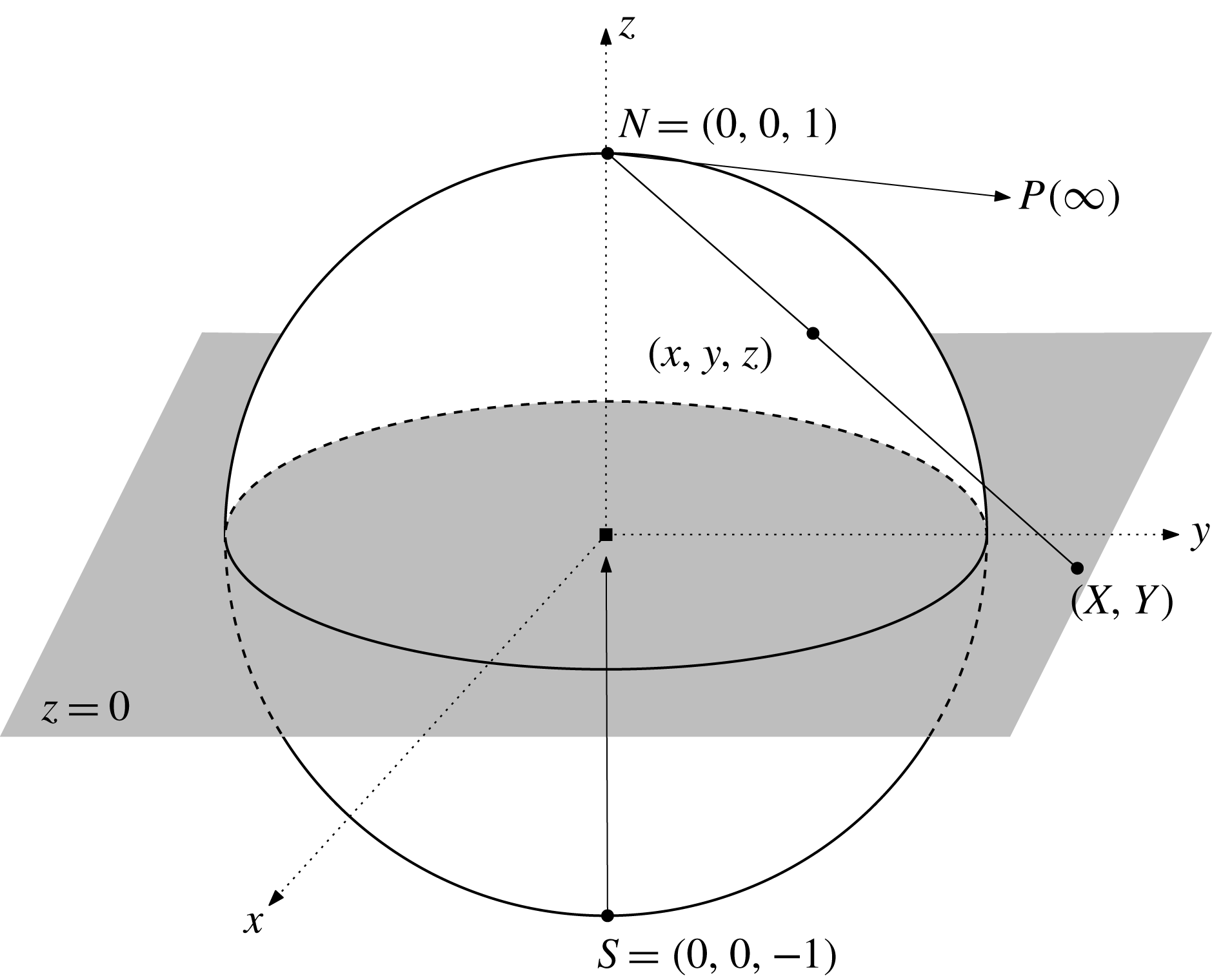
Schematic illustration of the stereographic projection mapping the point $(x,y,z)$ on the unit sphere with the North Pole $N$ excised to the intersection point $(X,Y)$ of the equatorial plane with the ray from $N$ to $(x,y,z)$ .

Equation (2.18) is the counterpart in spherical coordinates of Fofonoff’s $\unicode[STIX]{x1D6FD}$ -plane model Fofonoff (Reference Fofonoff1954), described in modern notation in Vallis (Reference Vallis2006), and offers some exciting prospects for future investigations. For example, on the stereographically projected equatorial $\unicode[STIX]{x1D709}$ -plane, equation (2.18) becomes

(2.19) $$\begin{eqnarray}(1+\unicode[STIX]{x1D709}\overline{\unicode[STIX]{x1D709}})^{2}\unicode[STIX]{x1D713}_{\unicode[STIX]{x1D709}\overline{\unicode[STIX]{x1D709}}}=2\unicode[STIX]{x1D714}\frac{\unicode[STIX]{x1D709}\overline{\unicode[STIX]{x1D709}}-1}{1+\unicode[STIX]{x1D709}\overline{\unicode[STIX]{x1D709}}}+F(\unicode[STIX]{x1D713}),\end{eqnarray}$$

where $|\unicode[STIX]{x1D709}|=\cot (\unicode[STIX]{x1D703}/2)$ for the polar angle $\unicode[STIX]{x1D703}\in (0,\unicode[STIX]{x03C0})$ ; see figure 2. Explicit solutions for linear functions $F$ were obtained in Constantin & Johnson (Reference Constantin and Johnson2017), e.g. for $F=\unicode[STIX]{x1D6FE}$ (const.), the general solution of (2.19) is given by

(2.20) $$\begin{eqnarray}\unicode[STIX]{x1D713}(\unicode[STIX]{x1D709},\overline{\unicode[STIX]{x1D709}})=\unicode[STIX]{x1D6FE}\ln (1+\unicode[STIX]{x1D709}\overline{\unicode[STIX]{x1D709}})+\frac{2\unicode[STIX]{x1D714}}{1+\unicode[STIX]{x1D709}\overline{\unicode[STIX]{x1D709}}}+\unicode[STIX]{x1D707}(\unicode[STIX]{x1D709},\overline{\unicode[STIX]{x1D709}}),\end{eqnarray}$$

where $\unicode[STIX]{x1D707}(\unicode[STIX]{x1D709},\overline{\unicode[STIX]{x1D709}})$ is an arbitrary harmonic function. The considerations related to Stuart vortices (see Stuart Reference Stuart1967; Crowdy Reference Crowdy2004) offer prospects for the study of the nonlinear vorticity function $F(\unicode[STIX]{x1D713})=a\text{e}^{b\unicode[STIX]{x1D713}}+c$ with suitable real constants  $a$ ,  $b$ ,  $c$ .

3 Main result

We seek solutions of (2.19) for $F(\unicode[STIX]{x1D713})=a\text{e}^{b\unicode[STIX]{x1D713}}+c$ with suitable real constants  $a$ , $b$ , $c$ . Setting

(3.1) $$\begin{eqnarray}\unicode[STIX]{x1D713}(\unicode[STIX]{x1D709},\overline{\unicode[STIX]{x1D709}})=\unicode[STIX]{x1D701}(\unicode[STIX]{x1D709},\overline{\unicode[STIX]{x1D709}})+A\ln (1+\unicode[STIX]{x1D709}\overline{\unicode[STIX]{x1D709}}),\end{eqnarray}$$

for some real constant $A$ to be determined, we get

(3.2a,b ) $$\begin{eqnarray}\unicode[STIX]{x1D713}_{\unicode[STIX]{x1D709}\overline{\unicode[STIX]{x1D709}}}=\unicode[STIX]{x1D701}_{\unicode[STIX]{x1D709}\overline{\unicode[STIX]{x1D709}}}+\frac{A}{(1+\unicode[STIX]{x1D709}\overline{\unicode[STIX]{x1D709}})^{2}},\quad \text{e}^{b\unicode[STIX]{x1D713}}=(1+\unicode[STIX]{x1D709}\overline{\unicode[STIX]{x1D709}})^{Ab}\text{e}^{b\unicode[STIX]{x1D701}},\end{eqnarray}$$

and therefore (2.19) becomes

(3.3) $$\begin{eqnarray}\unicode[STIX]{x1D701}_{\unicode[STIX]{x1D709}\overline{\unicode[STIX]{x1D709}}}=\frac{c-A+2\unicode[STIX]{x1D714}}{(1+\unicode[STIX]{x1D709}\overline{\unicode[STIX]{x1D709}})^{2}}-\frac{4\unicode[STIX]{x1D714}}{(1+\unicode[STIX]{x1D709}\overline{\unicode[STIX]{x1D709}})^{3}}+a\text{e}^{b\unicode[STIX]{x1D701}}(1+\unicode[STIX]{x1D709}\overline{\unicode[STIX]{x1D709}})^{Ab-2}.\end{eqnarray}$$

For

(3.4a,b ) $$\begin{eqnarray}A=\frac{2}{b},\quad c=A-2\unicode[STIX]{x1D714},\end{eqnarray}$$

we see that (2.19) is transformed to the equation

(3.5) $$\begin{eqnarray}\unicode[STIX]{x1D701}_{\unicode[STIX]{x1D709}\overline{\unicode[STIX]{x1D709}}}=a\text{e}^{b\unicode[STIX]{x1D701}}-\frac{4\unicode[STIX]{x1D714}}{(1+\unicode[STIX]{x1D709}\overline{\unicode[STIX]{x1D709}})^{3}}.\end{eqnarray}$$

Setting $\unicode[STIX]{x1D714}=0$ in (3.5) leads us to the Liouville equation

(3.6) $$\begin{eqnarray}\unicode[STIX]{x1D701}_{\unicode[STIX]{x1D709}\overline{\unicode[STIX]{x1D709}}}=a\text{e}^{b\unicode[STIX]{x1D701}},\end{eqnarray}$$

which is exactly solvable. This feature enabled Crowdy (Reference Crowdy2004) to associate with any solution $\unicode[STIX]{x1D701}_{0}$ of (3.6) an explicit streamfunction

(3.7) $$\begin{eqnarray}\unicode[STIX]{x1D713}_{0}(\unicode[STIX]{x1D709},\overline{\unicode[STIX]{x1D709}})=\unicode[STIX]{x1D701}_{0}(\unicode[STIX]{x1D709},\overline{\unicode[STIX]{x1D709}})+\frac{2}{b}\ln (1+\unicode[STIX]{x1D709}\overline{\unicode[STIX]{x1D709}})\end{eqnarray}$$

that represents the flow pattern of Stuart-type vortices on a non-rotating sphere. We aim to show that for any gyre flow with nonlinear oceanic vorticity of the form

(3.8) $$\begin{eqnarray}F(\unicode[STIX]{x1D713})=a\text{e}^{b\unicode[STIX]{x1D713}}+\frac{2}{b}-2\unicode[STIX]{x1D714},\end{eqnarray}$$

dependent on the inverse Rossby number $\unicode[STIX]{x1D714}\gg 1$ and on the free real parameters $a,b$ with $ab>0$ , and such that the diameter $d^{\prime }$ of the gyre region satisfies

(3.9) $$\begin{eqnarray}d^{\prime }\sqrt{\frac{\unicode[STIX]{x1D6FA}^{\prime }}{U^{\prime }R^{\prime }}}=O(1),\end{eqnarray}$$

the explicit functions in (3.7) are accurate approximations of the streamfunction $\unicode[STIX]{x1D713}$ of the gyre flow, in the sense that

(3.10) $$\begin{eqnarray}0\leqslant \unicode[STIX]{x1D713}-\unicode[STIX]{x1D713}_{0}\leqslant \frac{1}{4}\frac{\sin ^{6}(\unicode[STIX]{x1D703}_{S}/2)}{\sin ^{2}(\unicode[STIX]{x1D703}_{N}/2)}\frac{(d^{\prime })^{2}\unicode[STIX]{x1D6FA}^{\prime }}{U^{\prime }R^{\prime }},\end{eqnarray}$$

where $\unicode[STIX]{x1D703}_{N}\in (0,\unicode[STIX]{x03C0})$ and $\unicode[STIX]{x1D703}_{S}\in (0,\unicode[STIX]{x03C0})$ are the co-latitudes of the northern, respectively southern, tips of the gyre region; here the diameter of a (not necessarily circular) planar or spherical region is defined as the largest distance between two points in the region. Intuitively, this result means that, although the rotation term in (3.5) is large, its effect on the (highly nonlinear) dynamics can nevertheless be small if the size of the gyre region is relatively small, as quantified in (3.9) and (3.10). Physically realistic scenarios for the occurrence of such flows are provided in § 5.

We rely on the theory of elliptic partial differential equations to prove the approximation property (3.10). Indeed, in terms of the Cartesian coordinates $(X,Y)$ in the complex $\unicode[STIX]{x1D709}$ -plane, we can write (3.5) as the semilinear elliptic equation

(3.11) $$\begin{eqnarray}\unicode[STIX]{x0394}\unicode[STIX]{x1D701}=4a\text{e}^{b\unicode[STIX]{x1D701}}-\frac{16\unicode[STIX]{x1D714}}{(1+X^{2}+Y^{2})^{3}},\end{eqnarray}$$

where $\unicode[STIX]{x0394}=\unicode[STIX]{x2202}_{X}^{2}+\unicode[STIX]{x2202}_{Y}^{2}$ is the Laplace operator, while (3.6) becomes

(3.12) $$\begin{eqnarray}\unicode[STIX]{x0394}\unicode[STIX]{x1D701}=4a\text{e}^{b\unicode[STIX]{x1D701}}.\end{eqnarray}$$

At the ocean surface, a gyre is delimited by a level set of the streamfunction, say $\unicode[STIX]{x1D713}=0$ , which encloses a region $O^{\prime }$ on the surface of the sphere and this spherical region corresponds in the $(X,Y)$ -coordinates to a planar region $O$ , the scaled stereographic projection of $O^{\prime }$ . Consequently we have to solve for

(3.13) $$\begin{eqnarray}\unicode[STIX]{x1D6FE}=\unicode[STIX]{x1D701}-\unicode[STIX]{x1D701}_{0}\end{eqnarray}$$

the equation

(3.14) $$\begin{eqnarray}-\unicode[STIX]{x0394}\unicode[STIX]{x1D6FE}+4a\text{e}^{b\unicode[STIX]{x1D701}_{0}}(\text{e}^{b\unicode[STIX]{x1D6FE}}-1)-\frac{16\unicode[STIX]{x1D714}}{(1+X^{2}+Y^{2})^{3}}=0\end{eqnarray}$$

in a bounded planar domain $O$ , with homogeneous Dirichlet boundary data

(3.15) $$\begin{eqnarray}\unicode[STIX]{x1D6FE}=0\quad \text{on}~\unicode[STIX]{x2202}O,\end{eqnarray}$$

where $\unicode[STIX]{x2202}O$ is the smooth boundary of $O$ . In our analysis we apply the method of sub- and super-solutions, combined with maximum principles and elliptic a priori estimates.

We recall that the classical Calderón–Zygmund theory for the linear Dirichlet problem

(3.16) $$\begin{eqnarray}\left.\begin{array}{@{}ll@{}}\unicode[STIX]{x0394}U_{0}=F_{0} & \text{in}~O,\\ U_{0}=0 & \text{on}~\unicode[STIX]{x2202}O,\end{array}\right\}\end{eqnarray}$$

in the setting of Sobolev spaces, asserts that if $F_{0}\in L^{2}(O)$ , then there exists a unique solution $U_{0}\in H^{2}(O)\cap H_{0}^{1}(O)$ of (3.16) and the following estimate holds:

(3.17) $$\begin{eqnarray}\Vert U_{0}\Vert _{H^{2}(O)}\leqslant C_{0}\Vert F_{0}\Vert _{L^{2}(O)}\end{eqnarray}$$

for some constant $C_{0}>0$ depending only on $O$ ; see Brézis (Reference Brézis2011) and Ponce (Reference Ponce2016). Moreover, if $F_{0}$ is the restriction of a continuous function $F_{0}:\mathbb{R}^{2}\rightarrow \mathbb{R}$ to $O$ , then $U_{0}$ is twice continuously differentiable in $O$ and admits a continuous extension to the closure $\overline{O}=O\cup \unicode[STIX]{x2202}O$ of  $O$ ; see Gilbarg & Trudinger (Reference Gilbarg and Trudinger2001). Note that in terms of the Green’s function of the first kind for  $O$ , $G_{O}(X,Y,X^{\prime },Y^{\prime })$ , we have

(3.18) $$\begin{eqnarray}U_{0}(X,Y)=\iint _{O}G_{O}(X,Y,X^{\prime },Y^{\prime })F_{0}(X^{\prime },Y^{\prime })\,\text{d}X^{\prime }\,\text{d}Y^{\prime },\quad (X,Y)\in O.\end{eqnarray}$$

In particular, for circular domains, Green’s function $G_{O}(X,Y,X^{\prime },Y^{\prime })$ is explicitly determined (see Gilbarg & Trudinger Reference Gilbarg and Trudinger2001). Also, for annular domains an explicit Green’s function is available (see Crowdy & Marshall Reference Crowdy and Marshall2007). While the estimate (3.17) and the representation formula (3.18) are important for the existence of solutions, we will take advantage of the following growth estimate for the solution of (3.16):

(3.19) $$\begin{eqnarray}0\leqslant U_{0}(X,Y)\leqslant {\textstyle \frac{1}{16}}MD^{2},\quad (X,Y)\in O,\end{eqnarray}$$

where $D$ is the diameter of the set $O$ and

(3.20) $$\begin{eqnarray}0\leqslant M=\max _{(X,Y)\in \overline{O}}\{-F_{0}(X,Y)\}\quad \text{for}~F_{0}:\overline{O}\rightarrow (-\infty ,0]~\text{continuous}.\end{eqnarray}$$

To prove (3.19), note that since $F_{0}\leqslant 0$ , the weak maximum principle (see Gilbarg & Trudinger Reference Gilbarg and Trudinger2001) ensures that the minimum of the solution $U_{0}$ in $\overline{O}$ is attained on the boundary $\unicode[STIX]{x2202}O$ , and thus $U_{0}\geqslant 0$ throughout $\overline{O}$ . Furthermore, if $(X_{0},Y_{0})\in \overline{O}$ is a point such that $\overline{O}$ is contained within the closed ball of radius $D/2$ centred at this point, then the function $\tilde{U}$ defined by

(3.21) $$\begin{eqnarray}\tilde{U} (X,Y)=U_{0}(X,Y)+\frac{M[4(X-X_{0})^{2}+4(Y-Y_{0})^{2}-D^{2}]}{16},\quad (X,Y)\in \overline{O},\end{eqnarray}$$

is such that $\unicode[STIX]{x0394}\tilde{U} \geqslant 0$ in $O$ and $\tilde{U} \leqslant 0$ on $\unicode[STIX]{x2202}O$ . The weak maximum principle therefore ensures that the maximum of the solution $\tilde{U}$ in $\overline{O}$ is attained on the boundary $\unicode[STIX]{x2202}O$ , so that $\tilde{U} \leqslant 0$ throughout $\overline{O}$ and this proves the upper estimate in (3.19).

On the other hand, twice continuously differentiable functions $\unicode[STIX]{x1D6FE}_{\ast }$ , $\unicode[STIX]{x1D6FE}^{\ast }:O\rightarrow \mathbb{R}$ with continuous extensions to $\overline{O}$ which vanish on the boundary $\unicode[STIX]{x2202}O$ , are called a sub-solution (super-solution) of (3.14) with the homogeneous Dirichlet boundary condition (3.15) if

(3.22) $$\begin{eqnarray}-\unicode[STIX]{x0394}\unicode[STIX]{x1D6FE}_{\ast }+4a\text{e}^{b\unicode[STIX]{x1D701}_{0}}(\text{e}^{b\unicode[STIX]{x1D6FE}_{\ast }}-1)-\frac{16\unicode[STIX]{x1D714}}{(1+X^{2}+Y^{2})^{3}}\leqslant 0,\quad (X,Y)\in O,\end{eqnarray}$$

respectively if

(3.23) $$\begin{eqnarray}-\unicode[STIX]{x0394}\unicode[STIX]{x1D6FE}^{\ast }+4a\text{e}^{b\unicode[STIX]{x1D701}_{0}}(\text{e}^{b\unicode[STIX]{x1D6FE}\ast }-1)-\frac{16\unicode[STIX]{x1D714}}{(1+X^{2}+Y^{2})^{3}}\geqslant 0,\quad (X,Y)\in O.\end{eqnarray}$$

Since the nonlinearity in (3.14) is smooth, the method of sub- and super-solutions applies: the existence of a sub-solution $\unicode[STIX]{x1D6FE}_{\ast }$ and of a super-solution $\unicode[STIX]{x1D6FE}^{\ast }$ with $\unicode[STIX]{x1D6FE}_{\ast }\leqslant \unicode[STIX]{x1D6FE}^{\ast }$ in $O$ ensures the existence of a solution $\unicode[STIX]{x1D6FE}$ that is twice continuously differentiable in  $O$ , admits a continuous extension to $\overline{O}$ and satisfies $\unicode[STIX]{x1D6FE}_{\ast }\leqslant \unicode[STIX]{x1D6FE}\leqslant \unicode[STIX]{x1D6FE}^{\ast }$ throughout $\overline{O}$ ; see Ponce (Reference Ponce2016).

Let now $\unicode[STIX]{x1D701}_{0}$ be a solution of the Liouville equation (3.12), in a domain $O$ delimited by a zero level set of $\unicode[STIX]{x1D713}_{0}$ defined by (3.7), and let $U_{0}$ be the unique solution of (3.16) with the homogeneous Dirichlet boundary condition $U_{0}=0$ on $\unicode[STIX]{x2202}O$ , for

(3.24) $$\begin{eqnarray}F_{0}(X,Y)=-\frac{16\unicode[STIX]{x1D714}}{(1+X^{2}+Y^{2})^{3}}.\end{eqnarray}$$

We now claim that $\unicode[STIX]{x1D6FE}_{\ast }=0$ is a sub-solution and $\unicode[STIX]{x1D6FE}^{\ast }=U_{0}$ is a super-solution of (3.14), with $\unicode[STIX]{x1D6FE}_{\ast }\leqslant \unicode[STIX]{x1D6FE}^{\ast }$ in  $O$ . Indeed, since $F_{0}<0$ , the strong maximum principle (see Gilbarg & Trudinger Reference Gilbarg and Trudinger2001) yields

(3.25) $$\begin{eqnarray}U_{0}(X,Y)>0,\quad (X,Y)\in O,\end{eqnarray}$$

so that $\unicode[STIX]{x1D701}_{\ast }<\unicode[STIX]{x1D701}^{\ast }$ in $O$ and

(3.26) $$\begin{eqnarray}a\text{e}^{b(\unicode[STIX]{x1D701}_{0}+U_{0})}\geqslant a\text{e}^{b\unicode[STIX]{x1D701}_{0}}\quad \text{in}~O~\text{since}~ab>0,\end{eqnarray}$$

with the inequalities (3.22)–(3.23) now easily checked. The method of sub- and super-solutions therefore ensures the existence of a solution $\unicode[STIX]{x1D6FE}$ to (3.14) with homogeneous Dirichlet boundary data (3.15), such that

(3.27) $$\begin{eqnarray}0\leqslant \unicode[STIX]{x1D6FE}\leqslant U_{0}\quad \text{in}~O.\end{eqnarray}$$

Using (3.1), (3.7) and (3.19), we get

(3.28) $$\begin{eqnarray}0\leqslant \unicode[STIX]{x1D713}-\unicode[STIX]{x1D713}_{0}=\unicode[STIX]{x1D6FE}\leqslant U_{0}\leqslant {\textstyle \frac{1}{16}}MD^{2}\quad \text{throughout}~O^{\prime }.\end{eqnarray}$$

Since

(3.29) $$\begin{eqnarray}1+X^{2}+Y^{2}=1+|\unicode[STIX]{x1D709}|^{2}=\frac{1}{\sin ^{2}\left({\displaystyle \frac{\unicode[STIX]{x1D703}}{2}}\right)},\end{eqnarray}$$

we see that (3.24) in combination with (3.28) yields

(3.30) $$\begin{eqnarray}0\leqslant \unicode[STIX]{x1D713}-\unicode[STIX]{x1D713}_{0}\leqslant \unicode[STIX]{x1D714}D^{2}\sin ^{6}\left(\frac{\unicode[STIX]{x1D703}_{S}}{2}\right)\quad \text{throughout}~O^{\prime },\end{eqnarray}$$

where $\unicode[STIX]{x1D703}_{S}$ is the co-latitude of the southern tip of the gyre region $O^{\prime }$ and $D$ is the diameter of the (scaled) planar stereographic projection $O$ of the spherical region  $O^{\prime }$ . Note that the stereographic projection distorts areas, with the infinitesimal distortion rate from the sphere to the plane equal to $4\sin ^{2}(\unicode[STIX]{x1D703}/2)$ ; in particular, planar projections of spherical areas near the South Pole are diminished while the projections of spherical areas near the North Pole are inflated. Therefore the diameter $d^{\prime }$ of the gyre region $O^{\prime }$ satisfies

(3.31) $$\begin{eqnarray}\frac{d^{\prime }}{R^{\prime }}\geqslant 2D\sin \left(\frac{\unicode[STIX]{x1D703}_{N}}{2}\right),\end{eqnarray}$$

where $\unicode[STIX]{x1D703}_{N}$ is the co-latitude of the northern tip of  $O^{\prime }$ . Using the above inequality in (3.30) validates the estimate (3.10), due to (2.8).

Since $\unicode[STIX]{x1D6FE}=\unicode[STIX]{x1D713}-\unicode[STIX]{x1D713}_{0}=\unicode[STIX]{x1D701}-\unicode[STIX]{x1D701}_{0}$ vanishes on $\unicode[STIX]{x2202}O$ , with $\unicode[STIX]{x1D701}_{0}$ and $\unicode[STIX]{x1D713}_{0}$ both known explicitly within  $O$ , to appreciate the relevance of the estimate (3.10) for revealing the streamline pattern of the flow, let us show that the range of (real) values of $\unicode[STIX]{x1D701}_{0}$ throughout $O$ can be very wide for suitable choices of the free parameters $a$ and  $b$ . To prove this, let us assume without loss of generality that $a>0$ , and so $b>0$ . Firstly, since $\unicode[STIX]{x1D713}_{0}=0$ on $\unicode[STIX]{x2202}O$ , from (3.7) we infer that

(3.32) $$\begin{eqnarray}\unicode[STIX]{x1D701}_{0}=-\frac{2}{b}\ln (1+\unicode[STIX]{x1D709}\overline{\unicode[STIX]{x1D709}})\leqslant 0\quad \text{on}~\unicode[STIX]{x2202}O.\end{eqnarray}$$

We now prove that if $m>0$ is such that

(3.33) $$\begin{eqnarray}\frac{4m\text{e}^{bm}}{a}\leqslant d_{0}^{2}.\end{eqnarray}$$

where $d_{0}$ is the diameter of the largest ball contained within the planar region  $O$ , then

(3.34) $$\begin{eqnarray}\inf _{(X,Y)\in O}\{\unicode[STIX]{x1D701}_{0}(X,Y)\}<-m.\end{eqnarray}$$

To verify the estimate (3.34), let us first note that since $\unicode[STIX]{x1D701}_{0}\leqslant 0$ on $\unicode[STIX]{x2202}O$ and $\unicode[STIX]{x0394}\unicode[STIX]{x1D701}_{0}>0$ in $O$ is ensured by the fact that $\unicode[STIX]{x1D701}_{0}$ solves (3.12), the weak maximum principle yields $\unicode[STIX]{x1D701}_{0}<0$ throughout $O$ . If ${\mathcal{B}}_{0}$ is the largest ball contained within the planar region $O$ that is bounded by the smooth streamline $\unicode[STIX]{x1D713}_{0}=0$ , then the circle $\unicode[STIX]{x2202}{\mathcal{B}}_{0}$ that surrounds ${\mathcal{B}}_{0}$ will be tangent to $\unicode[STIX]{x2202}O$ . Define the function

(3.35) $$\begin{eqnarray}\unicode[STIX]{x1D6FC}_{0}(X,Y)=\unicode[STIX]{x1D701}_{0}(X,Y)-\frac{a\text{e}^{-bm}[4(X-X^{0})^{2}+4(Y-Y^{0})^{2}-d_{0}^{2}]}{4},\quad (X,Y)\in {\mathcal{B}}_{0},\end{eqnarray}$$

where $(X^{0},Y^{0})$ is the centre of the disk ${\mathcal{B}}_{0}$ . Assuming that (3.34) is invalid, we would get $\unicode[STIX]{x1D701}_{0}\geqslant -m$ throughout $O$ , and (3.12) would yield $\unicode[STIX]{x0394}\unicode[STIX]{x1D701}_{0}\geqslant 4a\text{e}^{-bm}$ in ${\mathcal{B}}_{0}\subset O$ . But then, since $\unicode[STIX]{x1D6FC}_{0}\leqslant 0$ on $\unicode[STIX]{x2202}{\mathcal{B}}_{0}$ and $\unicode[STIX]{x0394}\unicode[STIX]{x1D6FC}_{0}=\unicode[STIX]{x0394}\unicode[STIX]{x1D701}_{0}-4a\text{e}^{-bm}\geqslant 0$ in ${\mathcal{B}}_{0}$ , the weak maximum principle would ensure that $\unicode[STIX]{x1D6FC}_{0}<0$ throughout ${\mathcal{B}}_{0}$ . In particular, $\unicode[STIX]{x1D6FC}_{0}(X^{0},Y^{0})<0$ , that is,

(3.36) $$\begin{eqnarray}\unicode[STIX]{x1D701}_{0}(X^{0},Y^{0})<-\frac{a\text{e}^{-bm}}{4}d_{0}^{2}.\end{eqnarray}$$

But (3.33) then leads us to $\unicode[STIX]{x1D701}_{0}(X^{0},Y^{0})<-m$ , which is in contradiction with the assumption of the invalidity of (3.34). Consequently (3.34) must hold.

The estimates (3.10), (3.32) and (3.34) show that if the diameter of the gyre region satisfies (3.9), then the streamline pattern for $\unicode[STIX]{x1D713}$ is a small perturbation of the level sets of the explicit function  $\unicode[STIX]{x1D713}_{0}$ .

4 Flow visualization

The form of the general solution to the Liouville equation (3.6) is (see Crowdy Reference Crowdy1997; Henrici Reference Henrici1986)

(4.1) $$\begin{eqnarray}\unicode[STIX]{x1D701}(z,\bar{z})=\frac{1}{b}\log \left(\frac{4|f^{\prime }(z)|^{2}}{(2-ab|f(z)|^{2})^{2}}\right),\end{eqnarray}$$

where $f$ is a meromorphic function with $f^{\prime }\neq 0$ , $|f|\neq \sqrt{2}/\sqrt{ab}$ , and having at most isolated simple pole singularities in the domain in which the equation is to be solved. By means of (3.1) and (4.1), we can visualize the streamlines for various choices of $f$ (see figure 3 for an example that captures the flow pattern of a large gyre). For a given  $f$ , any closed streamline can be used to define the boundary of the relevant flow region. Note that typical gyre regions on the surface of the sphere are mapped by the stereographic projection into simply connected regions of the complex plane, for which the representation of Green’s function (corresponding to the Laplace operator) by the Riemann mapping function is classical (see Henrici Reference Henrici1986). Moreover, we can approximate the boundary of a region of specific geophysical interest by a polygonal line with a high degree of accuracy, in which case the Schwarz–Christoffel formulas provide an explicit representation for the Riemann mapping function (see Henrici Reference Henrici1986). In this context, we point out that if $O$ is a simply connected bounded region of the complex plane, and $\mathfrak{g}(z,z^{\prime })=-\text{log}|z-z^{\prime }|-\mathfrak{h}(z,z^{\prime })$ is its Green’s function for the Laplace operator, then $\unicode[STIX]{x1D701}(\unicode[STIX]{x1D709})=\mathfrak{h}(\unicode[STIX]{x1D709},\unicode[STIX]{x1D709})$ solves Liouville’s equation $\unicode[STIX]{x0394}\unicode[STIX]{x1D701}=4\text{e}^{2\unicode[STIX]{x1D701}}$ (see Gustafsson Reference Gustafsson1990).

Figure 3.

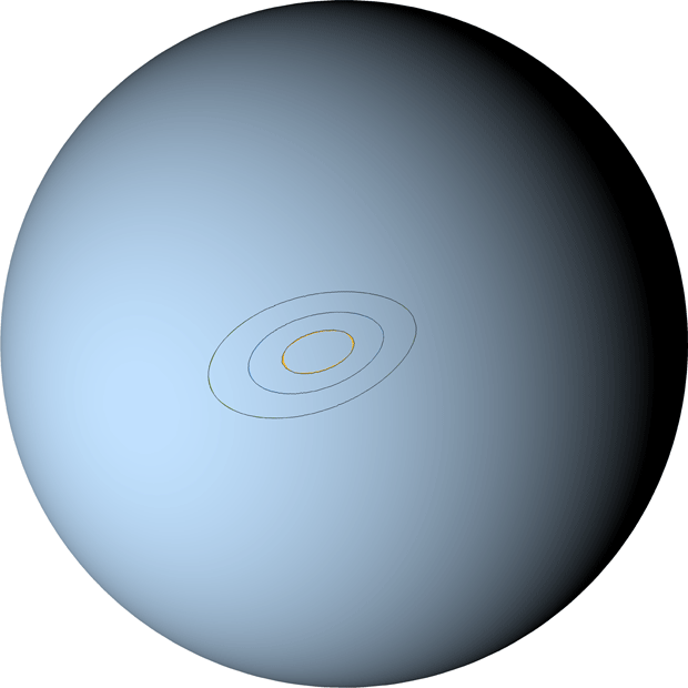
Depiction of the streamline pattern on the rotating sphere for the choice $f(z)=z^{2}+1$ and $a=1$ , $b\unicode[STIX]{x1D714}^{2}=2$ in (4.1).