


When do autocratic elites transfer power to excluded groups? Numerous theories of regime change and liberalization suggest that representation is granted in response to fears of social unrest. Yet, among such theories, there is disagreement as to whether the ability to produce such unrest—the disenfranchised group’s capacity for collective action—is more or less likely to produce institutional change.
The predominant view in the literature, expressed in various contributions that we discuss below, is that regime change and liberalization are more likely when excluded groups find it easier to overcome their collective-action problems. Intuitively, autocratic elites are vulnerable to social disturbances, so frequent unrest that poses a threat to regime stability should encourage institutional change. Yet, in a series of influential contributions, Acemoglu and Robinson (Reference Acemoglu and Robinson2000, Reference Acemoglu and Robinson2001, Reference Acemoglu and Robinson2006) argue precisely the opposite. In their theory, representation (democratization) is a commitment mechanism that is exploited only when the elite is otherwise unable to credibly commit to future redistribution—that is, when the majority poses an infrequent threat of unrest.
Existing empirical work on regime change does little to adjudicate this debate. To the extent that such work examines the relationship between unrest and representation, it typically focuses on whether democratization and other forms of regime change are more likely during periods of popular mobilization (Przeworski Reference Przeworski2009; Aidt and Jensen Reference Aidt and Jensen2014; Aidt and Franck Reference Aidt and Franck2015; Aidt and Leon Reference Aidt and Leon2016) or in the presence of adverse economic shocks (Brückner and Ciccone Reference Brückner and Ciccone2011).Footnote 1 Yet, if liberalization is more likely during such periods, so are redistribution, repression, and various other regime responses. The pertinent question is whether, at such moments, representation is more or less likely to be granted when an excluded group poses a more constant threat of unrest.Footnote 2 Answering this question requires that we have data on unrest before, not just when, institutional change occurs.
In this article, we exploit unique data and a novel empirical setting to explore the relationship between capacity for collective action and representation in autocracies. We focus on Russia during the period of the Great Reforms under Tsar Alexander II—an era in which the autocratic state emancipated the serfs and devolved substantial authority to previously excluded actors.Footnote 3 Key among these reforms was the creation (over most of European Russia) in 1864 of the zemstvo, an institution of local self-government with the authority to assess taxes and allocate revenues to local public goods, including healthcare and education. This authority was exercised by an elected assembly, with statutory allotments of seats for the gentry, urban property owners, and peasantry that varied greatly across 365 districts in which zemstva (pl.) were established. Nafziger (Reference Nafziger2011) demonstrates that these seat allotments were consequential for policy, with more spending on public goods and more taxation of the nobility where peasants had greater representation.Footnote 4
Our primary empirical exercise relates peasant representation in the district zemstvo assemblies to the frequency of peasant unrest from 1851 to 1863, which we assume to be correlated with perceptions of potential unrest at the time of reform—either because of persistence in underlying conditions or because previous conflict itself creates enduring capacity for collective action (Bellows and Miguel Reference Bellows and Miguel2009; Blattman Reference Blattman2009; Daly Reference Daly2012; Jha and Wilkinson Reference Jha and Wilkinson2012; Finkel Reference Finkel, Gehlbach and Olsen2015). To correct for measurement error in the unrest data and to support a causal interpretation of our results, we employ an instrumental-variables strategy that exploits two important and plausibly exogenous determinants of unrest in the pre-reform period: the historical incidence of serfdom (controlling for distance from Moscow, soil fertility, and the relative size of the rural/peasant population [serfs were just one of two major groups of peasants in Russia during this period], among other variables) and religious polarization.
Consistent with the Acemoglu-Robinson model of political transitions, and inconsistent with numerous other theories of regime change and liberalization, we find that peasants received less representation in zemstvo assemblies in districts that experienced more frequent peasant unrest in the years preceding 1864. Employing each instrumental variable in turn, we obtain generally similar results across a range of specifications, notwithstanding the fact that the two instruments capture largely distinct variation in peasant unrest.
Although these findings lend support to the Acemoglu-Robinson model, they do not speak directly to the commitment mechanism central to that theory. To explore causal mechanisms, we exploit a previously unrecognized empirical implication of the Acemoglu-Robinson framework: capacity for collective action should have a stronger, more positive impact on redistribution where representative institutions have not been granted. To test this prediction, we utilize new data on the expansion of rural Russian schooling—an important mode of redistribution—in the mid-nineteenth century. We find that the relationship between redistribution and unrest is in fact more negative in non-zemstvo districts—that is, those in which representative institutions do not serve as a commitment to future redistribution.
Our results suggest a puzzle. On the one hand, we find an impact of capacity for collective action on representation in autocracies that is consistent with the Acemoglu-Robinson model and inconsistent with many others. On the other, we observe a relationship between capacity for collective action and subsequent redistribution that is inconsistent with the commitment mechanism central to that model. Taken in total, our results are thus inconsistent with any existing model, suggesting the need for further theoretical work. We discuss possible directions for such work in the conclusion.
THEORETICAL PERSPECTIVES
The empirical exercise in this article is motivated by a substantial theoretical literature on the relationship between collective action and representation in autocracies. Our general approach is to lean on this work to the extent possible, resorting to post-hoc explanations only to the degree that we observe empirical patterns inconsistent with extant theory.
Beginning with the seminal work of Lipset (Reference Lipset1959), theories of regime change and political liberalization have emphasized a number of variables, including economic development, economic inequality, elite divisions, pacts, and popular mobilization. With respect to the last of these variables—the focus of this article—there is debate about the importance and even direction of any effect. On the one hand, social unrest may be epiphenomenal to other events driving transition. As Geddes (Reference Geddes1999) writes with respect to regime change in Latin America, “Popular mobilizations took place in many countries, but they usually occurred relatively late in the process, when democratization was well underway and the risks of opposition had diminished” (120). Similarly, Kotkin (Reference Kotkin2009) argues that elite attitudes rather than popular mobilization were the key reason for the collapse of communism in Eastern Europe in 1989.
On the other hand, the ability of political actors to exploit economic and other shocks may depend on their capacity for collective action, which elites in turn may anticipate. Among theories that suggest a causal effect of collective action on representation, most conclude that democratization or liberalization is more likely to occur when excluded groups find it comparatively easy to overcome their collective-action problems.Footnote 5 Collier (Reference Collier1999), for example, suggests that labor unions, with their inherent capacity for mobilization, play a critical role in the “destabilization and extrication” of nondemocratic regimes. Boix (Reference Boix2003), in turn, argues that greater mobilization among the poor or disadvantaged increases the likelihood of establishing a democratic state, though only when economic inequality is relatively low. Gandhi and Przeworski (Reference Gandhi and Przeworski2006) and Gehlbach and Keefer (Reference Gehlbach and Keefer2011) both predict that co-option (through the creation of legislatures and ruling parties, respectively) is more likely when the ability to suppress popular uprisings is small. Bueno de Mesquita (Reference Bueno de Mesquita2010) suggests that unrest fosters regime change by signaling widespread dissatisfaction with the incumbent regime. Besley, Persson, and Reynal-Querol (Reference Besley, Persson and Reynal-Querol2016) argue that political leaders with less “resilience,” which may be determined by the mobilizational capacity of excluded groups, are more likely to create institutionalized checks on the power of the executive branch.Footnote 6
A notable exception to this general consensus is the model of political transitions by Acemoglu and Robinson (Reference Acemoglu and Robinson2000, Reference Acemoglu and Robinson2001, Reference Acemoglu and Robinson2006). In their theory, representation (democratization) serves as a commitment mechanism for autocratic elites who are otherwise unable to commit to future redistribution, which is the case when the poor only occasionally pose a threat of unrest. The logic of the model is as follows. In any period in a nondemocracy, the poor pose a credible threat of revolution with probability q.Footnote 7 In such periods, the poor have “de facto political power,” which they can use to force concessions from the elite, who lose everything in a revolution. Ideally, the elite would prefer to minimize concessions by redistributing current income to the poor while retaining “de jure political power,” that is, the right to choose redistribution in future periods. When de facto political power is fleeting, however—when the poor only occasionally pose a credible threat of unrest (that is, when q is low)—then the poor anticipate that the elite will fail to redistribute in future periods. In this case, the only way the elite can credibly commit to future redistribution and, thus, prevent revolution is by transferring de jure political power to the poor, that is, by democratizing.
Acemoglu and Robinson (Reference Acemoglu and Robinson2000, 1185) illustrate the commitment mechanism with the following example: “At first sight, one might expect franchise extension in Germany [where unions and the socialist movement posed a nearly constant threat of unrest] rather than in Britain and France. Our model, in contrast, predicts that the German elite should have had more flexibility in dealing with social unrest by promising future redistribution, which was the pattern in practice.” In Appendix A, we show that this logic extends to a setting in which any level of representation (as opposed to democratization/not) can be chosen: the more frequently an excluded majority poses a credible threat of unrest (that is, the higher is q), the less representation the elite provides to the majority. We view this as the key empirical prediction of the Acemoglu-Robinson model—a prediction that has yet to be tested against other theoretical perspectives.
HISTORICAL CONTEXT
Our empirical analysis is grounded in the historical context of mid–nineteenth-century Imperial Russia. The period from 1850 to 1870 saw dramatic changes in the institutional structure of rural Russia as serfdom came to an end through a complicated set of reforms that helped usher in a new structure of governance in the countryside. In this section, we first describe the pertinent features of serfdom, the emancipation reforms, and their immediate impact on peasant unrest. We then delve into the origins and structure of the zemstvo’s system of representation.
Serfdom, emancipation, and peasant unrest
Russian serfdom was shaped by two interacting factors—the rulers’ need to maintain a large number of noble servitors, and the land/labor ratio (Domar Reference Domar1970). Noble service was compensated by land grants, but the availability of vast unsettled territories coupled with peasants’ freedom of movement threatened to put the nobility’s economic well-being at risk. To overcome this problem, the Muscovite state gradually introduced ever-increasing restrictions on the mobility of peasants. By the mid-seventeenth century, this led to the formalization of serfdom as a set of legal restrictions on the rights and freedoms of peasants residing on private estates.
Critically, serfs were but one part of the Russian peasantry. A slightly smaller group was the state peasants, who lived on state-owned land. By the mid-nineteenth century, state peasants were obligated only for rental payments to the state, possessed more labor autonomy and social mobility than did serfs, and could have private property of their own. While there were some differences in the geographic distribution of these two peasant groups, many provinces and districts had mixed populations. In addition, there was a relatively small population of court peasants, who lived on the lands owned by the royal family, and various other, less numerous groups classified as belonging to the peasant social estate.Footnote 8
During serfdom, the imperial government often confronted spasms of peasant violence, ranging from brutal murders of individual landowners to large-scale peasant uprisings, the most notable of which was the Pugachev Rebellion of 1773–75. Such unrest frequently necessitated military intervention, the cost of which was largely borne by the state rather than affected landowners. While serfdom and the hierarchical social-estate system laid the groundwork for these disturbances, other factors were also important. Religion played a key role in the functioning of the imperial state, with the regime co-opting Orthodox and non-Orthodox authorities to maintain social order. This strategy was most effective where there was a single large religious group, as religious leaders, laws, and customs were organically incorporated into the state apparatus. In contrast, where faiths intermingled, religions had to compete for their position in the state apparatus, leading to episodic conflict (Crews Reference Crews2003; Engelstein Reference Engelstein, Bermeo and Nord2000).
Over the first half of the nineteenth century, the Tsar’s fear of a backlash from the nobility prevented meaningful movement toward the elimination of serfdom. This position was no longer tenable in the wake of Russia’s defeat in the Crimean War (1853–56), which exposed Russia’s institutional backwardness and led to an increase in peasant unrest (Finkel, Gehlbach, and Olsen Reference Finkel, Gehlbach and Olsen2015). Although serfdom remained profitable for many landowners (Domar and Machina Reference Domar and Machina1984), fear of peasant rebellion encouraged Tsar Alexander II, who came to power during the war, to declare in 1856 that it was better to end serfdom “from above” than to wait for it to happen “from below.”
The Emancipation Manifesto and accompanying statutes of 1861 gave former serfs immediate legal freedom but fell far short of meeting their expectations with regard to land ownership. The reform’s content was a compromise between different factions of the elite over how much land, if any, should be awarded to the peasants (Khristoforov Reference Khristoforov2011, 9). The actual process of dividing rights to former estate land was largely delegated to the local nobility, who unsurprisingly took advantage of the opportunity to ensure that the resulting land deals were structured in their favor.Footnote 9 This resulted in renewed unrest across the Russian Empire: Finkel, Gehlbach, and Olsen (Reference Gandhi and Przeworski2015) document a sharp increase in disturbances among former serf peasants after 1861, versus a much smaller, statistically insignificant decrease among the nonserf peasant population. It was precisely in this period that a relatively small number of bureaucrats in St. Petersburg were occupied with drafting another reform, that of a new unit of rural self-government, the zemstvo. The timing was not coincidental: “The fundamental and decisive factor driving the [zemstvo] reform was the revolutionary situation in the country” (Garmiza Reference Garmiza1957, 42).
The zemstvo
In early 1864, Tsar Alexander II issued the Statutes on Provincial and District Zemstvo Institutions. This act established a new institution of local self-government—the zemstvo—in 34 of the 50 provinces of European Russia at both the provincial (guberniia) and district (uezd) levels (see Figure 1).Footnote 10 Although the original intention was eventual expansion across the empire, the initial law did not establish the zemstvo in more peripheral regions, including the Western borderlands under the local control of Polish Catholic nobility. Many of these regions were frequent sites of peasant unrest, as we discuss below, and they often possessed other forms of local or military governance.
The geography of the zemstvo as defined by the 1864 law. Zemstva were established in shaded districts. Dark lines indicate provincial boundaries. Three districts in black are not in the sample due to administrative reorganizations.

The founding statutes called on the zemstva to undertake programs to support “the local economic and welfare needs of each province,” and some fiscal authority was granted to enable such efforts. Annual assemblies approved spending and revenue policies under simple majority voting; these were then enacted by executive councils responsible for day-to-day operations. Nafziger (Reference Nafziger2011) documents a substantial increase in the provision of publicly provided local goods and services in zemstvo districts over the subsequent decades. Strikingly, this improvement was most pronounced in districts where peasants were granted greater (though typically minority, as discussed below) representation in the zemstvo assemblies, which likely reflected the greater ease in such districts of creating majority coalitions with progressive members of the nobility.
Under the 1864 law, between 10 and 100 assemblymen were to be elected for three-year terms in balloting by three groups, or curiae, of voters in each district: rural private-property owners (land-owning nobility), urban property owners, and peasant communes, which had gained formal status as parties to the emancipation reforms. Critically for our purposes, the statutes fixed the number of assembly seats from each curia in each district, with substantial variation according to “local and historical circumstances” (Komissiia o gubernskikh i uyezdnykh uchrezhdeniiakh 1890, 7). Under the 1864 law, the first curia (rural property owners) held 47% of all seats, versus 12.5% for the second curia (urban property owners), and 40.5% for the third curia (peasant communities).Footnote 11 When combined, the first and second curiae formed an overall statute majority in 323 of 365 districts in our sample. In contrast, the third curia held a plurality in 78 districts and an absolute majority in only eight (see Figure 2).
Share of zemstvo assembly seats statutorily assigned to third (peasant) curia c. 1875. Dark lines indicate provincial boundaries.

To understand the process by which these allocations were set and the possible role of peasant unrest in their formulation, it is important to reconstruct the specific historical context that generated the original 1864 statutes. Alexander II’s call for ending serfdom necessitated a reconsideration of how the countryside was to be governed, local taxes collected, and public goods provided (Komissiia o gubernskikh i uyezdnykh uchrezhdeniiakh 1890, 2). In March 1859, the Tsar appointed a special commission to decide the structure of local administration, led by the relatively liberal Deputy Minister of the Interior Nikolai Miliutin. In April 1860, the commission proposed that local public goods and services be provided by new “economic structures,” based on “elective principles” (Malloy Reference Malloy1969, 90). However, the details of these new bodies remained largely unspecified until after emancipation.
In April 1861, Alexander II reacted to noble fears amid growing rural unrest by replacing Miliutin with the conservative new Minister of the Interior, Petr Valuev (Garmiza Reference Garmiza1957, 154). From mid-1861 until mid-1863, the Valuev-led commission worked to define the parameters of the new structure’s electoral rules. As such, the specifics of the zemstvo reform were prepared exclusively in St. Petersburg and not by the provincial committees of nobility or other local bodies (ibid., ch. 2).Footnote 12 The commission, in turn, submitted an initial proposal to the State Council, which debated and modified the plan (in committee and then the full Council) in July and December 1863.
Revolutionary conditions, both in Poland and the Russian countryside, eventually encouraged the Council to establish property-based norms of representation to guarantee a leading role for the local land-owning gentry in the zemstvo assemblies. However, and notwithstanding these general criteria, it appears that the State Council also likely intervened to adjust district-level seat allotments on the margin, either directly or by tinkering with the amount of property in different categories to generate specific seat numbers once the general rules were applied. Unfortunately, detailed records of the Council’s deliberations are not preserved in the archives (Garmiza Reference Garmiza1957, 230–1). Our statistical analysis attempts to circumvent this break in the historical record by “reverse engineering” the seat allocations.
The St. Petersburg bureaucrats formulating the zemstvo reform had access to a wide range of expert commentary, alternative proposals, and information from local officials, individual nobles, and noble assemblies. The close connections between the larger peasant reforms and deliberations over the zemstvo law gave the commission data on the distribution of population by social class and rough estimates of the property holdings among different groups of owners. In addition, it is likely that the commission and the State Council had access to police reports on unrest in the countryside—probably with a lag, but certainly covering the period up to early 1863. These elements of the policymakers’ “information set” allowed them to consider a variety of factors, including the history of peasant unrest, in formulating the general rules and deviations therefrom governing the allocation of seats in the zemstvo assemblies.
EMPIRICAL STRATEGY AND DATA
We are interested in estimating the following model:
 $$\begin{equation}
\rho _{i} = \theta + q_i\zeta + {\rm Z}_i{\bm\mu }+\epsilon _i,
\end{equation}$$
where ρ
i
is our measure of political liberalization: peasant representation in the zemstvo assembly in district i, defined as percentage of seats allocated to the third (peasant) curia in the 1864 statutes. The variable q
i
is the frequency of potential unrest in district i, that is, the frequency with which the peasantry poses a threat to the nobility. (As the notation suggests, this variable is conceptually identical to the frequency q with which the excluded group poses a credible threat of unrest in the Acemoglu-Robinson model and in our extension thereto in Appendix A.) The associated coefficient ζ is our parameter of interest: the relationship between the capacity for collective action and representation. The variable θ is a constant, Z
i
is a vector of district-level covariates (described below) with parameter vector
 ${\bm \mu }$
, and ε
i
is an idiosyncratic error term.
The empirical challenge in estimating Equation (1) is that we do not observe the frequency q i with which the peasantry in district i poses a threat of unrest to the nobility, but rather the actual frequency of unrest in district i,
 $$\begin{equation}
\tilde{q}_i = q_i + \eta _i ,
\end{equation}$$
where η
i
is measurement error idiosyncratic to district i. Our measure of
 $\tilde{q}_i$
uses event-level data from Finkel, Gehlbach, and Olsen (Reference Finkel, Gehlbach and Olsen2015), who code a Soviet-era chronicle of peasant disturbances compiled during the Khrushchev Thaw (Okun’ Reference Okun’1962; Okun’ and Sivkov Reference Okun’ and Sivkov1963; Ivanov Reference Ivanov1964; Zaionchkovskii and Paina Reference Zaionchkovskii and Paina1968). In particular, we define
 $\tilde{q}_i$
as the proportion of years between 1851 and 1863, inclusive, for which these data record any disturbances:
 $$\begin{equation*}
\tilde{q}_i=\frac{1}{T}\sum _{t=1}^{T}d_{it},
\end{equation*}$$
where d it is an indicator that takes a value of one if there are any disturbances in district i in year t and T = 13. Figure 3 maps variation across districts in this measure of the frequency of unrest; Table 1 provides summary statistics for this and other variables.
Frequency of peasant unrest, 1851–1863. Dark lines indicate provincial boundaries.

Summary statistics

Note: Variables discussed and sources cited in the text.
We assume that previous unrest is informative of potential unrest at the time of reform, either because of persistence in underlying conditions or because unrest itself creates capacity for collective action through the acquisition of skills and repertoires (see the references above). Nonetheless, at least three considerations imply that
 $\tilde{q}_i \ne q_i$
. First, and most obviously, the chronicles on which the event data are based almost certainly underreport actual disturbances. At the same time, some reported disturbances may pose little real threat to the nobility. The empirical frequency of unrest
 $\tilde{q}_i$
may therefore be either an underestimate or overestimate of q
i
.
Second, the number of years T over which we aggregate disturbances may be either too small or too large. In principle, if q
i
is stationary, then
 $\tilde{q}_i$
will be a better estimate of q
i
when T is large, that is, when the time series is long. In practice, observations of unrest closer to the period in which representation is chosen are likely to be more informative (or salient) to policymakers, given that the threat of unrest may change over time. One could view our choice of T = 13, which corresponds to the period from 1851 (the first year in the dataset) to 1863 (the year before reform), as a plausible middle ground between these two considerations.
Third, before establishment of the zemstva, landowners may have responded to the threat of unrest by providing local concessions, thus dampening actual disturbances d it . In practice, the incentives for decentralized reform of this sort were limited, given that the local nobility did not fully internalize the cost of unrest, largely because the central state bore the cost of calling out military detachments. Nonetheless, to the extent that any such tendency was greater in regions with a higher baseline threat of unrest, then the variable q i will be correlated with the measurement error η i .
As this discussion illustrates, both classical and (potentially) nonclassical measurement error complicate the estimation of Equation (1). To address this issue, as well as concerns about simultaneity or omitted-variable bias, we use instrumental variables. We draw upon the historiography of Imperial Russia to select instruments that not only meet the usual criteria (strength in the first stage and excludability relative to Equation (1), of which more below) but also drive variation in unrest in a way that was likely understood by the bureaucrats who set the statutory allocations for zemstvo assemblies—an additional consideration that lends support to a causal interpretation of our results.
Our first instrument for
 $\tilde{q}_i$
is the historical incidence of serfdom, which we define as the proportion of serfs in the district population in 1858 using data from Troinitskii (Reference Troinitskii1861) and Bushen (Reference Bushen1863).Footnote
13
As discussed above, serfdom was associated with a greater incidence of unrest throughout the 1850s and early 1860s, a relationship that seems to have been foremost in the minds of the bureaucrats who set the statutory allocations of seats in district zemstvo assemblies.
Geographic variation in serfdom was substantially determined by a district’s distance from Moscow (and thus from St. Petersburg, the subsequent imperial capital)—a legacy of the territorial expansion of the Muscovite state, as military service was rewarded by grants of land to the nobility—and by the suitability of land for agricultural production, each of which might have independently affected peasant representation. To partial out these effects, we condition on distance from Moscow and a measure of fertile soil constructed from GIS-coded data on soil type from the Food and Agriculture Organization (FAO).Footnote 14 We also control for a variety of other district characteristics that are plausibly correlated with both the instrument and peasant representation. As discussed above, representation in the various curiae was determined in part by the property holdings—in the countryside, highly correlated with number of peasants—of urban and rural landholders. Although the formulae that governed these relationships were themselves the outcome of political contestation, we include the logs of urban population and total population (and thus, implicitly, urbanization),Footnote 15 from Tsentral’nyi statisticheskii komitet (1866; the data refer to 1863), to isolate the effect of unrest on representation. In particular, the population controls implicitly condition on the relative size of the rural/peasant population and thus capture any interest in restricting peasant (as opposed to specifically serf) representation in the zemstvo assemblies. Finally, we condition on whether the district hosts a provincial capital, as such cities were more likely to have their own quasi-representative legislative assemblies, perhaps limiting the need for representation of the masses.
After conditioning on these covariates, we are left with that portion of serfdom largely determined by idiosyncratic variation in land grants to the nobility decades or centuries before the zemstvo reform of 1864.Footnote 16 Our identifying assumption is that such variation is uncorrelated with the error term ε i in Equation 1 and the measurement error η i in Equation 2. With respect to the latter part of this assumption, below we report results in which we systematically exclude classes of events that, in principle, could have entered the archives with greater or lesser frequency in districts where serfdom was predominant.
As a second instrument for the frequency of unrest, we employ a measure of religious polarization, defined in the standard way for district i as
 $$\begin{equation*}
4\sum _{r\in R} \pi _{ri}^2\left(1-\pi _{ri}\right),
\end{equation*}$$
where r indexes religious affiliations and the set R includes Orthodox, Schismatic (Old Believer), Armenian Gregorian (Armenian Apostolic), Catholic, Protestant, Jewish, Muslim, and Idolator—the eight categories defined in population data published shortly after the zemstvo reform (Tsentral’nyi statisticheskii komitet 1870).Footnote 17 A substantial literature ties ethnic and religious polarization to conflict (e.g., Esteban and Ray Reference Esteban and Ray1994, Reference Esteban and Ray2008; Montalvo and Reynal-Querol Reference Montalvo and Reynal-Querol2003, Reference Montalvo and Reynal-Querol2005; Mitra and Ray Reference Mitra and Ray2014.).Footnote 18 In our empirical setting, as discussed above, unrest was provoked not only by cultural difference but by the inability of religious authorities to maintain social order as part of the state apparatus in areas with sizable religious minorities. As Figure 4 illustrates, the potential for conflict was generally most pronounced in outlying regions, where non-Orthodox religious groups were concentrated—a pattern that was well understood by imperial authorities.
Historical prevalence of serfdom and religious polarization. Dark lines indicate provincial boundaries. The first map illustrates the legacy of territorial expansion of the Muscovite state.

As with serfdom, the excludability of religious polarization relies on controlling for the various district characteristics discussed above; distance to Moscow is particularly important, given the historical settlement patterns of various religious groups. After controlling for these covariates, the pairwise correlation between the incidence of serfdom and religious polarization is −0.09. Thus, the two instruments pick up largely distinct variation in our measure of peasant unrest, so that the estimates from our two sets of instrumental-variables regressions represent different local average treatment effects.
RESULTS
Before presenting our estimation results, we examine the decision to grant representative institutions to various regions in European Russia—that is, whether to have zemstva at all. With one exception—Ismail’skii district in Bessarabiia—such selection occurred at the provincial rather than district level, for various reasons discussed above, including Polish dominance in the Western borderlands and the presence of alternative forms of local or military governance. A Heckman-type strategy to correct for potential selection bias is therefore equivalent to a regression with provincial fixed effects (Semykina and Wooldridge Reference Semykina and Wooldridge2010), results for which we present below. Nonetheless, it is instructive to examine the relationship between unrest and whether provinces were selected to receive zemstva. Conditioning on the various covariates discussed above, we find that zemstva are less likely to be created in provinces with more unrest, though only when instrumenting unrest on either serfdom or religious polarization.Footnote 19
We proceed to examine the relationship between collective action and peasant representation among those districts that did receive zemstva. Column 1 of Table 2 presents results from a “naive” OLS regression (that is, ignoring the sources of potential measurement error discussed above) of peasant representation in the district zemstvo assemblies on the observed frequency of peasant unrest from 1851 to 1863 and covariates. Consistent with a commitment theory of institutional change, and inconsistent with many other theories of collective action and liberalization, we find a negative relationship between peasant unrest and the statutory allocation of district zemstvo assembly seats to peasant communities in 1864. The point estimate, however, is not large: a district with frequency of unrest in the 25th percentile would lose approximately one percentage point of representation (relative to a mean of 41%) if it instead had frequency of unrest in the 75th percentile.
Peasant representation and unrest: OLS and IV (serfdom)

Notes: The dependent variable is percentage of seats statutorily allocated to peasant communities in the district zemstvo assembly. The pre-reform proportion of serfs in the district population is used as an instrument in the models in Columns 2–8. The model in Column 6 includes provincial fixed effects. Column 7 is an IV model with spatial autoregressive disturbances, implemented using spivreg in Stata, that uses an inverse-distance spatial weighting matrix. The sample in all regressions is 365 districts in European Russia. Heteroskedasticity-robust standard errors for all specifications (including Column 7) in parentheses. Kleibergen-Paap rk Wald F-statistic reported for first-stage F-stat. Significance levels: *** = 0.01, ** = 0.05, * = 0.10.
As discussed above, various forms of measurement error imply that OLS regression does not provide a credible estimate of the effect of unrest on representation. We therefore turn to instrumental-variables regression. In Column 2, we instrument frequency of unrest with the prevalence of serfdom in 1858. The first-stage F-statistic is quite large, reflecting the strong correlation between the instrument and the potentially endogenous variable: a one-standard-deviation increase in the historical incidence of serfdom is associated with a very precisely estimated 0.4-standard-deviation increase in the frequency of unrest.Footnote 20 The estimated effect of unrest in the second stage, in turn, is negative, precisely estimated, and substantially larger than that in Column 1. The difference in magnitude across the two estimates is consistent with attenuation bias resulting from measurement error—observe in particular that nonclassical measurement error of the sort discussed in the previous section could substantially flatten the OLS estimate—and also potentially related to the fact that the IV estimates represent local average treatment effects.Footnote 21 Fixing controls at their median values, the point estimate implies that, were a district to experience an increase in unrest from the 25th to the 75th percentile, peasant representation would decrease from 48.3 percentage points—nearly a simple majority—to just 38.5 percentage points.
The historical experience of a few informative cases helps to illustrate the negative relationship between unrest and representation. (We present the logic behind our selection of these cases in the online appendix.) In the Solikamskii district of Perm’ province, the authorities went out of their way to ensure the nobility’s domination in the zemstvo, to the point of granting the small number of land-owning gentry more seats than there were eligible nobles in the district (Larionova Reference Larionova2013). On the other hand, in the Iadrinskii and Koz’modem’ianskii districts of Kazan’ province (contemporary Chuvashiia), where there were similar numbers of eligible nobles, the authorities allowed the peasants to dominate the local zemstvo. The difference in outcomes is plausibly driven by different histories of peasant unrest. Solikamskii and neighboring Permskii district had a history of large-scale peasant mobilization—conditioning on covariates, these are the most turbulent districts in our sample. In contrast, authorities in largely peaceful Chuvashiia did not perceive peasants as a threat, viewing the few disturbances that did take place as a result of “misunderstandings . . .[and] not political resistance” (Ialtaev Reference Ialtaev2012, 44).
Error in measuring the underlying frequency of potential unrest may be driven in part by the inclusion of less consequential disturbances in our unrest data. Although acts of quotidian resistance—the “weapons of the weak” that James Scott describes (Scott Reference Scott1985)—are generally unlikely to have entered our data, as a check on our results, we recalculate the frequency of unrest using only events that spanned multiple villages or districts.Footnote 22 As examples, consider the following events, which are drawn from the chronicles on which our data are based. In March–April 1861, more than 17,000 peasants demonstrated in three districts of Perm’ province against the terms of emancipation. The military was called out and a number of peasants were shot by soldiers in the village of Egva. In June 1862, close to 300 peasants in three villages of Petersburg province refused to fulfill their labor obligations and disobeyed local authorities, prompting a military response. And in February 1863, a thousand peasants in two villages in Poltava province refused to pay quitrent and liberated their arrested ringleaders; once again, troops put down the unrest. The estimates in Column 3 demonstrate that our results are robust to defining unrest as such “large” events. Indeed, in standardized terms, the estimated effect of unrest is quite similar to that from the baseline IV model in Column 2, as Figure 5 illustrates.Footnote 23
Comparison of instrumental-variables estimates. The figure depicts the estimated effect of a one-standard-deviation increase in peasant unrest (defined variously) on peasant representation in district zemstvo assemblies. Markers indicate point estimates, lines 90% confidence intervals.

As discussed above, a key identifying assumption is that measurement error in the unrest variable is uncorrelated with the instrument, after conditioning on covariates. This assumption would be violated if the presence of “peace arbitrators” or other officials assigned to facilitate post-emancipation settlements between landowners and former serfs (Easley Reference Easley2008) resulted in more reporting of unrest in former serf areas. We check for this possibility in various ways. First, as shown in Column 4, we restrict attention to events drawn from the archive TsGAOR (Central State Archive of the October Revolution, currently a part of the State Archive of the Russian Federation), which primarily includes reports of the Imperial secret police and excludes reports of provincial governors, through which accounts of unrest by peace arbitrators would likely have passed. Second, as shown in Column 5, we restrict attention to disturbances during the pre-emancipation period. Our finding of a large, negative effect of unrest on peasant representation is robust to these manipulations—indeed, in standardized terms, the point estimate is somewhat larger using the latter definition of unrest, as depicted in Figure 5.
The results reported above assume that there is no unobserved spatial dependence among districts. The regressions in Columns 6 and 7 relax this assumption. In Column 6, we include province fixed effects; the estimated effect on peasant representation of capacity for collective action is slightly larger than that in the baseline model of Column 2. In Column 7, in contrast, we estimate an instrumental-variables model with spatial autoregressive disturbances (implemented with the spivreg command in Stata) using an inverse-distance spatial weighting matrix. The point estimate of the coefficient on the frequency of unrest is somewhat smaller than when we assume spatial independence, but it is still substantively large and statistically significant. As shown in the online appendix (Table A4), we obtain almost identical results if we instead employ a contiguity matrix that assigns a value of one to immediate neighbors (only). Similarly, the estimated effect of unrest is almost identical to that in Column 2 when we condition on latitude, longitude, and their squares (again, Table A4).
With respect to covariates, distance from Moscow is negatively correlated with peasant representation in all IV specifications, potentially reflecting fear of unrest close to the imperial center (Campante and Do Reference Campante and Do2009). The positive conditional correlation of soil fertility with representation—significant in most specifications—may represent the relationship between soil fertility and the (unobserved) evolved pattern of land ownership, which could have influenced representation through the property-based norms of representation discussed above.Footnote 24 The negative estimated effect of urban population (and thus, urbanization, given the log transformation of the population variables) is consistent with the formulaic allocation of seats to the second curia. (As shown in Table A4 in the online appendix, our results are very similar if we exclude Moscow and St. Petersburg, by far the two most urban and populous districts, from the sample.) The negative estimated coefficient on our dummy for “provincial capital” can be explained similarly.
In Column 8 of Table 2, we re-examine the excludability of serfdom as an instrument. Even relatively liberal administrators felt that peasant illiteracy and political inexperience necessitated overrepresentation by the nobility in zemstvo assemblies. To the extent that such fears were directed at former serfs in particular, as opposed to the peasantry in general—as discussed above, our empirical strategy implicitly conditions on the relative size of the rural/peasant population—this would suggest an impact of serfdom on representation other than through unrest. Our reading of the historical record suggests this was not the case. To the contrary, the peasantry, which also included state and court peasants, was seen by the government as a monolithic group with similar attributes and desires (Komissia o gubernskih i uyezdnykh uchrezhdeniakh 1890, 12). Nonetheless, as an additional check, we can proxy for (potentially observable) skills useful for governance with the number of rural schools circa 1860.Footnote 25 There were indeed fewer rural schools per capita in districts where serfdom was prevalent, but the estimated effect of unrest on representation is very similar when conditioning on the (log of) rural schools (+1). We explore the relationship between capacity for collective action and subsequent spending on rural education further below.Footnote 26
As an additional check on our results, we run the reduced-form (OLS) regression with serfdom in the covariate vector: see Column 9. Serfdom is strongly correlated with peasant representation, with an estimated coefficient that is significantly different from zero at p = 0.01. An increase over the whole range of serfdom (from 0 to 0.852) is associated with a decrease in peasant representation of approximately one-fifth of the range of the latter variable—a plausible magnitude, though we do not have strong priors about the size of any relationship. As we discuss below, the reduced-form regression can be even more useful in the context of weak instruments.
In addition to the numerous robustness checks reported above, we show in the online appendix that our results are robust to various other changes in measurement, specification, and sample. In principle, for example, income fluctuations caused by weather shocks could generate peasant unrest in the pre-reform period that reformers did not expect to persist, thus threatening our assumption that perceptions of potential unrest are correlated with prior unrest. In practice, the history of such income fluctuations may be largely absorbed by the spatial controls discussed above. As an additional check, we use province-level panel data on rye prices as a proxy for weather shocks. Consistent with the idea that weather shocks are reflected in grain prices, and that income fluctuations drive unrest, we find that unrest is greater when rye prices are high. Nonetheless, after purging our unrest variable of this relationship, the estimated effect of unrest on representation is negative, as before (see Table A6).
In addition, our results are very similar if we drop the 22 districts (out of 365) with zero reported disturbances from 1851 to 1863 (Table A5). We also obtain similar results if we give greater weight to disturbances temporally proximate to 1864 (Table A5). Including a quadratic term for frequency of unrest demonstrates a negative effect of unrest on representation for all but the upper quintile of unrest (Table A5). Finally, although peasant representation is not “censored” in the usual sense of the term—representation is theoretically bounded at zero and, in practice, peasants received nontrivial representation wherever zemstva were created—we obtain similar results from a Tobit model in which we code non-zemstvo districts as having zero peasant representation (Table A1). We conclude that the finding of a negative relationship between unrest and representation is quite robust.
Table 3 presents results of regressions that employ our second instrument, religious polarization. Looking across the columns of the table, we see a consistently negative estimated effect of frequency of unrest on peasant representation. Although the standard errors are substantially larger than for the corresponding regression in Table 2, reflecting the generally weaker correlation between unrest and religious polarization (as reflected in first-stage F-statistics, especially for the specification with provincial fixed effects),Footnote 27 the estimated magnitude is typically similar to that when serfdom is instead used as an instrument, as illustrated by Figure 5.Footnote 28
Peasant representation and unrest: IV (religious polarization)

Notes: The dependent variable is percentage of seats statutorily allocated to peasant communities in the district zemstvo assembly. Religious polarization is used as an instrument in all models. The model in Column 5 includes provincial fixed effects. Column 6 is an IV model with spatial autoregressive disturbances, implemented using spivreg in Stata, that uses an inverse-distance spatial weighting matrix. The sample in all regressions is 361 districts in European Russia. Heteroskedasticity-robust standard errors for all specifications (including Column 6) in parentheses. Kleibergen-Paap rk Wald F-statistic reported for first-stage F-stat. Significance levels: *** = 0.01, ** = 0.05, * = 0.10.
The reduced-form results in Column 8 of Table 3 provide additional evidence of a nonzero effect of unrest on representation. As Chernozhukov and Hansen (Reference Chernozhukov and Hansen2008) demonstrate, under the assumption that the instrument is excludable, the null hypothesis that the endogenous variable has zero effect can be rejected if the estimated coefficient on the instrument in the reduced-form regression is significantly different from zero—even if the instrument is weakly correlated with the endogenous variable, as is true here.
As reported in the online appendix (Tables A5, A6, A8, and A9), the results in Table 3 are robust to the numerous changes in sample and specification discussed above with respect to Table 2, though the effect of unrest in these exercises is not always precisely estimated—not surprising, given the relative weakness of the polarization instrument.Footnote 29 As an additional check, we also re-examine the excludability of religious polarization as an instrument. In principle, the religious (and thus ethnic) composition of the local population could affect representation in the district zemstvo assemblies directly—for example, if there were a greater willingness to grant peasant representation when the local population was predominantly Orthodox. (Although there is evidence that the state worked equally with all religious groups [Crews Reference Crews2003], Orthodoxy was one of the three elements of the “official nationality” promulgated under Alexander II’s father, Tsar Nicholas I—the other two being autocracy and nationality [narodnost’]; see, for example, Riasanovsky Reference Riasanovsky1959, 78.) If this were the case, such an effect would run through the share of the local population that was Orthodox, which is related to but distinct from our measure of religious polarization.Footnote 30 In Column 7 of Table 3, we include the share of the local population that is Orthodox.Footnote 31 Although the high correlation between this variable and religious polarization (r = −0.87) results in a substantial loss of instrument strength, the point estimate on frequency of unrest is qualitatively similar to (in fact, larger than) that in the baseline model.
UNREST AND REDISTRIBUTION
The finding that peasant representation in district zemstvo assemblies is negatively associated with capacity for collective action among the peasantry is consistent with the Acemoglu-Robinson model of political transitions and inconsistent with numerous other models. Yet our results could also be consistent with unmodeled rationales for not providing representation to groups with capacity for collective action. To examine this possibility, we explore a previously unrecognized implication of the commitment mechanism in the Acemoglu-Robinson model that does not obviously follow from other theories.
Holding representation constant, we expect more redistribution to excluded groups that have greater capacity for collective action—this is the logic of buying off those who threaten rebellion. At the same time, when representation is granted as a commitment device, less representation is provided to groups that have greater capacity for collective action, thus reducing their ability to bargain for redistribution through representative institutions. Conditional on some representation having been granted, these two effects offset each other—precisely so, if we assume no deadweight loss from taxation, though this is not essential to our main empirical analysis. In contrast, when no representation has been granted, only the first effect operates. If representation serves as a commitment device, we should therefore observe a stronger, more positive relationship between redistribution and capacity for collective action when no representation has been granted. We formalize this intuition in Appendix B, using the extension to the Acemoglu-Robinson model discussed above.
To test this prediction, we examine the relationship between capacity for collective action and redistribution in districts with and without zemstva. Doing so requires that we have data on redistribution over an extended period of time, during years when peasant unrest was a greater or lesser threat. Although panel data on redistributive expenditures are unavailable for this period, we can exploit data on the number of rural schools created between 1860 and 1880 (see below), which capture the ebbs and flows of local education spending by various authorities during the decades following the zemstvo reform.Footnote 32
Spending on rural schools in late Imperial Russia was clearly redistributive (Nafziger Reference Nafziger2012). Nonetheless, there were other major categories of redistributive spending during this period—especially healthcare (Frieden Reference Finkel, Gehlbach and Olsen1981)—which complicates our ability to infer overall redistribution from one of its components. In particular, the incentive to spend on education versus other priorities likely depended on the outstanding need for such spending—less incentive to build schools where they existed prior to reform, more where alternative needs were already satisfied.
To address this issue, consider the following simple model. Assume that the total budget available for spending on redistributive goods is x. We are interested in inferring x from observed data on education spending s and the initial stock of school spending
 $\bar{s}$
. (In our empirical exercise, s,
 $\bar{s}$
, and thus x are denominated in rural schools per capita.) Any portion of x not devoted to s is devoted to an alternative use (e.g., healthcare), where the unobserved initial stock of spending on that use is u. We assume that the division of x into education and other spending is governed by a social-welfare function that takes the Cobb-Douglas form:
 $$\begin{equation*}
\left(s + \bar{s}\right)^{\alpha }\left(x-s+u\right)^{1-\alpha },
\end{equation*}$$
where α is the preference weight placed on education versus other uses. Subjecting this function to a log transformation and maximizing the resulting expression with respect to s gives the first-order condition
 $$\begin{equation*}
\frac{\alpha }{s^{\ast }+\bar{s}}-\frac{1-\alpha }{x-s^{\ast }+u}=0,
\end{equation*}$$
where s* is the optimal level of education spending. We can use this expression to back out x as
 $$\begin{equation}
x=\left(\frac{1-\alpha }{\alpha }\right)\left(s^{\ast }+\bar{s}\right)+s^{\ast }-u.
\end{equation}$$
Total spending on redistributive goods is thus a function of observed post-reform education spending s* and the initial stock of education spending
 $\bar{s}$
, an unobserved preference parameter α, and an idiosyncratic component u.
To operationalize this expression, we define
 $\bar{s}$
as the number of rural schools in 1860, the first year prior to the zemstvo reform for which this variable is available (compiled from information reported in Fal’bork and Charnoluskii, eds., 1900-1905), and s* as the change in number of rural schools from 1860 to 1880, using the previous variable and a count of the number of rural schools in 1880 (Tsentral’nyi statisticheskii komitet 1884). We normalize both variables by the size of the rural population in 1883 (in thousands), the closest available data to 1880.Footnote
33
As we do not observe α, we check the robustness of our results to a range of assumptions about the value of this parameter. Realized education spending comprised 16% of all zemstvo expenditures in 1883, and approximately 39% of the total of education and medical expenditures (Nafziger Reference Nafziger2011). As such, we estimate models with α = 0.10, 0.25, and 0.50. (Observe that the idiosyncratic component u in Equation (3) is absorbed by the error term in any regression with x as the dependent variable.) As we show in the online appendix (Table A11), both our qualitative findings and the statistical significance of our estimates are robust to the choice of α. To economize on space, we report results here for α = 0.25.
We thus proceed to estimate the relationship between redistribution and capacity for collective action in districts with and without zemstva. We begin by “naively” defining redistribution as the change in the number of rural schools from 1860 to 1880, normalized by rural population in 1883. To correct for measurement error in capacity for collective action, we instrument frequency of unrest (measured from 1851 to 1863) and its interaction with non-zemstvo status with our measure of serfdom and its interaction with the same dummy variable. As discussed above, the commitment mechanism central to the Acemoglu-Robinson model suggests a stronger, more positive effect of capacity for collective action on redistribution in non-zemstvo regions. The results in Column 1 of Table 4 show that we find precisely the opposite relationship.
Unrest and redistribution

Notes: The dependent variable in Columns 1, 3, 5, and 7 is the change in number of rural schools from 1860 to 1880, normalized by rural population in 1883. The dependent variable in Columns 2, 4, 6, and 8 is redistribution, defined using the Cobb-Douglas procedure described in the text for α = 0.25. The pre-reform proportion of serfs in the district population and its interaction with an indicator for no zemstvo are used as instruments in all models. Frequency of unrest is calculated using data from 1851–63 (that is, before creation of the zemstvo) for all columns but Columns 7–8, which use 1851–60. Heteroskedasticity-robust standard errors for all specifications in parentheses. Kleibergen-Paap rk Wald F-statistic reported for first-stage F-stat. Significance levels: *** = 0.01, ** = 0.05, * = 0.10. For all regressions, 488 observations, of which 365 with zemstva.
The second column of Table 4 presents results for a model in which redistribution is defined using our Cobb-Douglas approach. As before, capacity for collective action is more negatively associated with redistribution in non-zemstvo regions: precisely the opposite of what we would expect if representation were chosen optimally as a commitment device. The remaining columns show that this result holds for the various alternative measures of unrest used in Tables 2 and 3.
In addition to the main implication of the commitment mechanism in the Acemoglu-Robinson model tested here, our formalization generates two subsidiary empirical predictions. First, as discussed above, when there is no deadweight loss from taxation—a special case—there should be no relationship between redistribution and capacity for collective action, conditional on some representation having been granted. Table 4 demonstrates mixed evidence in support of this prediction, with an estimated coefficient on frequency of unrest that is not significantly different from zero only when defining redistribution as change in the number of rural schools. Second, as shown in Appendix B, when representation serves as a commitment device, the “level effect” of being in a district with no representation (that is, no zemstvo) should be negative; we find precisely the opposite.
As shown in the online appendix (Table A12), the negative interaction between frequency of unrest and non-zemstvo status is robust to excluding all districts in Orenburg, Astrakhan, and Arkhangel’sk, plus the Ismail’skii district in Bessarabia, thus leaving the contiguous districts in right-bank Ukraine, Belorussia, and the Baltics in the non-zemstvo set. Our results are also similar if we split the sample rather than assume an effect of covariates that is constant across zemstvo and non-zemstvo regions. Finally, although the first stage is weaker and second-stage estimates correspondingly less precise, we obtain similar qualitative results, presented in the online appendix (Table A11), when using religious polarization and its interaction with the non-zemstvo indicator as instruments.
Taken together, our findings are not explained by existing models. Consistent with the Acemoglu-Robinson model of political transitions, we find that less representation is granted when the excluded group has greater capacity for collective action. But a further implication of that model—that we should find a stronger, more positive effect of capacity for collective action on redistribution in districts where no representation is granted—finds no support. We are left to infer the presence of some theoretical mechanism not reflected in existing models of liberalization and regime change.
CONCLUSIONS
We examine the statutory assignment of seat shares in institutions of local self-government created in Russia during the period of the Great Reforms under Tsar Alexander II. We find that political representation was less likely to be granted to peasants who posed a more persistent threat of unrest. Our instrumental-variable estimates, which correct for measurement error in the unrest data, suggest a causal interpretation: capacity for collective action induced by idiosyncratic variation in the historical prevalence of serfdom and religious polarization decreased peasant representation.
Among various theoretical models of institutional change, these results are most consistent with the Acemoglu-Robinson model of political transitions (Acemoglu and Robinson Reference Acemoglu and Robinson2000, Reference Acemoglu and Robinson2001, Reference Acemoglu and Robinson2006), which predicts that representation is less likely to be granted when elites are otherwise able to commit to future redistribution—that is, when excluded groups pose a persistent threat of unrest. Yet, our subsequent analysis of post-reform redistribution finds a relationship with unrest that is inconsistent with this commitment mechanism.
What might account for the negative effect of unrest on representation that we observe in our data, if not a greater ability to commit to groups that pose a more frequent threat of rebellion? One possibility is a simple punishment story: peasants who pose a more frequent threat of unrest are punished with less representation. This is a tempting explanation—one that at an abstract level is plausibly supported by the theory of reputations and repeated games. But it is worth emphasizing that the “punishment” imposed by imperial authorities was particularly “grim”—the allocation of seats did not change after 1864 until 1890, at which point peasants received fewer seats. Moreover, a strategy of building or sustaining a reputation for toughness seems at odds with the basic decision to create institutions of local self-government.
More plausible, in our view, is that Russian officials provided little representation to peasants with a history of rebellion in the interests of demobilization. In the typical model of regime change or liberalization, reform serves to discourage rebellion. In the Russian context, in contrast, reformers may have feared that providing representation to rebelling peasants would simply fan the flames—say, because peasants now had access to the machinery of the state.Footnote 34 Such fears would have been informed by recent experience, as emancipation of the serfs in 1861 led to increased unrest across the Russian countryside. Consistent with this perspective, Starr (Reference Starr1972) writes that Russian Interior Minister Petr Valuev reacted to unrest in the early 1860s by seeking “to bar ‘communists and men of low morality’ from the zemstvos” (247).
Finally, and not mutually inconsistently, the allocation of seats may have been driven by concerns about moral hazard. Much of the cost of putting down rebellion in the Russian countryside was borne not by landowners but by the central state. Providing more representation to local elites in districts with a history of unrest may have been a way of incentivizing those elites to keep rebellion under control.
Fully exploring these alternative theoretical mechanisms—their internal consistency and their application to other empirical contexts—is a task for future research.
APPENDIX A: A GENERALIZATION OF THE ACEMOGLU-ROBINSON MODEL
In this section, we present a simple adaptation of the Acemoglu-Robinson model of political transitions that allows for a continuous institutional choice by the elite, as in the empirical setting that we study. As we show, the key empirical implication of the model is qualitatively similar to that of the Acemoglu-Robinson model: the elite liberalizes less when the excluded group more frequently poses a threat of unrest.
Environment
The model is a Markov game in which in each period of the political regime is either unliberalized (U) or liberalized (L). There is an elite (E) and an initially excluded majority (M), which we treat as unitary actors. In an unliberalized regime, the elite has full control rights over policy. In a liberalized regime, control rights are divided between the elite and majority according to a process described below.
At issue is the distribution of income between the elite and majority. For reasons of parsimony, we abstract from the initial distribution of income, focusing instead on a simple divide-the-pie environment (as in Gehlbach Reference Gehlbach2013, Section 8.4.1). In particular, in any period t, whoever has control rights over policy names a division x t of an infinitely divisible resource of size one, where x t is the portion of the resource received by the majority; the remainder 1 − x t is received by the elite. We assume that the majority and elite receive payoffs from this distribution equal to x t and 1 − x t , respectively. In what follows, we suppress the subscript t for notational simplicity.
Regardless of whether the political regime is liberalized, in any period the majority decides whether to revolt after observing the policy choice x. The cost of revolution is given by the random variable μ ∈ {κ, 1}, which is realized prior to choice of policy x and observed by both elite and majority. We assume κ ∈ (0, 1), with
 $\Pr (\mu =\kappa )=q$
. If the majority revolts, the state immediately transitions to the absorbing state (R, μ). In this state, in any period the majority receives payoff 1 − μ, whereas the elite receives payoff 0. (As in the Acemoglu-Robinson model, the natural interpretation is that the economy suffers a permanent productivity shock from revolution.) Thus, revolution is attractive to the majority only if μ = κ.
Up to this point, the game is essentially identical to the basic Acemoglu-Robinson model but for the stylization of the economic environment. In a departure from the Acemoglu-Robinson framework, we assume that the elite can liberalize by adopting any level of majority representation ρ ∈ (0, 1). The variable ρ determines who has control rights over policy in a liberalized regime. In particular, in any period, after realization of μ, the random variable α ∈ (e, m) is realized, where
 $\Pr (\alpha =m)=\rho$
. If α = e, the elite chooses policy in the current period, whereas if α = m the majority does.
To summarize, the state space in a liberalized regime is
 $$\begin{equation*}
\left\lbrace \left(L,\kappa ,m\right),\left(L,\kappa ,e\right),\left(L,1,m\right),\left(L,1,e\right)\right\rbrace ,
\end{equation*}$$
whereas that in an unliberalized regime is {(U, κ), (U, 1)}. In a liberalized regime, following realization of the random variables μ and α, whoever has control rights over policy (elite or majority, depending on α) names a distribution x, following which the majority decides whether to revolt. In an unliberalized regime, following realization of the random variable μ, the elite decides to liberalize or not. If the elite chooses not to liberalize, it subsequently names a distribution x, following which the majority decides whether to revolt. In contrast, if the elite chooses to liberalize, the random variable α is realized, following which the game proceeds as in any period in which the regime is liberalized. In particular, the value of the random variable μ “inherited” from the unliberalized regime persists until the start of the next period.
Players discount payoffs by the common discount factor δ ∈ (0, 1).
Equilibrium
We solve for a Markov perfect equilibrium, where players’ strategies are conditioned only on the current state. We begin by analyzing behavior in the unliberalized regime, given that the elite chooses not to liberalize. Writing down the Bellman equation for the majority for each of the two possible states gives
 $$\begin{eqnarray*}
V_{M}\left(U,\kappa \right) & = & \hat{x}+\delta \left[qV_{M}\left(U,\kappa \right)+\left(1-q\right)V_{M}\left(U,1\right)\right],\\
V_{M}\left(U,1\right) & = & 0+\delta \left[qV_{M}\left(U,\kappa \right)+\left(1-q\right)V_{M}\left(U,1\right)\right],
\end{eqnarray*}$$
where
 $\hat{x}$
is the division x named by the elite whenever the state is (U, κ). The second equation exploits the assumption that revolution is unattractive when μ = 1. Solving for the value to the majority when the state is (U, κ) gives
 $$\begin{equation}
V_{M}\left(U,\kappa \right)=\hat{x}\left(\frac{1-\delta \left(1-q\right)}{1-\delta }\right).
\end{equation}$$
The elite is able to prevent revolution without liberalization when the value to the poor from revolting is less than that from not revolting when the state is (U, κ), given that the elite provides the maximum possible division
 $\hat{x}=1$
in that state:
 $$\begin{equation*}
\frac{1-\kappa }{1-\delta }\le 1\left(\frac{1-\delta \left(1-q\right)}{1-\delta }\right).
\end{equation*}$$
Simplifying gives κ ≥ δ(1 − q).
When κ < δ(1 − q), the elite must liberalize to avoid revolution. To solve for the optimal representation for the majority ρ from the perspective of the elite, we must first derive the value to the majority in the states (L, κ, e) and (L, κ, m), which are the two states in a liberalized regime in which the majority might be tempted to revolt. (In particular, the state will transition to one of these two states immediately following liberalization.) We begin by writing down the Bellman equation for the majority in each of the four possible states in a liberalized regime:
 $$\begin{eqnarray*}
V_{M}\left(L,\kappa ,m\right) & = & 1+\delta V,\\
V_{M}\left(L,\kappa ,e\right) & = & \tilde{x}+\delta V,\\
V_{M}\left(L,1,m\right) & = & 1+\delta V,\\
V_{M}\left(L,1,e\right) & = & 0+\delta V,
\end{eqnarray*}$$
where
 $\tilde{x}$
is the transfer chosen by the elite when it has control rights over policy and the majority poses a credible threat of unrest, and V is the continuation value common to the four states:
 $$\begin{eqnarray*}
V&=&q\rho V_{M}\left(L,\kappa ,m\right)+q\left(1-\rho \right)V_{M}\left(L,\kappa ,e\right)\\
&&+\,\left(1-q\right)\rho V_{M}\left(L,1,m\right)+\left(1-q\right)\left(1-\rho \right)V_{M}\left(L,1,e\right).
\end{eqnarray*}$$
Solving for V M (L, m, κ) from this system of equations gives
 $$\begin{equation*}
V_{M}\left(L,m,\kappa \right)=1+\frac{\delta }{1-\delta }\left[\rho +\left(1-\rho \right)q\tilde{x}\right].
\end{equation*}$$
Intuitively, the majority receives the entire resource in the current period and in any future period in which it has control rights over policy, whereas the majority receives
 $\tilde{x}$
in any future period in which α = e and μ = κ. Similarly,
 $$\begin{equation*}
V_{M}\left(L,e,\kappa \right)=\tilde{x}+\frac{\delta }{1-\delta }\left[\rho +\left(1-\rho \right)q\tilde{x}\right].
\end{equation*}$$
Using the latter equation, we can solve for the optimal division
 $\tilde{x}$
from the perspective of the elite that leaves the majority no worse off than revolting, given representation ρ:
 $$\begin{equation}
\tilde{x}+\frac{\delta }{1-\delta }\left[\rho +\left(1-\rho \right)q\tilde{x}\right]\ge \frac{1-\kappa }{1-\delta },
\end{equation}$$
which implies
 $$\begin{equation}
\tilde{x}\left(\rho \right)=\max \left[\frac{1-\kappa -\delta \rho }{1-\delta +\delta q\left(1-\rho \right)},0\right]
\end{equation}$$
for
 $\rho \ge \frac{\delta \left(1-q\right)-\kappa }{\delta \left(1-q\right)}$
. When
 $\rho =\frac{\delta \left(1-q\right)-\kappa }{\delta \left(1-q\right)}$
,
 $\tilde{x}=1$
, so that the majority receives the entire resource whenever μ = κ. In contrast, when
 $\rho >\frac{\delta \left(1-q\right)-\kappa }{\delta \left(1-q\right)}$
, the majority receives a smaller share of the pie when the elite has control rights over policy and μ = k than it does when the majority has control rights over policy. Observe that if
 $\rho <\frac{\delta \left(1-q\right)-\kappa }{\delta \left(1-q\right)}$
, Condition 5 cannot be satisfied.
In choosing the optimal level of liberalization, the elite thus face a tradeoff: higher representation implies that the elite makes smaller concessions when they choose policy in a liberalized regime, at the cost of being in that position less often. The following lemma establishes that the latter consideration always trumps the former, that is, that the elite optimally chooses the minimum representation that ensures that the majority does not revolt in a liberalized regime.
Lemma 1. Assume κ < δ(1 − q), so that liberalization is necessary to avoid revolution. The optimal choice of representation by the elite is
 $$\begin{equation*}
\rho =\frac{\delta \left(1-q\right)-\kappa }{\delta \left(1-q\right)}.
\end{equation*}$$
Proof. Define V e (L, κ) as the value to the elite of liberalization when μ = κ, prior to realization of the random variable α, that is, before determination of who has control rights over policy in the period of liberalization. Standard manipulation of Bellman equations gives
 $$\begin{eqnarray*}
V_{e}\left(L,\kappa \right)&=&\left(1-\rho \right)\left(1-\tilde{x}\left(\rho \right)\right)+\frac{\delta }{1-\delta }\left[q\left(1-\rho \right)\left(1-\tilde{x}\left(\rho \right)\right)\right.\\
&&\left.+\,\left(1-q\right)\left(1-\rho \right)\cdot 1\right],
\end{eqnarray*}$$
where
 $\tilde{x}\left(\rho \right)$
is given by Equation (6). The elite receives
 $1-\tilde{x}\left(\rho \right)$
whenever μ = κ and it has control rights over policy, which happens in the current period with probability 1 − ρ and in future periods with probability q(1 − ρ), whereas it receives the entire resource whenever μ = 1 and it has control rights over policy, which happens in future periods with probability (1 − q)(1 − ρ). Simplifying gives
 $$\begin{equation*}
V_{e}\left(L,\kappa \right)=\frac{1-\rho }{1-\delta }\left[\left(1-\tilde{x}\left(\rho \right)\right)\left(1-\delta \left(1-q\right)\right)+\delta \left(1-q\right)\right].
\end{equation*}$$
Differentiating with respect to ρ gives
 $$\begin{eqnarray}
&&\frac{\partial V_{e}\left(L,\kappa \right)}{\partial \rho }\propto -\left[\left(1-\tilde{x}\left(\rho \right)\right)\left(1-\delta \left(1-q\right)\right)+\delta \left(1-q\right)\right]\nonumber\\
&&\quad-\left(1-\rho \right)\left(1-\delta \left(1-q\right)\right)\frac{\partial \tilde{x}\left(\rho \right)}{\partial \rho }.
\end{eqnarray}$$
To establish the statement, we show that this expression is negative for all
 $\rho \ge \frac{\delta \left(1-q\right)-\kappa }{\delta \left(1-q\right)}$
.
Consider first all
 $\rho \ge \frac{\delta \left(1-q\right)-\kappa }{\delta \left(1-q\right)}$
such that
 $\rho <\frac{1-\kappa }{\delta }$
, which implies
 $\tilde{x}\left(\rho \right)>0$
. We show that
 $\frac{\partial V_{e}\left(L,\kappa \right)}{\partial \rho }<0$
in two steps. First, we observe that
 $\frac{\partial V_{e}\left(L,\kappa \right)}{\partial \rho }$
is monotonically decreasing in ρ:
 $$\begin{eqnarray*}
&&\frac{\partial ^{2}V_{e}\left(L,\kappa \right)}{\partial \rho ^{2}}\\
&&\quad = 2\left(1-\delta \left(1-q\right)\right)\frac{\partial \tilde{x}\left(\rho \right)}{\partial \rho }-\left(1-\rho \right)\left(1-\delta \left(1-q\right)\right)\frac{\partial ^{2}\tilde{x}\left(\rho \right)}{\partial \rho ^{2}}\\
&&\quad = -2\left(1-\delta \left(1-q\right)\right)\frac{\delta \left[\left(1-\delta \right)\left(1-q\right)+q\kappa \right]}{\left[1-\delta +\delta q\left(1-\rho \right)\right]^{2}}\\
& &\qquad +\,2\delta q\left(1-\rho \right)\left(1-\delta \left(1-q\right)\right)\frac{\delta \left[\left(1-\delta \right)\left(1-q\right)+q\kappa \right]}{\left[1-\delta +\delta q\left(1-\rho \right)\right]^{3}},
\end{eqnarray*}$$
which is easily verified to be less than zero. Second, we show that Equation (7) is negative when evaluated at
 $\rho =\frac{\delta \left(1-q\right)-\kappa }{\delta \left(1-q\right)}$
. Recalling that
 $\tilde{x}\left(\rho \right)=1$
when
 $\rho =\frac{\delta \left(1-q\right)-\kappa }{\delta \left(1-q\right)}$
, we can rewrite Equation (7) as
 $$\begin{equation*}
-\hspace*{-.5pt}\delta \left(1-q\right)\hspace*{-.5pt}+\hspace*{-.5pt}\frac{\kappa }{\delta \left(1\hspace*{-.5pt}-\hspace*{-.5pt}q\right)}\left(1-\delta \left(1-q\right)\right)\frac{\delta \left[\left(1-\delta \right)\left(1-q\right)+q\kappa \right]}{\left[1-\delta +\delta q\left(\frac{\kappa }{\delta \left(1-q\right)}\right)\right]^{2}},
\end{equation*}$$
which is less than zero if κ < δ(1 − q), which is a premise of the statement.
Now consider all
 $\rho \ge \frac{\delta \left(1-q\right)-\kappa }{\delta \left(1-q\right)}$
such that
 $\rho \ge \frac{1-\kappa }{\delta }$
, which implies
 $\tilde{x}\left(\rho \right)=0$
and thus
 $\frac{\partial \tilde{x}\left(\rho \right)}{\partial \rho }=0$
. Equation (7) reduces to
 $$\begin{equation*}
\frac{\partial V_{e}\left(L,\kappa \right)}{\partial \rho }=-\left[\left(1-\delta \left(1-q\right)\right)+\delta \left(1-q\right)\right]=-1<0.
\end{equation*}$$
 $\hfill\Box$
The following proposition is an immediate implication of the preceding discussion.
Proposition 1. The equilibrium representation granted by the elite to the majority is
 $$\begin{equation*}
\rho ^{\ast }=\max \left[0,\frac{\delta \left(1-q\right)-\kappa }{\delta \left(1-q\right)}\right].
\end{equation*}$$
The question the model addresses is how majority representation depends on q, which is the probability in any period that the majority poses a credible threat of unrest. Evaluating ρ* for κ < δ(1 − q) and differentiating by q gives
 $$\begin{equation*}
\frac{\partial \rho ^{\ast }(\kappa <\delta \left(1-q\right))}{\partial q}=-\frac{\kappa }{\delta \left(1-q\right)^{2}}<0.
\end{equation*}$$
Thus, not only is liberalization of any sort less likely when the majority poses a frequent threat of unrest, as in the Acemoglu-Robinson model, but the degree of liberalization is negatively related to the same variable.
APPENDIX B: EQUILIBRIUM REDISTRIBUTION
How does equilibrium policy depend on q, which measures the frequency with which the majority poses a threat of unrest? We use the generalization of the Acemoglu-Robinson model presented in Appendix A. Let
 $\bar{x}\left(R\right)$
denote expected policy in regime R ∈ {L, U}. In a liberalized regime,
 $$\begin{equation}
\bar{x}\left(L\right)=\rho \left(q\right)+q\left[1-\rho \left(q\right)\right]\tilde{x}\left(\rho \left(q\right)\right)+\left(1-q\right)\left[1-\rho \left(q\right)\right]\cdot 0,
\end{equation}$$
where we make explicit the dependence of ρ on q. The majority receives the entire resource when it has control rights over policy, which occurs with probability ρ(q), whereas it receives
 $\tilde{x}\left(\rho \left(q\right)\right)$
when the elite has control rights over policy but the majority poses a threat of unrest, which occurs with probability q[1 − ρ(q)]. As shown above,
 $\tilde{x}\left(\rho \left(q\right)\right)=1$
in equilibrium [this follows Equation (6) and Lemma 1—see in particular the first full sentence following Equation (6)], so Equation (8) reduces to
 $$\begin{equation*}
\bar{x}\left(L\right)=\rho \left(q\right)+q\left[1-\rho \left(q\right)\right].
\end{equation*}$$
Substituting the equilibrium level of representation in a liberalized regime from Proposition 1 gives
 $$\begin{equation}
\bar{x}\left(L\right)=1-\frac{\kappa }{\delta }.
\end{equation}$$
In equilibrium, policy in a liberalized regime is unrelated to the frequency q with which the majority poses a threat of unrest. Intuitively, any increase in bargaining power that the majority has by virtue of its capacity for collective action is exactly offset by reduced formal representation granted by the elite.
In contrast, expected policy in an unliberalized regime is
 $$\begin{equation}
\bar{x}\left(U\right)=q\hat{x}\left(q\right)+\left(1-q\right)\cdot 0.
\end{equation}$$
The majority receives a positive share of the resource only in periods in which they pose a threat of unrest; such periods occur with probability q. To derive an explicit expression for
 $\bar{x}\left(U\right)$
, we must solve for
 $\hat{x}\left(q\right)$
, the equilibrium transfer to the majority in an unliberalized regime whenever the majority poses a threat of unrest. Using Equation (4), this value is given by
 $$\begin{equation*}
\hat{x}\left(q\right)\left(\frac{1-\delta \left(1-q\right)}{1-\delta }\right)=\frac{1-\kappa }{1-\delta },
\end{equation*}$$
which says that the elite provides the majority the transfer that leaves the majority just indifferent between revolting and not. Solving for
 $\hat{x}\left(q\right)$
gives
 $$\begin{equation*}
\hat{x}\left(q\right)=\frac{1-\kappa }{1-\delta \left(1-q\right)}.
\end{equation*}$$
Substituting this expression into Equation (10) gives
 $$\begin{equation}
\bar{x}\left(U\right)=\frac{q\left(1-\kappa \right)}{1-\delta \left(1-q\right)},
\end{equation}$$
which is increasing in q. Thus, in an unliberalized regime, the majority receives a larger share of the resource in expectation when it more frequently poses a threat of unrest to the elite.
Finally, observe that when q = 0, Equations (9) and (11) imply that
 $\bar{x}(L) > \bar{x}(U)$
. This “level effect” is an additional empirical implication of our generalization of the Acemoglu-Robinson model.

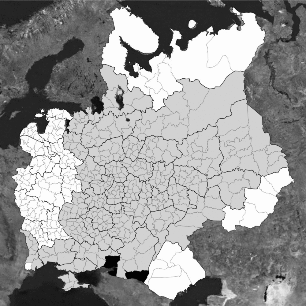
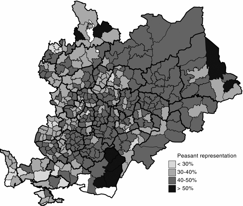
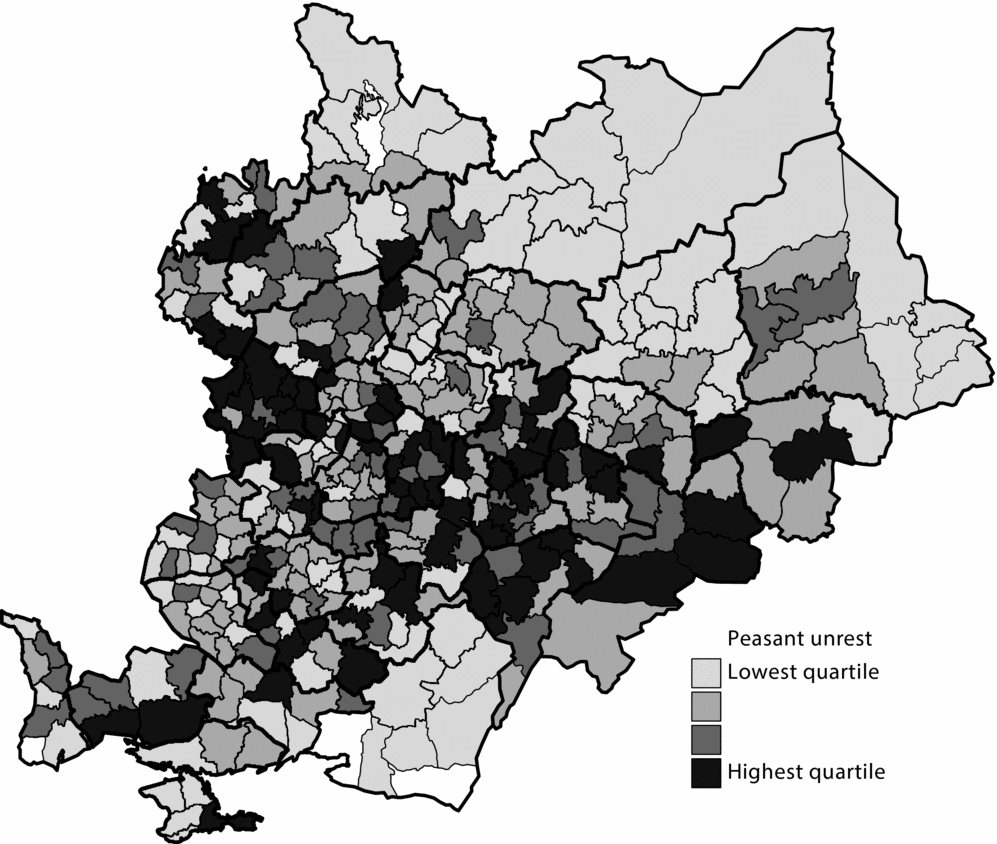
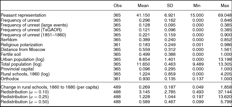
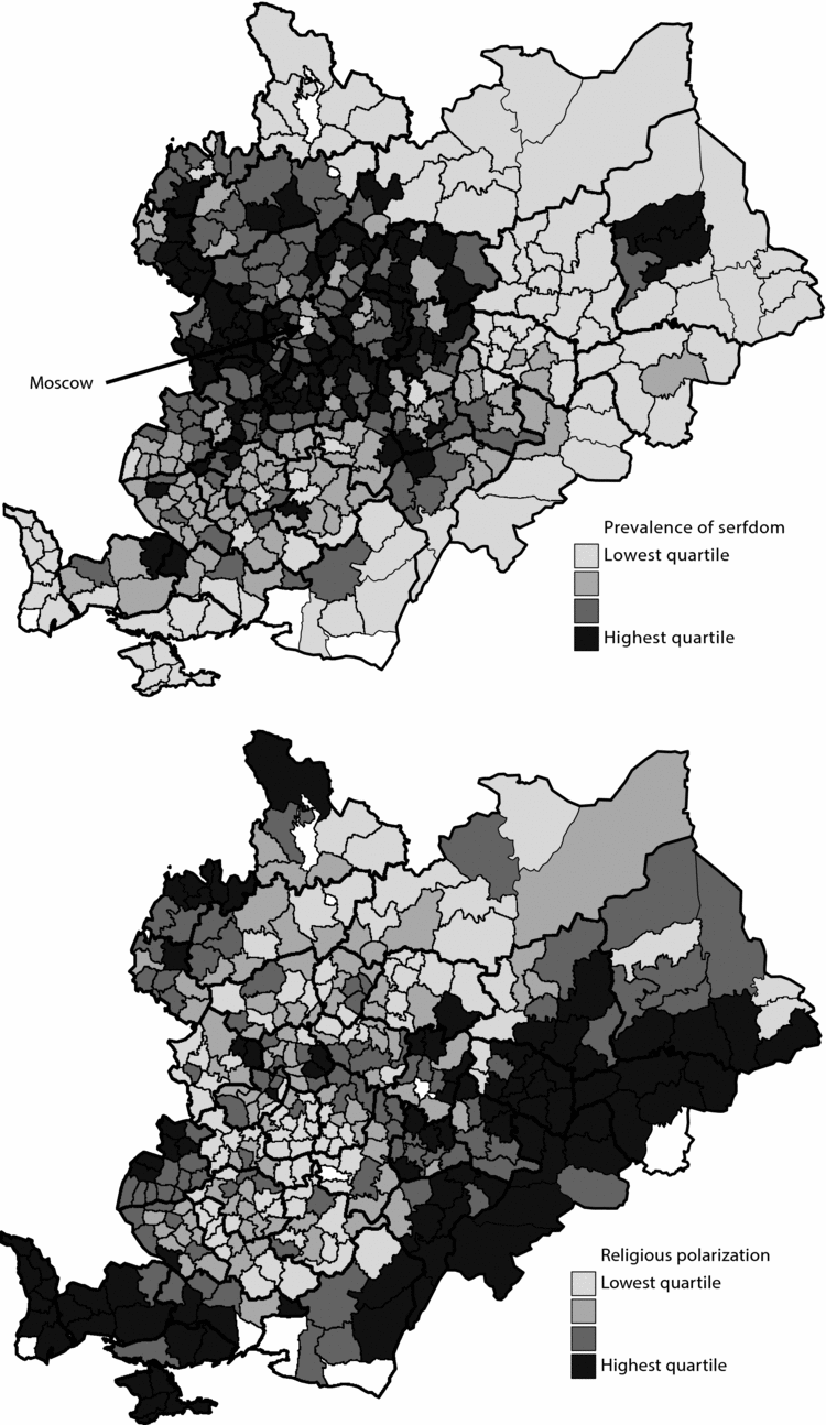
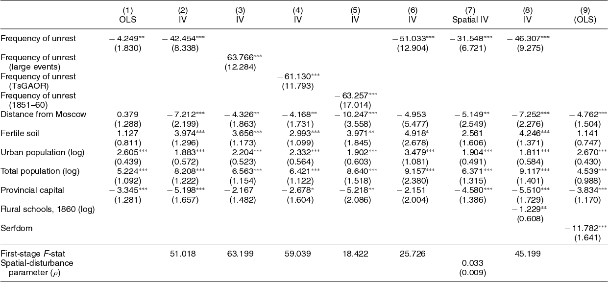
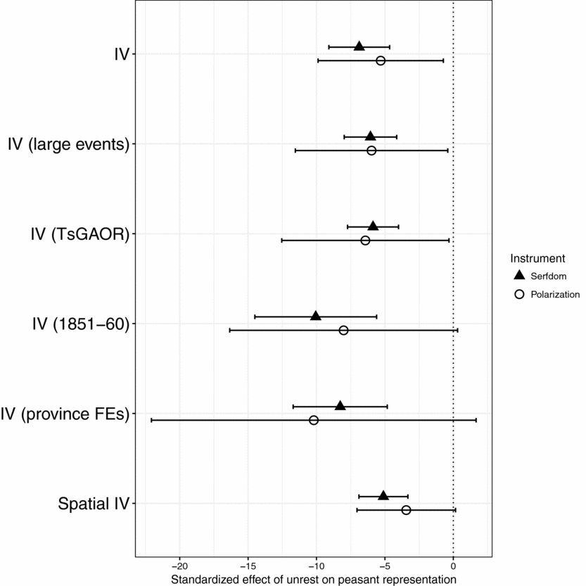
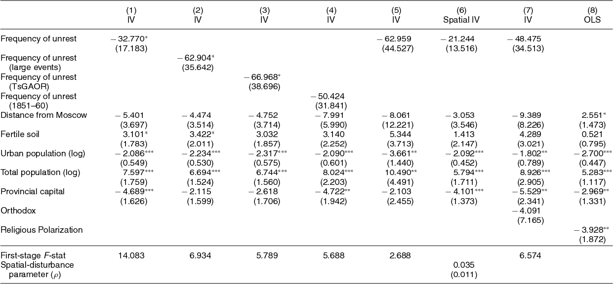
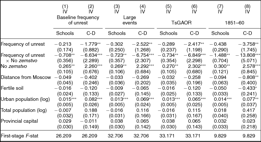




Comments
No Comments have been published for this article.