Introduction
Shape has often been used along with discrete morphologies to investigate many questions in biology and paleobiology, including species discrimination (Budd et al. Reference Budd, Johnson and Potts1994; Villemant et al. Reference Villemant, Simbolotti and Kenis2007; Maderbacher et al. Reference Maderbacher, Bauer, Herler, Postl, Makasa and Sturmbauer2008; Atwood and Sumrall Reference Atwood and Sumrall2012), ontogeny (Rohlf, Reference Rohlf1998; Bookstein et al. Reference Bookstein, Gunz, Mitteroecker, Prossinger, Schaefer and Seidler2003; Sheets et al. Reference Sheets, Kim and Mitchell2004) ecophenotypic variation (Reyment et al. Reference Reyment, Bookstein, McKenzie and Majoran1988; Wilk and Bieler Reference Wilk and Bieler2009; Piras et al. Reference Piras, Marcolini, Raia, Curcio and Kotsakis2010), evolution via heterochrony (Mitteroecker et al. Reference Mitteroecker, Gunz, Weber and Bookstein2004, Reference Mitteroecker, Gunz and Bookstein2005; Lieberman et al. Reference Lieberman, Carlo, de León and Zollikofer2007), functional morphology (Zollikofer and Ponce De Léon 2004), phylogeography (Frost et al. Reference Frost, Marcus, Bookstein, Reddy and Delson2003), and many others (Zelditch et al. Reference Zelditch, Swiderski and Sheets2012). Recent advances involving 3D landmark-based analysis have made marked improvements but nevertheless still rely on an expert handpicking a set of landmark points that represent the geometry of an entire object. The representation of shape by a relatively few landmarks is subjective because user-selected points are chosen for the ease of consistent identification by the user and not necessarily because they represent points with the greatest variance among groups. Additionally, important shape variation outside the landmarks, such as concavity versus convexity, will not be captured by these methods, limiting their usefulness in many situations.
To mitigate these problems, we apply a recent computational-geometry technique called continuous Procrustes distance, or CP distance (see Lipman et al. [Reference Lipman, Al-Aifari and Daubechies2013]). This methodology determines dissimilarity, or distance, between pairs of 3D surface scans of specimens drawn from mixed populations of species. Form taxa are best separated by incorporating a particular combination of geometric features of the 3D scans (such as curvature and area density) into the CP-distance algorithm. The statistical validity of our process is established by contrasting our results with those obtained by Atwood and Sumrall (Reference Atwood and Sumrall2012). More precisely, our benchmarking process shows that the data set contains two clusters and that this classification is equivalent—with a high degree of confidence—to the ones formed by empirically assigned groups of Atwood and Sumrall (Reference Atwood and Sumrall2012).
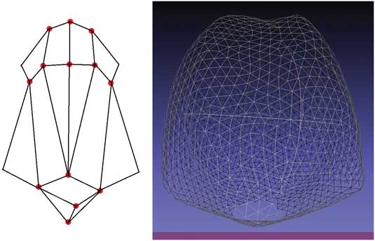
Computational geometry allows us to consider the entire surface 3D scan as data for comparing specimen surfaces, opening the door to incorporating information such as curvature into the analysis. Our results provide strong experimental evidence supporting the use of these techniques for similar studies in different taxa. Our procedure is still time-consuming because of the scanning and mesh-generation phases, which usually take about 1 hour per specimen. This motivated us to explore the effect of lowering scan resolution, which can vastly improve overall speed. To test this concept, we replicate our analysis using artificially produced lower-resolution scenarios. Our proposed methodology is considerably foreshortened because it does not require an expert to choose and record landmarks on the 3D scans. Rather, only a single small hole is made in the mesh at an easily identified homologous point—in this case the circular stem facet at the base of the theca (see Fig. 1 or 2). Our techniques also reduce the potential error resulting from user bias and open the door to incorporating fine-structure, curvature-based features into the analysis.
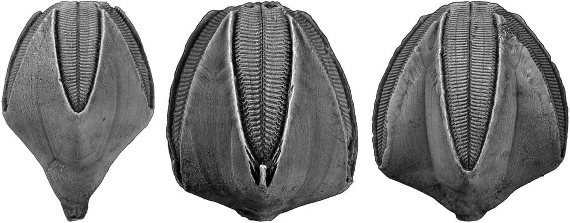
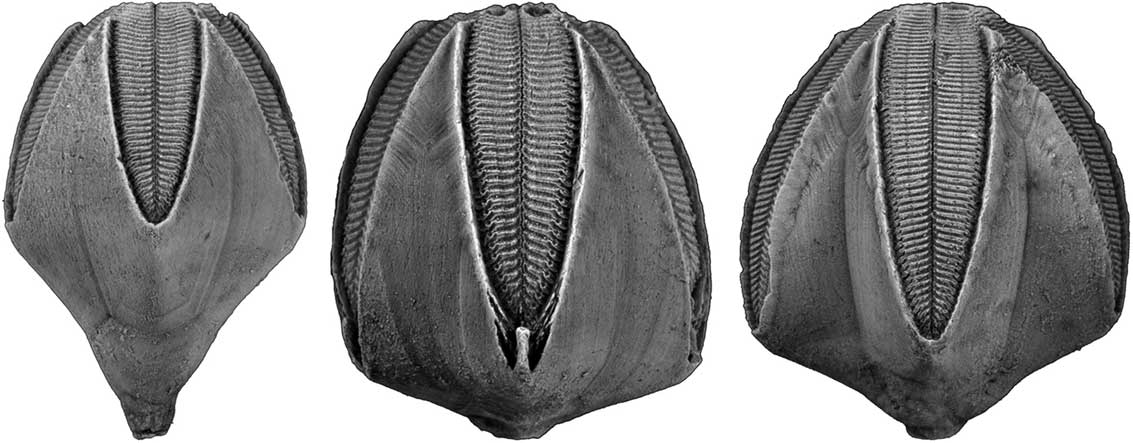
Left, Pentremites pyriformis; middle, P. tulipiformis; right, P. fredericki. P. pyriformis and P. symmetricus are the pyriform samples in this study, while P. tulipiformis, P. fredericki, and P. spicatus are the godoniform samples.
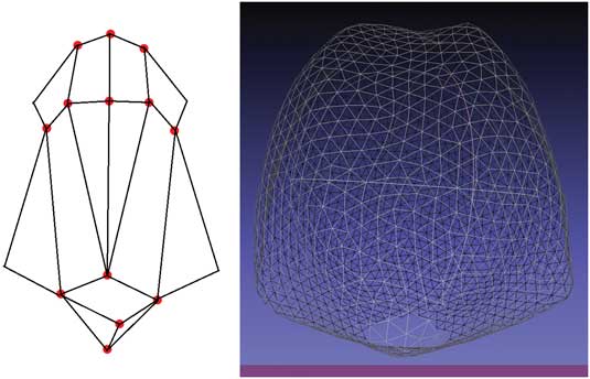
A visual comparison of the data used for computing discrete Procrustes (DP) distance (left image) versus the data used for continuous Procrustes (CP) distance (right image). (See the Approach and Algorithms section for precise definitions.) The images represent samples in the same orientation for clarity of reader comparison, though both methods are unaffected by orientation. Although 13 3D landmark points are chosen (by hand) for computing DP distance (Atwood and Sumrall Reference Atwood and Sumrall2012), the entire 3D scan is used for computing CP distance in this work.
For this study we investigate species discrimination in the Mississippian blastoid echinoderm Pentremites. The bud-shaped theca of blastoids houses the viscera and is commonly well preserved three dimensionally. Much confusion exists concerning species delimitation in Pentremites because: (1) most populations, especially in the Late Mississippian, show high morphological variation; (2) several species cooccur in most localities; and (3) methodology used to describe shape of species lack the power to differentiate specimens into species groups (Waters et al. Reference Waters, Horowitz and Macurda1985; Atwood and Sumrall Reference Atwood and Sumrall2012). Pentremites species can be divided into two morphological groups based on proportions of the theca. The pyriform group includes taxa with an elongated pelvis (the lower part of the theca below the ambulacra) that is similar in size to the vault (the upper part of the theca bearing the ambulacra). The godoniform group includes taxa with a foreshortened pelvis that is much smaller than the vault (Fig. 1). Species delineation within these groups has traditionally relied on the presence of concavities and convexities of ambulacra and interabulacra, vault:pelvis ratios, identification of discrete morphologies, and stratigraphic arguments (Galloway and Kaska Reference Galloway and Kaska1957; Macurda Reference Macurda1975; Waters et al. Reference Waters, Horowitz and Macurda1985; Atwood and Sumrall Reference Atwood and Sumrall2012).
Thecae of the blastoid Pentremites, the main focus of the comparison paper by Atwood and Sumrall (Reference Atwood and Sumrall2012), are ideal for the use of advanced comparison techniques. While three-plate junctions between thecal plates offer obvious type 1 landmarks (Foote Reference Foote1991; Atwood and Sumrall Reference Atwood and Sumrall2012), much of the shape variation in Pentremites occurs in the geometry of the plates themselves; since these lie between landmarks, such details cannot be easily quantified by geometric morphometrics. Moreover, there is great morphological variance within populations of each species, including genetic differences, ecophenotypic variation, and allometry (Macurda Reference Macurda1966; Waters et al. Reference Waters, Horowitz and Macurda1985; Atwood and Sumrall Reference Atwood and Sumrall2012). Although this pilot study focuses on species discrimination, understanding the continuum of shapes for each species using this new technique can ultimately result in more insight on a diversity of issues that will be explored in a forthcoming work.
Materials and Methods
Specimens and Scans
In this study we use two data sets:
-
∙ A set of landmark configurations obtained from Atwood and Sumrall (Reference Atwood and Sumrall2012) via Dryad. These data consist of a set of 13 ordered, handpicked landmark points for each of 52 specimens. The data set is considered as the benchmark group in our study, and we shall use it to validate our algorithm.
-
∙ A new set of 3D scans of 20 Pentremites, chosen to closely resemble those used by Atwood and Sumrall (Reference Atwood and Sumrall2012) to better compare the effectiveness of our proposed methodology. Many of the Atwood and Sumrall (Reference Atwood and Sumrall2012) specimens had to be eliminated a priori because they were incompletely preserved or were heavily encrusted by adhering matrix. This is a limitation of the CP-distance algorithm, which naturally arises when taking the entire surface scan as input data. All specimens were collected from the Upper Mississippian (Chesterian) Glen Dean Formation near Hopkinsville, Kentucky (see Atwood and Sumrall (Reference Atwood and Sumrall2012) for details). All specimens of Pentremites used in this study and in Atwood and Sumrall (Reference Atwood and Sumrall2012) are large, presumably mature individuals chosen to limit allometric effects.
Scans in the new data set were obtained using the Next Engine 3D scanner to capture and preprocess 3D meshes of each blastoid specimen. We used MeshLab to artificially cut out a very small hole in the bottom of each 3D scan, a technical requirement of the CP-distance algorithm. The region removed, the circular stem facet at the base of the theca, was consistent among the specimens and easily identified in the scans. The cutout removes about 0.5% of the points in each scan. This process ensures that the surface has the topological type of a disk; while this is required for the algorithm as is, it is possible to define and compute CP distance for sphere-type surfaces as well.
Approach and Algorithms
Discrete Procrustes distance, or DP distance, is a standard process for comparing a pair of shapes using a predetermined set of landmark points demarked on each surface (i.e., a landmark configuration). This well-known technique gives a quantitative measure of dissimilarity between configurations and was used in Atwood and Sumrall (Reference Atwood and Sumrall2012) to verify the classification of species. Specifically, DP distance finds the minimum value that the sum of all distances between corresponding points within the two landmark sets achieves as the configurations are “aligned” in space (see Atwood and Sumrall [Reference Atwood and Sumrall2012] for details). In contrast, the CP-distance method developed in Lipman et al. (Reference Lipman, Al-Aifari and Daubechies2013) is an extension of the DP distance. It incorporates full geometric information (readily available in 3D scans) such as curvature into the analysis. DP distance is computed via minimizing a sum of distances over a discrete set of landmarks, whereas CP distance is computed via minimizing integrals of geometric quantities. Both methods are scale and rigid-motion invariant. This is to say, the outcomes of the calculations are independent of the size and position/orientation of the scans and resulting landmarks. An overview of the CP-distance algorithm appears in the Supplementary Materials. For specific details, see Lipman et al. (Reference Lipman, Al-Aifari and Daubechies2013).
In this study we use DP distance and CP distance to generate dissimilarity matrices associated to each data set. Each matrix’s i–j entry corresponds to the distance (or dissimilarity) between specimen i and specimen j. These matrices are symmetric, nonnegative, and have only zeros along the diagonal. We first use the DP distance on pairs of landmark configurations from Atwood and Sumrall (Reference Atwood and Sumrall2012) to generate the matrix D At, in an attempt to reproduce the results of Atwood and Sumrall (Reference Atwood and Sumrall2012) in the dissimilarity-matrix language of this study. We then use the CP-distance algorithm on pairs of new 3D scans to generate the dissimilarity matrix D CP. Finally, we devise a methodology for comparing these matrices and determine whether they carry the same “clustering information” within them.
Our specimen scans were performed at the (medium) resolution of 4400 points per square inch. At this resolution, a mesh of about 5000 points represents a typical specimen (Fig. 2). To determine the breaking point of our method, we reran the whole matrix-comparison process using 3D scans artificially downsampled to resolutions of 50%, 20%, 10%, and 5% of the original scans. Downsampling was carried out using quadric edge collapse in MeshLab.
In this work we deploy three methods for comparing dissimilarity matrices and their cluster information:
-
1. Mantel’s test (performed on two dissimilarity matrices of equal size) is used to check for correlations between each distance’s interspecimen measurements.
-
2. A multidimensional scaling algorithm is used for visualizing cluster information.
-
3. Aggregate clustering is applied to understand groupings at different scales.
1. Mantel’s Test Methodology
Mantel’s test is a standard statistical tool used to compare distance matrices, often used in a biological setting with actual distances (Sokal and Rohlf, Reference Sokal and Rohlf2012). Here we use Mantel’s test to compare the distance matrices D CP and D At. It is important to note that both matrices represent mathematical metrics on the same kinds of objects, making this comparison a classical and direct use of Mantel’s test. The dimensions of these matrices must be equal for Mantel’s test to be used. Because we were not able to obtain full 3D scans of all the specimens of the Atwood and Sumrall (Reference Atwood and Sumrall2012) study, the dissimilarity matrices D At and D CP are of different sizes. To overcome this and at the same time use the most information possible, we proceed as follows. We randomly choose 20 specimens from within Atwood’s landmark data (52 specimens total) and produce a “submatrix” of D At corresponding to the intersample DP distances between these 20 specimens; moreover, we make sure that the number of specimens from each species matches the amount in D CP. This sampling method means that the results of our test will address how similar the metrics are when considering the comparison of different species. We then carry out Mantel’s test between D CP and the randomly sampled submatrix of D At. The sampling process is repeated 5000 times, 1000 times for each one of the four possible resolutions: 100%, 50%, 20%, and 10%, and once to cross-compare D At with itself to see the effect of the sampling method on correlation values.
In addition, Mantel’s test was also performed pairwise between different resolutions of D CP. This process was repeated 10,000 times, 1000 times for each possible pairing. We note that at 5% resolution, three of the samples could not be processed by the CP distance due to lack of mesh points. (We observed a threshold of about 80 mesh points for the algorithm to work.) Because of this, our Mantel’s test with 5% resolution always involves sampling of P. tulipiformis.
2. Multidimensional Scaling (MDS) Algorithm
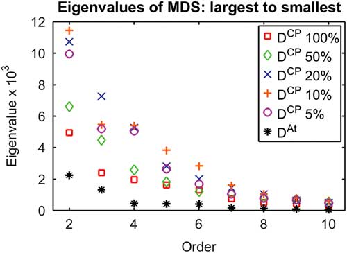
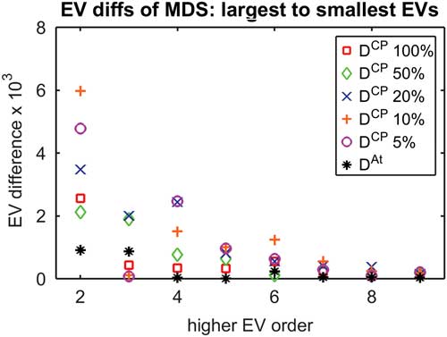
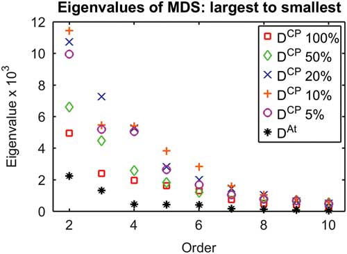
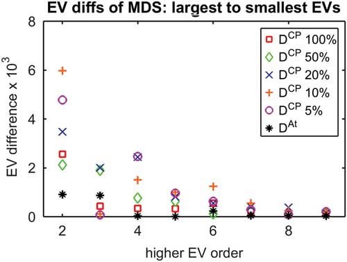
MDS is a tool used for dimensional reduction or presentation of complicated high-dimensional data (Cox and Cox Reference Cox and Cox2001). We use this procedure to obtain a “visual realization” of the cluster structures that lie within the dissimilarity matrices. The MDS methodology differs little from the principal components analysis method (PCA) used in Atwood and Sumrall (Reference Atwood and Sumrall2012) but presents some graphical advantages. For example, it allows us to remove the requirement of a global landmark alignment. For our aggregate clustering, MDS was used with six dimensions. This number is chosen based on a drop in the eigenvalues of the resulting covariance matrix, in a manner similar to what is done for PCA (Fig. 3). The dimension is fixed on all runs to obtain consistency across the clustering procedure.
Diagram depicting the second through tenth eigenvalues of the MDS procedure for each dissimilarity matrix. For most matrices, there is a noticeable decline between eigenvalues 6 and 7, and so six eigenvalues were used for all clustering algorithms at all resolutions for consistency. The first eigenvalue is always much larger than the rest, and so is omitted for scale purposes.
3. Aggregate Clustering (AC)
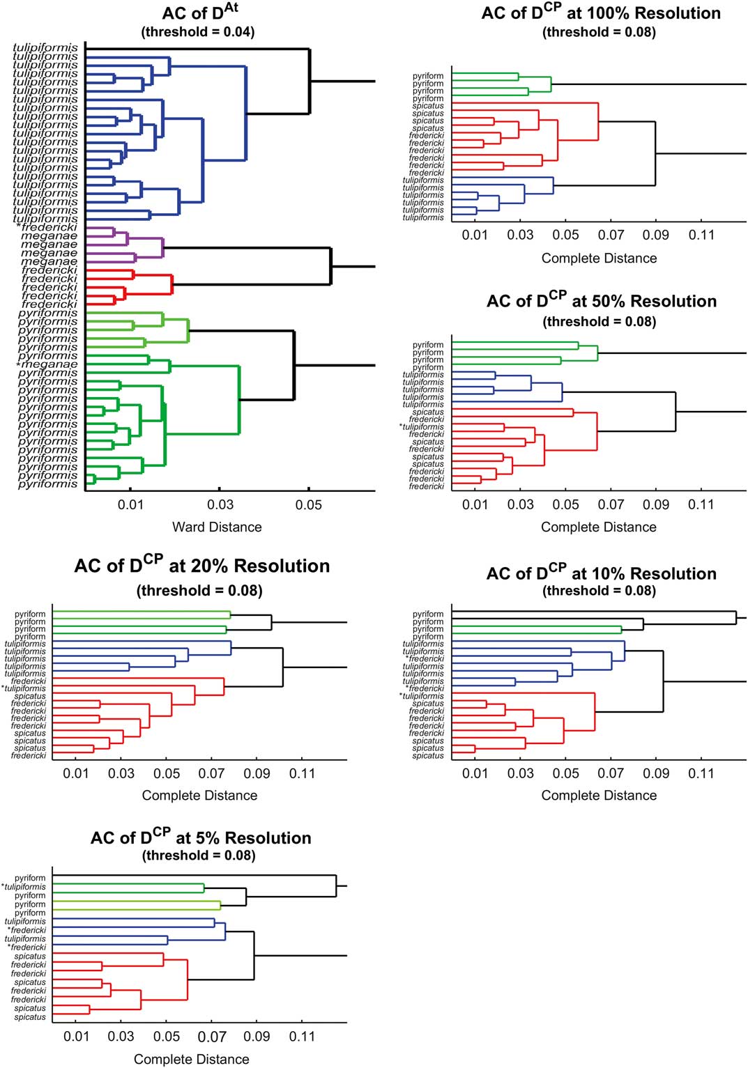
AC is a well-established method (Tan et al. Reference Tan, Steinbach and Kumar2005). It is particularly useful for determining clusters within data sets. It produces dendrograms, which convey grouping information at different scales (Fig. 6). Within AC, we use the complete algorithm for all resolutions of D CP, because it is appropriate for high-dimensional data sets but does not assume our clusters have any particular shape (Ferreira and Hitchcock Reference Ferreira and Hitchcock2009). The Ward algorithm was used for D At, because it is the best general agglomerative method, we expect elliptical clusters from our MDS graph (Ferreira and Hitchcock Reference Ferreira and Hitchcock2009), and the Ward algorithm yields results most similar to those in Atwood and Sumrall (Reference Atwood and Sumrall2012).
To test for robustness, we performed a cross-validation. The Ward AC was repeated on random samples of 90% of the (D CP or D At) specimens. The resulting clustering is given labels and used to classify the remaining 10% by the cluster of each specimen’s nearest neighbor. This classification is then compared with the results of Atwood and Sumrall (Reference Atwood and Sumrall2012) for benchmarking purposes; we aim to reproduce the number of correct identifications. For this process, the data was always split into three clusters, with labels of (1) P. fredericki/P. spicatus, (2) P. tulipiformis, and (3) P. pyriformis. The same labels are used to describe the benchmark group, although P. spicatus is not present in these data.
Results
For each level of resolution, we performed Mantel’s test with 1000 iterations over 1000 random samples of submatrices of D At. Our results (Table 1, left) show that the correlation between the submatrices of D At and D CP is consistently above 70%, with a very low p-value (p-value<10-6) at all levels of resolution. Considering all possible multiple-way comparisons, we can express an overall p-value of at most 0.00072.
Left, average correlations between D At and different resolutions of D CP via Mantel’s test. These simulations all involve the same sampling scheme, so they can be directly compared. Right, table of average correlations between different resolutions of D CP via Mantel’s test. No sampling occurs except in the rightmost column.

Mantel’s test was also performed between different resolutions of CP distance. Our results (Table 1, right) show correlation between 100% and 50% resolution is above 97%. Similarly, 10% and 5% resolution are highly correlated. The correlations between higher and lower resolutions are lower, suggesting a qualitative change as resolution drops.
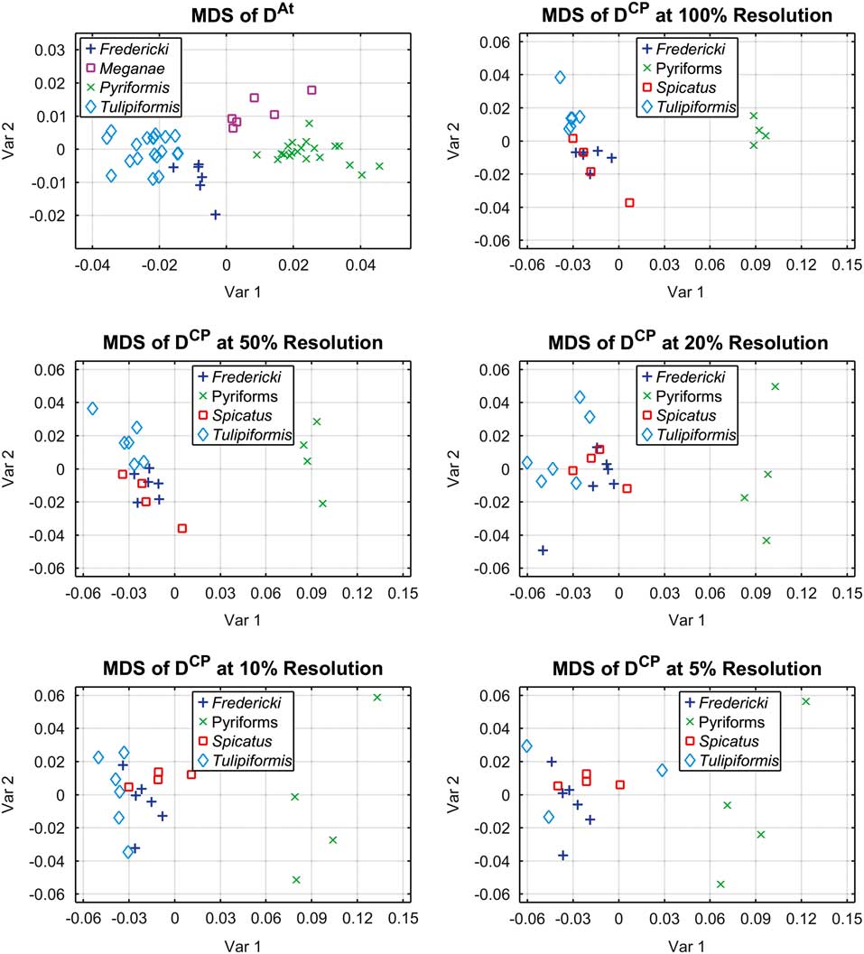
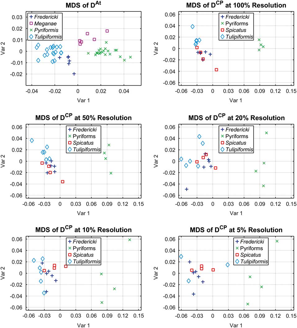
The next step in the comparison process was to implement the MDS algorithm on the dissimilarity matrices D CP and D At at all five resolutions. (Note that this method does not require the matrices to be of equal size.) The output of this algorithm consists of the plots displayed in Figure 4. An interesting observation is that the variance observed in the plot within each species’ cluster increases as the resolution decreases. Careful attention to individual specimens also reveals that the horizontal component in the plot captures how elongated specimens are and thus divides the pyriform and godoniform groups quite naturally. On the other hand, it appears that the vertical component in the plot captures the concavity between ambulacra. However, since the MDS algorithm does not embed the data set directly onto coordinate axes (as does the alternative method, PCA), these interpretations are rather hard to prove.
Each plot conveys a particular MDS, where individual titles indicate which dissimilarity matrix was used as input. Similar to PCA, Var 1 represents the direction with highest variance and Var 2 represents the direction with second-highest variance.
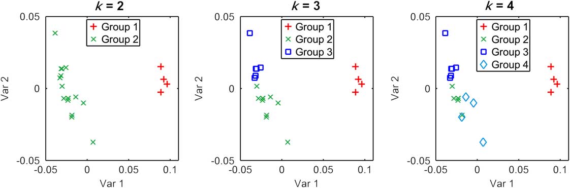
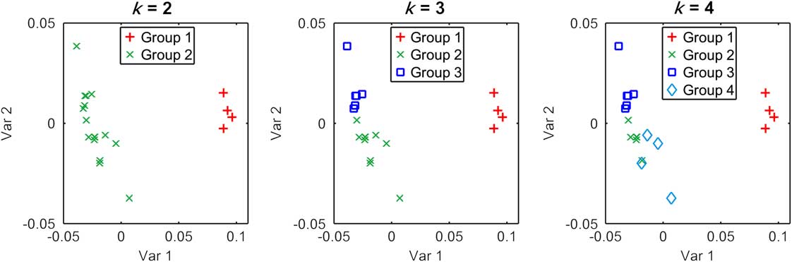
The final step in the analysis consists of deploying AC on the dissimilarity matrices D CP and D At at all five resolutions. Like MDS, this method also does not require the matrices to be of equal size. Dendrograms of these clusters can be seen (Fig. 6). We can also see the progression of variance as clusters are aggregated (Fig. 7). This progression of variance helps us to determine that there are three clusters present in our data. Figure 5, which depicts k-means as performed on our MDS embedding, also supports our clustering choice. k-means with k=3 splits our data into the same three groups as the AC does.
k-means was performed with the MDS embedding of 100% resolution D CP, resulting in the figures shown. Left, k=2; center, k=3; right, k=4. These divisions help support the results of our aggregate clustering.
A visual analysis of the AC outcome of Figure 6 shows that the CP-distance dissimilarity matrix manages to clearly separate P. tulipiformis from the cluster containing P. fredericki and P. spicatus samples. This improves the result of the comparison study by Atwood and Sumrall (Reference Atwood and Sumrall2012), in which the separation of P. tulipiformis and P. fredericki is incomplete, and a few P. fredericki samples are (incorrectly) categorized as P. tulipiformis. Furthermore, while both old and new methods separate P. pyriformis from the other species, CP distance–based analysis does a better job. Indeed, it separates the data into two distinct, large clusters that correspond to the pyriform and godoniform groups; moreover, it is evident that this clustering happens at a coarser level than the separation of species. Finally, we see that as the resolution of scans decreases, the advantages of CP-distance method over the traditional techniques disappear: at 20% resolution, CP distance no longer separates P. tulipiformis and P. fredericki better than DP distance. However, even at 5% resolution, the larger clusters of the pyriform and godoniform groups still clearly separate, and some (coarse) information still can be obtained.
Each dendrogram depicts hierarchical AC on a different dissimilarity matrix. All D CP matrices used complete distance due to small sample numbers (so cluster shape is unclear), while D At used the ward algorithm to compute distance between clusters. Distance thresholds were chosen so that the resulting clusters are preserved under larger perturbations. Errors in classification are marked with an asterisk. One primary shortcoming can be seen readily in these dendrograms: P. spicatus and P. fredericki are not well separated.
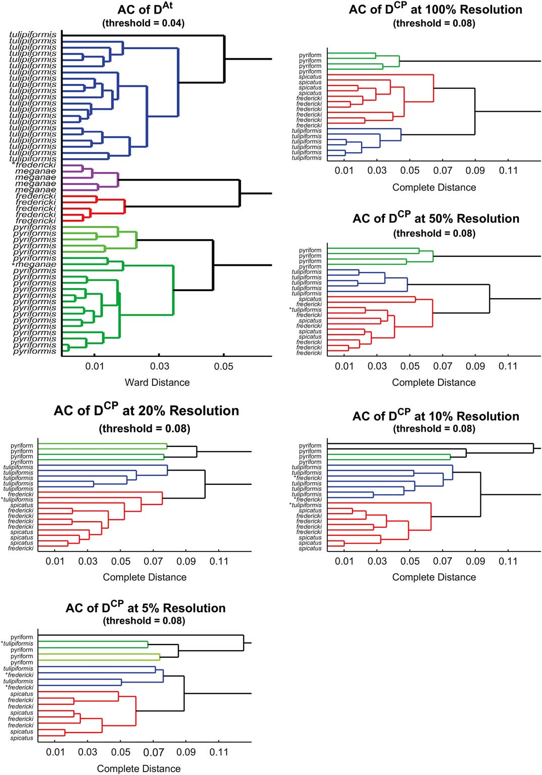
Figure 7 depicts the results of our cross-validation procedure. For each trial, Ward AC was used to cluster 90% of our data. These clusters were used to classify the remaining 10%, and these were compared to the benchmark group. The details of the procedure can be seen in Table 2.
Depiction of the amount of variance needed to agglomerate each cluster (as indicated in the horizontal axis) for each data set. EV, eigenvalues (of the variance matrix). We can consider this as the variance accounted for by each particular transition (e.g., from two to three clusters). The first datum is absent because it is much larger than the rest. After the transition from two to three clusters, the rest account for about the same amount of variance, so we conclude that there should be three clusters.
Reliability of our method’s ability to cluster and ultimately classify species of Pentremites. Left, each column depicts the results of our cross-validation for a particular resolution of data using D CP. Ninety percent of our data was sampled, and there are only two remaining specimens to be classified. The percentage of trials with each number of correct classifications is listed. The bottom row depicts the overall proportion of classifications that were correct. Right, analogous table using D At on five remaining samples (10% of the total), no variation in resolution. Each cross-validation experiment was done with 10,000 sampling trials.

Discussion
One of the most evident advantages of the CP distance–based methodology over the DP-distance procedure is the speed at which samples can be analyzed. Although both analyses require specimens to be scanned, the proposed methodology nearly eliminates the tedious (and human error–prone) landmark-picking phase. An evident advantage of the traditional method in the blastoids example is that it can be deployed using only a portion of the surface scan, because the full set of landmarks lies entirely on one side of the specimens due to strong (pentagonal) symmetry; an extension of this work consists in taking specimen symmetry into consideration when applying our framework. Nevertheless, this gain does not translate into an overall advantage in speed, as landmarks have to be marked under a microscope a priori, so that they can be identified, and their position recorded a posteriori, because their position can be documented visually but is not evident in the scans (Atwood and Sumrall Reference Atwood and Sumrall2012). Consequently, the identification of landmarks on the thecal surface requires knowledge of blastoid morphology to orient the specimens and identify the particular three plate junctions that serve as landmarks and manual dexterity to mark the landmarks properly. The process provides two points for user error to enter into the analysis—the initial marking of the landmarks and the recording of their position on the scans. In contrast, our CP distance–based method only requires marking the position of the stem facet, which is easily seen on the scans. Therefore, our method nearly eliminates sources of human error because its continuous description of shape is independent of how the observer records the data.
The proposed CP-distance methodology also provides advantages when compared with traditional methods by taking into consideration a more complete representation of specimen morphology. This is achieved by incorporating fine-scale shape measurements such as curvature. Indeed, a natural progression is seen when going from the vault:pelvis and height:width ratios to summarize shape (encoded as a 2D rectangle) to the DP-distance landmark analysis based on 3D scans, in which 13 points represent the specimen’s shape. In this context, our methodology now uses the full geometric information of each specimen’s shape. Advances in computer imagery allow us to deploy this sophisticated technique on very-high-resolution scans, which represent an object’s shape accurately with thousands or even tens of thousands of points.
CP distance–based analysis could potentially have a tremendous impact in the study of organisms that have a distinct shape but lack homologous landmarks, which makes morphometric analyses impossible. Such studies may include growth of colonial organisms or investigating ecophenotypic variation in organisms such as corals, sponges, and stromatolites.
Traditional landmark analysis has advantages in two areas over CP-analysis. First, type 1 landmarks, as used in the Atwood et al. (2012) study, are points that have anatomical homology between specimens. Whereas calculated geometric “feature points” may change position between species, the type 1 landmarks represent identical points, allowing for different types of questions to be addressed; however, as mentioned above, landmarks could be used as the feature points for CP distance in a future study.
Second, landmarks used for the Atwood et al. (2012) study require preservation of only the A ambulacrum and adjacent interambulacra for any given specimen. Specimens could be analyzed with confidence even if other portions of the theca were missing or covered with matrix. The CP-distance method, as presently used, requires complete preservation of thecal surfaces preserved three dimensionally and without significant adhering matrix. Our forthcoming work will address both of these issues.
Conclusion
We compare a novel computational-geometry methodology based on continuous Procrustes distance with the standard method of discrete Procrustes distance for tackling the problem of species discrimination on Pentremites. Our results show that the CP-distance methodology is not only (slightly) superior at resolving the issue but also significantly reduces processing time and vulnerability to human error.
Specifically, advantages appear in the separation of P. tulipiformis species from the cluster containing the P. fredericki and P. spicatus species. In contrast, Atwood and Sumrall (Reference Atwood and Sumrall2012) clusters a few P. fredericki as P. tulipiformis, and the respective clusters are visually mixed. We attribute this advantage to the CP-distance calculation taking into consideration curvature measurements, which reflect the concavity of the specimens’ plates. This differs significantly from the output that can be obtained using DP distance alone; in that methodology, concavity is measured only as a subtle change in the position of a couple of landmarks. This phenomenon is vastly amplified when large regions of the sample are concave and eventually adds up to a large difference in the resulting CP distance. As a consequence, we are effectively able to separate species that are concave from those that are not.
In addition, we determined the sensitivity of the CP-distance methodology to varying resolutions of scans. We found a threshold of approximately 1000 points per scan, under which the reliability of the method begins to wither. Nevertheless, we showed that even at the lowest resolution levels there is information to be gained. Because of the relatively low cost and short time involved in performing low-resolution scans, our technique opens the door for future researchers in the area to produce several low-cost, preliminary studies; this would allow them to choose where to invest their in-depth efforts more effectively.
Acknowledgments
The authors would like to thank two anonymous reviewers for their comments, which substantially improved the manuscript. Special thanks to J. A. Waters at the Appalachian State University for very helpful conversations and B. Allen at the University of Tennessee, Knoxville, for suggestions and discussions.
Supplementary Material
Data available from the Dryad Digital Repository: http://dx.doi.org/10.5061/dryad.cg7b7