1 Introduction
The study of vortex rings has a long history, extending back to the 19th century (for example, von Helmholtz Reference von Helmholtz1858). Since that time, the study of vortex rings has been integrated into nearly every domain of fluid dynamics (see Shariff & Leonard Reference Shariff and Leonard1992, and the examples therein). This paper investigates the three-dimensional mechanics of vortex rings interacting with a stratified interface. For clarity, the complete dynamics that results from the interaction of the vortex ring with a density stratification will be simply denoted as the ‘vortex-ring interaction’ in what follows.
At the start of the 20th century, there was uncertainty whether vortex rings were stable fluid structures. Crow (Reference Crow1970) demonstrated that a vortex dipole of constant vorticity was unstable to coupled long-wavelength perturbations. Widnall & Sullivan (Reference Widnall and Sullivan1973) applied Crow’s argument to the case of a vortex ring with a large radius of curvature, demonstrating that (nearly) all vortex rings with a finite core size are unstable. However, the wavelength of the experimentally observed perturbations was short with respect to the core diameter, in violation of the long-wavelength analysis. Subsequent analysis (see Widnall, Bliss & Tsai Reference Widnall, Bliss and Tsai1974; Moore & Saffman Reference Moore and Saffman1975; Widnall & Tsai Reference Widnall and Tsai1977; Tsai & Widnall Reference Tsai and Widnall2006) has shown that the fastest growing instability for both a dipole and the vortex ring is an example of an elliptic instability. Bayly (Reference Bayly1986) and Pierrehumbert (Reference Pierrehumbert1986) demonstrated this instability in a broad class of straining flows; see Kerswell (Reference Kerswell2002) for a review of elliptic instabilities. Experimentally, the instability of vortex rings has been observed by Krutzsch et al. (Reference Krutzsch, Bolster, Hershberger and Donnelly1939) and more recently by Maxworthy (Reference Maxworthy1977). A recent publication (Ponitz, Sastuba & Brücker Reference Ponitz, Sastuba and Brücker2015) has presented a full three-dimensional experimental visualization of the elliptic vortex-ring instability observed in an unstratified environment, and compares well with the numerical work of Archer, Thomas & Coleman (Reference Archer, Thomas and Coleman2008). In this paper, we investigate vortex rings that are modified in the presence of a stratification.
The impact of vortex rings on a solid wall has also been studied in the literature (Orlandi & Verzicco Reference Orlandi and Verzicco1993; Swearingen, Crouch & Handler Reference Swearingen, Crouch and Handler1995; Munro, Bethke & Dalziel Reference Munro, Bethke and Dalziel2009). The vortex ring expands as it approaches the wall, and, due to the no-slip boundary condition, secondary vorticity is produced. The interaction of the primary vortex ring with the secondary vorticity results in an instability on the secondary vorticity surface. Both Orlandi & Verzicco (Reference Orlandi and Verzicco1993) and Swearingen et al. (Reference Swearingen, Crouch and Handler1995) interpreted this instability as a result of the straining field produced by the primary vortex ring. More recently, Harris & Williamson (Reference Harris and Williamson2012) investigated the impact of a vortex dipole on a solid wall and argued that the resultant instability in the secondary vorticity field is primarily due to a Crow instability but is often misinterpreted as an elliptic instability due to the similarity in the instability wavenumber. We will see that this earlier work has direct applicability to the case of a vortex ring impacting a stratified interface. For a vortex ring impacting a free-slip surface, there is no secondary production of vorticity, and thus the vortex ring continues to expand in the presence of its image ring (using the method of images). As demonstrated by Archer, Thomas & Coleman (Reference Archer, Thomas and Coleman2009), the interaction of the vortex ring with its image will result in an elliptical instability followed by a Crow instability.
While topologically distinct, an understanding of the dynamics of dipoles has played a key role in understanding the dynamics of vortex rings, and vice versa. See Leweke, Dizs & Williamson (Reference Leweke, Dizs and Williamson2016) for a review of the dipole instabilities. The work of both Nomura et al. (Reference Nomura, Tsutsui, Mahoney and Rottman2006) and Ortiz, Donnadieu & Chomaz (Reference Ortiz, Donnadieu and Chomaz2015) highlights the role of stratification on the instability of vortex dipoles. In both of these studies, the stratification was chosen to be linear and the Richardson number (defined below) was restricted to be no greater than unity. As the dipoles propagate, stratification is observed to significantly enhance the instability as the two vortices are pushed together, resulting in an enhanced straining field, and hence a rapid growth of an elliptic instability. For a Richardson number much less than one, the instability grows in essentially the same manner as the unstratified case. For a Richardson number equal to one, Ortiz et al. (Reference Ortiz, Donnadieu and Chomaz2015) used a linear adjoint-loop optimization technique and showed that the wavenumber of maximum growth occurred for an antisymmetric perturbation (identified as an elliptic instability) with a growth rate greater than twice the unstratified case.
Similarly, the evolution of vortex rings is modified in a stratified environment (see Turner Reference Turner1957; Atta & Hopfinger Reference Atta and Hopfinger1989; Scase & Dalziel Reference Scase and Dalziel2006). To the best of our knowledge, no analytic theory currently exists that has explicitly investigated the linear stability of vertically propagating vortex rings in a stably stratified environment. Early work on the interaction between a vortex ring and a two-layer stratification is found in the paper by Linden (Reference Linden1973), who investigated the bulk mixing of the density field as a result of the vortex-ring breakdown. The work of Dahm, Scheil & Tryggvason (Reference Dahm, Scheil and Tryggvason1989) presents two-dimensional images of a dyed vortex ring impacting upon a sharply stratified interface. Numerical investigation of vortex-ring interactions with a stratification has become increasingly popular in recent years due to the increase in computational resources available. Stock, Dahm & Tryggvason (Reference Stock, Dahm and Tryggvason2008) numerically simulated the inviscid vortex-ring interaction and observed relatively small-amplitude three-dimensionalization, although they did not characterize the instability. Camassa et al. (Reference Camassa, Khatri, Mclaughlin, Mertens, Nenon, Smith and Viotti2013) also investigated (using both experimental and numerical techniques) the interaction of dense vortex rings with an interface and observed a parameter space division between trapped and escaping vortex rings.
This paper presents an experimental investigation of the stability of vortex rings in a stratified environment. An understanding of the mechanics of this interaction will help to quantify why vortex rings have been observed to be such efficient mixers (Olsthoorn & Dalziel Reference Olsthoorn and Dalziel2015). We begin with an analysis of the two-dimensional dynamics of the vortex rings as they impact a density interface. In order to analyse the three-dimensional dynamics, we reconstruct the full three-dimensional velocity field of a vortex ring vertically impacting onto a stratified interface. We achieve this reconstruction through the use of a stereo-PIV (stereoscopic particle image velocimetry) set-up, which determines the three components of velocity on a single horizontal plane. By moving the height of this horizontal light sheet relative to the density interface, we determine the three components of velocity for a range of level heights. By combining these results, we reconstruct a three-dimensional image of the interaction of the vortex ring with the density stratification. The limitations of this methodology, including a verification of its validity, will be discussed below. Experimental and theoretical evidence suggests strong qualitative and quantitative agreement between the reconstructed velocity field and the true interaction.
The remainder of this paper is organized as follows. Section 2 provides two-dimensional simultaneous PIV/laser-induced fluorescence (LIF) measurements of a vortex-ring interaction with a stratified interface for a range of Reynolds and Richardson numbers. Section 3 details the experimental set-up, image capture and processing methodology for the three-dimensional visualization, followed by § 4, which presents a detailed analysis of the evolution of the velocity field. Finally, Section 5 concludes and suggests possible extensions of the present work.
2 Vertical-slice observations
In a water-filled tank (
 $0.20\times 0.40\times 0.50~\text{m}^{3}$
), we produced vortex rings, which propagated vertically downwards towards the base of the tank. Vortex rings were generated by driving a computer-controlled linearly actuated bicycle pump (0.029 m internal diameter), which was connected to a partially submerged hollow cylindrical tube (internal diameter
 $D=0.039~\text{m}$
). The vortex tube was inserted to an approximate depth of 0.13 m. This set-up is similar to that found in Olsthoorn & Dalziel (Reference Olsthoorn and Dalziel2015). In both the vertical-slice measurements found here and the horizontal-slice measurements found below, the base of the vortex tube was always positioned at least two vortex diameters away from the density interface. This criterion ensured that the density interface did not affect the formation of the vortex ring.
A vertical light sheet was produced within the tank, oriented so that each vortex-ring axis was coplanar with the laser sheet. This laser sheet was generated by a frequency-doubled double-pulsed neodymium–YAG (Nd:YAG) laser (Litron Lasers). Each 532 nm beam was fired at a rate of 99 Hz. Two cameras (Teledyne DALSA, Falcon2 4M180) equipped with 60 mm (
 $f/2.8$
) Nikon lenses were positioned facing the tank. The fluid within the tank was seeded with
 $20~\unicode[STIX]{x03BC}\text{m}$
polyamide particles (
 $\unicode[STIX]{x1D70C}_{p}\sim 1.02~\text{g}~\text{ml}^{-1}$
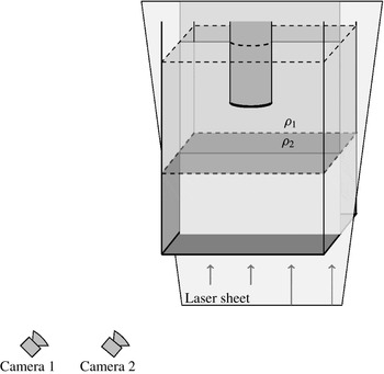
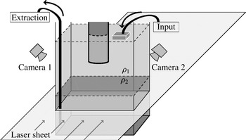
), which had a settling velocity of the order of 0.005 % of the vortex-ring propagation speed. The cameras recorded the motion of the particles within the light sheet at 99 frames per second. Both the laser and cameras were triggered via the connected computer system, allowing for precise laser-pulse/camera-frame triggering and synchronization. The methodology to compute the velocity field is similar to that found in Bethke & Dalziel (Reference Bethke and Dalziel2012). Figure 1 presents a diagram of the experimental vertical laser-sheet set-up. Two cameras were positioned facing the front of the tank and the laser sheet was positioned such that it bisected the vortex tube. The two cameras were oriented such that their plane of focus was coplanar with the laser sheet. A florescent dye was added to the lower layer. We return to this later.
Diagram of the tank set-up for a vertical laser sheet. It should be noted that the laser sheet is positioned such that it bisects the vortex tube.

For both of the vertical-slice results presented here, and the three-dimensional results presented later, we initialized the experimental tank with a two-layer stratification. The stratification was generated using a peristaltic pump to slowly inject the denser fluid (
 $\unicode[STIX]{x1D70C}_{2}$
) beneath a layer of less dense fluid (
 $\unicode[STIX]{x1D70C}_{1}$
). This methodology has been previously shown to produce sharp interfaces (Olsthoorn & Dalziel Reference Olsthoorn and Dalziel2015). Typically, these two fluid layers would have different refractive indices, which would distort the camera images. Due to the small size of the PIV particles, even small variations in the refractive indices of the two layers would defocus the particles, which would corrupt PIV computation. With the careful balance of sodium chloride (NaCl) and sodium nitrate (
 $\text{NaNO}_{3}$
) in the upper and lower fluid layers respectively, we were able to match the refractive indices of the two-layer system. Sodium nitrate is an ideal choice for a secondary salt as it is low cost, relatively safe, allows for index matching over a relatively large density range and is easily disposable. There is minimal difference between the diffusivities of sodium chloride and sodium nitrate in solution (see below), and the mixing of solutions was near linear at the concentrations used here. In principle, the refractive index of each layer will depend on its respective salt concentration, in addition to the temperature of the two layers and the wavelength of the incident light. In practice, for a near uniform temperature profile within the tank and single wavelength light source, these additional dependencies were negligible in the experiments presented here. This salt-solution methodology is similar to that employed by McDougall (Reference Mcdougall1979) for studying plumes. For the vertical-slice experiments performed, we additionally added a small concentration of rhodamine 6G to the denser fluid (
 $\unicode[STIX]{x1D70C}_{2}$
, sodium nitrate layer), which was fluorescent when illuminated by the 532 nm laser. A 575 nm low-pass filter was then added to one of the DALSA cameras to filter out any light from the PIV particles within the tank. The other DALSA camera was fitted with a 3 nm wide notch filter so that only the particles were visible.
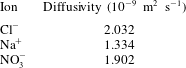
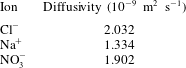
We briefly make note of the cross-diffusivities of the two different salt solutions. The diffusion rate of either salt should not be substantially different due to their similar molecular mass. For reference, the diffusion rate of each ion present in solution is found in the Handbook of Chemistry and Physics (Haynes Reference Haynes2012) and presented in table 1. It should be noted that the difference in the coefficient of diffusivity of each ion is within a factor of two. In order to maintain a charge balance within the stratification, ions of different charge must remain paired. Hence, we note that, as the difference between the ionic diffusivities of chlorine and nitrate is an order of magnitude lower than either constituent, we are confident that double diffusion will not play a role. We note that the maximum duration of the refractive-index-matched experiments was very fast (approximately 6 h) compared with the diffusion time scale of the system. We did not pursue this further in this paper.
Table of the diffusivities of the various ionic species found in our experiments. Diffusivities can be found in Haynes (Reference Haynes2012).
Three two-layer stratifications were produced with different top-to-bottom density jumps
 $\unicode[STIX]{x0394}\unicode[STIX]{x1D70C}$
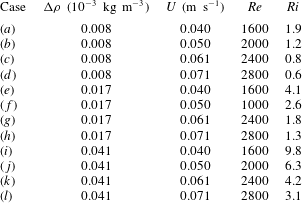
. The refractive index of the stratification was matched in all cases. For each density stratification, vortex rings with four different parameter sets were generated within the tank. This set of 12 cases allowed us to evaluate the vortex-ring interaction for a suite of parameter values. Table 2 presents these 12 parameter cases along with their corresponding Reynolds (
 $Re$
) and Richardson (
 $Ri$
) numbers, defined as
 $$\begin{eqnarray}Re=\frac{DU}{\unicode[STIX]{x1D708}},\quad Ri=\frac{g\unicode[STIX]{x0394}\unicode[STIX]{x1D70C}}{\unicode[STIX]{x1D70C}_{0}}\frac{D}{U^{2}}.\end{eqnarray}$$
Here,
 $U$
is the propagation speed of the vortex ring,
 $g$
is the acceleration due to gravity,
 $\unicode[STIX]{x1D708}$
is the molecular viscosity of the fluid and
 $\unicode[STIX]{x1D70C}_{0}$
is a reference density, here taken to be
 $\unicode[STIX]{x1D70C}_{0}=1\times 10^{3}~\text{kg}~\text{m}^{-3}$
. The length scale was selected to be the diameter of the vortex tube,
 $D$
. An alternative length scale would be the vortex-ring diameter (
 $a$
); however, Maxworthy (Reference Maxworthy1977) demonstrated a weak parameter dependence on the ratio
 $a/D$
. Due to the difficulty of perfectly aligning the light sheet with the propagation axis of the vortex rings, and thus a precise determination of
 $a$
, we selected the length scale to be that of the tube diameter, but noted the ratio
 $a/D\approx 1.25$
(shown below), as observed previously by Maxworthy (Reference Maxworthy1977).
Table of the parameter values associated with the 12 vertical-slice vortex-ring-interaction cases.
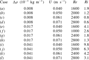
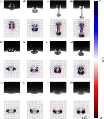
A single frame from each of the 12 cases is plotted in figure 2. The slices were selected just prior to the breakdown of the vortex-ring interaction. The ‘breakdown’ of the vortex-ring interaction refers to the generation of turbulent/chaotic motion, which is not reproducible. For each case, the density field is visualized in the upper part of each panel while the simultaneous vorticity measurements (saturated to
 $\pm 25~\text{s}^{-1}$
) are plotted in the lower part. The velocity field (vectors) is overlaid on top of the vorticity plots. The view windows measure
 $80~\text{ mm}\times 91~\text{mm}$
. While similar plots have been made previously (see Dahm et al.
Reference Dahm, Scheil and Tryggvason1989; Stock et al.
Reference Stock, Dahm and Tryggvason2008, etc.), we believe that we are the first to present simultaneous LIF/PIV measurements of the vortex-ring interaction with a stratified interface. These data will be compared with the three-dimensional results found later in this paper. Due to the low number of vortex rings, it is assumed that the density stratification does not change significantly over the course of these experiments, in agreement with Olsthoorn & Dalziel (Reference Olsthoorn and Dalziel2015).
Plot of characteristic snapshots of vortex rings interacting with a stratified interface. Images were selected just prior to the breakdown of the vortex-ring interaction. Each panel has a plot of the density at the top and the corresponding vorticity field at the bottom, with the velocity field overlaid. Vorticity values have been saturated to
 $\pm 25$
 $\text{s}^{-1}$
. Each column corresponds to a specific Reynolds number, as indicated at the top of the column. Each row corresponds to a particular density difference, as indicated on the left. The same view window was used for all panels, measuring
 $80~\text{mm}\times 91~\text{mm}$
. A small ‘
 $\times$
’ highlights the fringes identified in the text. (a,e,i)
 $Re=1600$
, (b,f,j)
 $Re=2000$
, (c,g,k)
 $Re=2400$
, (d,h,l)
 $Re=2800$
. (a–d)
 $\unicode[STIX]{x0394}\unicode[STIX]{x1D70C}=0.041~\text{g}~\text{cm}^{-3}$
, (e–h)
 $\unicode[STIX]{x0394}\unicode[STIX]{x1D70C}=0.017~\text{g}~\text{cm}^{-3}$
, (i–l)
 $\unicode[STIX]{x0394}\unicode[STIX]{x1D70C}=0.008~\text{g}~\text{cm}^{-3}$
.

These plots demonstrate two key features of the vortex-ring interaction. First, the evolution of the system is largely dominated by the Richardson number, as the ratio of the potential energy of the stratification to the kinetic energy of the vortex ring. The strong similarity between figure 2(b,h) with similar Richardson numbers but at very different Reynolds numbers should be noted. Second, the transport of the lower layer fluid,
 $\unicode[STIX]{x1D70C}_{2}$
, into the upper layer tracks with the generation of secondary vorticity by the baroclinic shear. That is, the primary vorticity in the system is that of the vortex ring, which, through interaction with the stratification, produces a secondary vorticity, which entrains the lower layer fluid. This baroclinic vorticity transfer will henceforth be denoted as BVT. Here, BVT occurs at the location of the deformed interface, where the density gradient is largest. The secondary vorticity then rolls up the density interface as it transports lower layer fluid into the upper layer. As another example of an instability with a very high mixing efficiency, we note that the Rayleigh–Taylor instability does not require BVT to produce mixing, as the statically unstable initial stratification can feed the baroclinic production of vorticity directly.
It is worth noting that, due to the finite light-sheet thickness (
 ${\sim}$
2 mm), many of the density field images demonstrate a weak background signal resulting from the three-dimensionality of the flow. In particular, the instability of the vortex ring is visible in the bright/dark fringes within the density field image (particularly noticeable in figure 2(l) located just below the ‘
 $\times$
’). We will refer back to this in § 4 when discussing the ‘phase locking’ discovered in the three-dimensional ensembles.
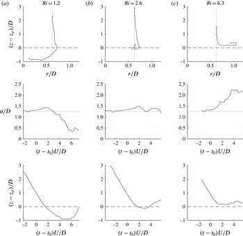
Evolution of the vortex-ring centre for
 $Re=2000$
demonstrating the penetrative (a), partially penetrative (b) and non-penetrative (c) regimes. All axes have been appropriately non-dimensionalized by the vortex tube diameter and the advective time scale.

It is important to understand how the depth of penetration of the vortex rings changes with the Richardson number. Figure 3 plots the location of the
 $Re=2000$
vortex-ring peak vorticity as a function of time. In this figure,
 $z_{\unicode[STIX]{x1D70C}}$
is the height of the unperturbed density interface, and the vortex-ring diameter,
 $a$
, is defined as the distance between vorticity centroids. In each of the cases presented, length has been non-dimensionalized by the vortex tube diameter (
 $D$
) and time has been non-dimensionalized by the advective time scale (
 $t^{\ast }=D/U$
). The time
 $t=0$
has been specified when the vortex ring is a distance
 $D$
from the unperturbed density interface. In this analysis, the vertical position of the vortex ring is defined as the mean vertical position of the two vorticity centroids of the vortex ring in the plane of the laser sheet. This definition provides a simple measure for the vortex-ring penetration depth over a significant portion of the interaction but clearly loses its meaning once the flow becomes sufficiently turbulent. In figure 3, we observe two different stratification regimes: a penetrative regime where the vortex rings are capable of penetrating into the lower layer and a non-penetrative (wall-like) regime where they are not. In (a–c), figure 3 plots typical examples of the penetrative, partially penetrative (boundary case) and non-penetrative regimes. We observe that, in all cases, as the vortex ring approaches the lower layer, the vortex-ring diameter expands, even within the penetrative regime. This is true even for the lowest-Richardson-number cases. This expansion, which will result in vortex stretching, has the potential to produce instabilities on the vortex-ring surface. Tracking of the vortex-ring core terminates once the vortex-ring interaction becomes sufficiently chaotic that the vortex ring becomes masked by the turbulent vorticity.
It is clear in figure 3 that the time scale of the interface rebound decreases with an increase in the Richardson number. The trajectory of the vortex-ring rebound is not quadratic as would be expected for a purely buoyancy-driven response of the interface. If the vortex ring penetrates into the lower layer, the ring diameter will contract until it has been ‘unwound’ by the BVT mechanism. In contrast, if the vortex ring is unable to penetrate into the lower layer, the vortex-ring diameter will expand, similarly to the results of Bethke & Dalziel (Reference Bethke and Dalziel2012). Many similarities exist between the present high-Richardson-number vortex-ring interactions and the interaction of a vortex ring with a solid wall. In both cases, there is a production of secondary vorticity under the impinging vortex ring in combination with the ring expansion. However, the mechanism of the vorticity production is different between the two cases. In the vortex-ring–wall interaction, the secondary vorticity is produced through the viscous boundary layer as a result of the no-slip wall condition. The interface boundary condition for a vortex ring impinging on a two-layer stratification is free-slip and does not lead to this viscous boundary-layer formation directly; rather, the secondary vorticity is generated via the BVT. In both cases, the secondary vorticity is ‘rolled up’ around the primary vortex, which results in the vortex breakdown.
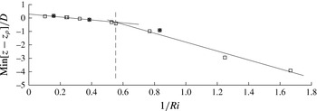
Plot of the minimum vertical position achieved by a vortex ring for all cases. Stars (*) represent the cases presented in figure 3. A dashed line has been plotted to denote the boundary between the penetrative and non-penetrative regimes.

Figure 4 plots the maximum penetration depth of the vortex-ring core for all cases. We expect to find (as in Linden Reference Linden1973) that the penetration depth is given by a balance of the kinetic energy of the vortex ring and the potential energy of the displaced density field. Specifically, we expect the penetration depth to scale as
 $1/Ri$
. A piecewise linear fit to the data (plotted as a solid line in figure 4) is given:
 $$\begin{eqnarray}\displaystyle \frac{\min [z-z_{\unicode[STIX]{x1D70C}}]}{D}=\left\{\begin{array}{@{}ll@{}}\left(-1.09\pm 0.29\right)Ri^{-1}+0.07,\quad & Ri\leqslant 1.81,\\ \left(-3.38\pm 1.53\right)Ri^{-1}+0.24,\quad & Ri>1.81.\end{array}\right. & & \displaystyle\end{eqnarray}$$
It should be noted that, due to the low number of data points, the error in the fit slopes is large. However, there is a clear division between the penetrative and non-penetrative regimes. Here, we expect the division to occur when there is a balance of potential and kinetic energy in the system,
 $Ri=O(1)$
. The experimental division point is estimated as
 $Ri=1.81$
. In the discussion of the three-dimensional vortex-ring visualizations below, we present a case within the penetrative regime
 $(Ri=0.98)$
, a case near the division point
 $(Ri=1.7)$
and a case in the non-penetrative regime
 $(Ri=2.4)$
. This separation between regimes is reminiscent of the work of Camassa et al. (Reference Camassa, Khatri, Mclaughlin, Mertens, Nenon, Smith and Viotti2013), who investigated the trapping/penetration of dense vortex rings into the lower layer of a two-layer stratification. More work is needed to expand upon the comparison between such negatively buoyant rings and our present scenario.
Linden (Reference Linden1973) argued that the rebound time scale of the vortex-ring interaction scales as a purely buoyancy-driven response, i.e.
 $Ri^{-1/2}$
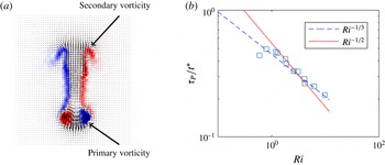
. Here, we investigate the time scale associated with the production of secondary azimuthal vorticity generated by the BVT. We argue that this is a better measure of the rebound time scale. This secondary vorticity generated by the BVT has an azimuthal component of opposite sign to the impinging vortex ring. We determine the time scale by plotting the total (volume-integrated) secondary vorticity as a function of time. The exact functional form of the baroclinic production is unknown, but a Gaussian function provides a good fit to the growth of secondary vorticity. The Gaussian fit then provides a time scale for the baroclinic production. Figure 5(a) explicitly denotes the difference between the primary and secondary (BVT-generated) vorticity. Figure 5(b) plots the rebound time scale non-dimensionalized by the advective time scale (
 $t^{\ast }$
) versus the Richardson number. We observe that the production time scale appears to scale as
 $Ri^{-1/3}$
. If the baroclinic production and interface rebound occur on the same time scale, this will directly affect the Linden (Reference Linden1973) estimate for the entrainment rate. As the primary aim of this paper is to investigate the three-dimensionality of the interaction, we do not discuss this further, but we note that the power-law exponent for the time scale of the interface rebound, in either methodology, is less than one.
Plots of (a) the vorticity field extracted from figure 2 denoting the primary and secondary vorticity and (b) the time scale associated with the baroclinic production of vorticity as a function of
 $Ri$
.

3 Three-dimensional methods
For the remainder of this discussion, we will consider vortex rings generated in a large tank (
 $0.45\times 0.45\times 0.60~\text{m}^{3}$
), with a horizontal light sheet produced by the pulsed laser. The horizontal light sheet was positioned normal to the vertically propagating vortex rings. Each laser was triggered at a rate of 75 Hz. Two cameras (Allied Vision Technologies, Bonito CMC-4000 4MP), equipped with 60 mm (
 $f/2.8$
) Nikon lenses, were positioned on opposite sides of the tank. The cameras were set to record at 150 frames per second. In order to increase the temporal resolution of the image pairs, the two laser pulses were staggered (with a pulse separation of 2 ms) about the camera frame separation. Here, 75 pairs of laser pulses were produced each second. We were able to achieve much higher temporal resolution image pairs than with an evenly spaced laser triggering. However, as a consequence of the precise laser triggering, only one velocity field could be computed for each pair of laser pulses. Thus, each second the cameras recorded 150 images, which resulted in 75 image pairs used to determine the velocity field within the flow. Both the laser and the cameras were triggered via the connected computer system, allowing for precise laser-pulse and camera-frame triggering. The cameras were additionally equipped with Scheimpflug adapters (Dantec Dynamics), which allowed both cameras to be focused onto the laser sheet within the tank. The fluid within the tank was again seeded with
 $20~\unicode[STIX]{x03BC}\text{m}$
polyamide particles. Figure 6 shows a diagram of the experimental set-up.
Diagram of the tank set-up for the horizontal laser sheet, highlighting the discharge of fluid from the tank base and the addition of fresh water to the top of the water column.

It is worth noting that there are several stark differences between the work presented here and the vertical-slice cases presented in § 2. Primarily, the laser sheet is now horizontal, with the two cameras positioned at an angle to the plane normal. The cameras were positioned facing the lateral sides of the tank to avoid the vortex tube framework. The incident angle of the cameras was low enough such that the tank walls did not substantially obscure the particle images. The incident angle was limited by the internal angle of reflection of the tank walls. As both available cameras were used for the stereo-PIV, no density information was available. As both salt solutions modified the conductivity of the fluid, the use of a conductivity probe was also cumbersome and, as such, we did not use one here. The second camera used for PIV enabled the three-dimensional reconstruction of the velocity field, which was not previously available. As the only light reaching the cameras was that scattered from the particles within the light sheet, no filters were necessary.
3.1 Stereo-PIV methodology
Each PIV camera provided a two-dimensional projection of the particles visible within the laser sheet. As a first step, the image sequence from each camera was used to compute a two-dimensional pixel-displacement field in the natural pixel coordinate system of that camera. Three coordinate systems were then needed to project this information onto the three components of velocity within the plane of the laser sheet.
The coordinate systems were constructed using a two-level calibration grid of a known geometry, placed within the focal plane window of both cameras at a known real-world position. Using this information, mappings between the pixel and world coordinates could be established. Here, we determined the two-dimensional world coordinate mapping for each camera along with a three-dimensional world coordinate system projecting the four pixel coordinates (two per camera) into three-dimensional space. Each coordinate system was constructed using a least-squares procedure from polynomial basis functions. The individual two-dimensional systems were registered to the plane of the laser sheet through an iterative process that included cross-correlating the PIV images from one camera with those from the other.
The individual two-dimensional coordinate systems were then used to map the pixel-displacement field from the pixel coordinates of each camera onto the common
 $x{-}y$
coordinates of the laser sheet so that four pixel-displacement components were known for every location in the
 $x{-}y$
plane. Finally, the Jacobian derivative matrix of the three-dimensional coordinate system mapping was used to project these four pixel displacements into the three components of the velocity field.
To verify this process, we also back-projected the three components of the velocity in the world coordinate system onto pixel displacements in the pixel coordinates of the individual cameras. Comparison of these back-projected fields with the original pixel-displacement fields from the two-dimensional PIV allowed the performance of the processing to be assessed and optimized.
3.2 Vortex-ring reconstruction
As an initial test of the stereo-PIV system, we produced vortex rings in an unstratified tank. In order to reconstruct the velocity field of the vortex ring in the homogeneous fluid, the vortex ring was assumed to be purely advected according to its propagation speed (in this case,
 $U=0.040~\text{m}~\text{s}^{-1}$
). The advective assumption states that as the vortex ring propagates, the velocity field recorded within a fixed plane normal to the direction of propagation is equivalent to the instantaneous velocity of the vortex ring in all three spatial dimensions. Under this assumption, the virtual level spacing between each frame of a camera recording is simply given by
 $\text{d}z=U\,\text{d}t$
. That is, the vertical spacing (
 $\text{d}z$
) is the product of the vortex-ring propagation speed (
 $U$
) and the time between velocity snapshots (
 $\text{d}t$
). Figure 7 provides a diagram of this reconstruction process. For these unstratified experiments, the camera capture rate was limited to 100 frames per second, resulting in 50 image pairs per second used to reconstruct the velocity field. The vertically discretized reconstruction
 $R$
is thus computed from the velocity field slices
 $I$
. The slices
 $I$
are computed from images of the physical vortex-ring flow field
 $F$
at the fixed laser-sheet height
 $z_{0}$
and the varying frame time
 $t_{f}$
, written as
 $$\begin{eqnarray}R(x,y,Ut_{f}-z_{0})=I(x,y,z_{0},t_{f})=\int F(x,y,z,t)\unicode[STIX]{x1D6FF}_{z}(z-z_{0})\unicode[STIX]{x1D6FF}_{t}(t^{\prime }-t_{f})\,\text{d}z\,\text{d}t^{\prime }.\end{eqnarray}$$
This is an idealization where
 $\unicode[STIX]{x1D6FF}_{z}$
and
 $\unicode[STIX]{x1D6FF}_{t}$
are Dirac delta functions. In practice,
 $R$
is constructed from finite width intervals where
 $\unicode[STIX]{x1D6FF}_{z}$
is the laser-sheet thickness (
 ${\approx}1~\text{mm}$
) and
 $\unicode[STIX]{x1D6FF}_{t}$
is the duration of the laser pulse (
 ${\approx}10~\text{ns}$
). The physical coordinates are given as
 $x,y,z$
. An alternative method would be to reposition the light sheet and reconstruct the vortex ring over an ensemble of experiments by appropriately time-correlating the image frames to a fixed time
 $t_{0}$
, relative to the generation time. That is, for repositioned laser-sheet height
 $z_{E}$
,
 $$\begin{eqnarray}R(x,y,Ut_{f}-z_{0})\sim \tilde{R}(x,y,z_{E})=\int F(x,y,z,t)\unicode[STIX]{x1D6FF}_{z}(z-z_{E})\unicode[STIX]{x1D6FF}_{t}(t^{\prime }-t_{0})\,\text{d}z\,\text{d}t^{\prime }.\end{eqnarray}$$
The (
 $\tilde{\,\cdot \,}$
) denotes a reconstruction assembled from an ensemble of experiments. This ensemble approach projects the data into the space of reproducible velocity field measurements. That is, chaotic or turbulent motions will be manifested as noise using this ensemble methodology. The two methods are asymptotically similar in the limit of small inter-frame spacing and level heights, provided that the motion is perfectly repeatable between realizations.
Diagram of the reconstruction algorithm from a series of horizontal slices taken with a temporal spacing
 $\text{d}t$
.

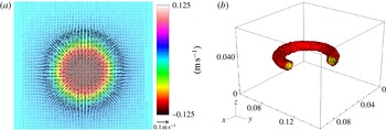
Figure 8(a) plots a single frame of the reconstructed three components of velocity within a horizontal plane. Here, the vertical velocity (out of the page) is represented by the image colours and the vectors represent the planar velocity field. Figure 8(b) then plots isosurfaces of the magnitude of the vorticity vector for the three-dimensional reconstruction. The isosurfaces are plotted at 40 % (yellow) and 25 % (red) of the maximum value of vorticity for the smoothed (using a median filter) data set. The axis dimensions are in metres. The spatial resolution of the ensemble was
 $\text{d}x\times \text{d}y\times \text{d}z=0.172\times 0.171\times 0.779~\text{mm}^{3}$
.
Three-dimensional reconstruction of a vortex ring within a homogeneous fluid. (a) The three components of velocity within a single frame. Colour represents the vertical velocity (out of the page) and arrows indicate the planar velocity field. (b) Isocontours of vorticity magnitude at 40 % (yellow) and 25 % (red) of the maximum value of vorticity for the smoothed data set. The axis dimensions are in metres.

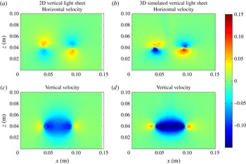
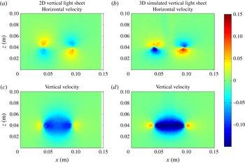
Comparison of the computed horizontal (a,b) and vertical (c,d) velocity fields within a vertical plane. (a,c) Velocity field computed from a vertical light sheet. (b,d) Velocity field computed from the reconstruction using the layering methodology.
We find excellent agreement between the three-dimensional velocity data set
 $R$
collected here and the velocity field collected from two-dimensional measurements in a vertical light sheet through the centre of a vortex ring. Figure 9 plots a comparison of the horizontal (a,b) and vertical (c,d) velocity fields determined using both a vertical light sheet (a,c) and a simulated virtual light sheet (b,d) derived from the vortex-ring reconstruction (i.e.
 $R(x,y_{0},z)$
for fixed constant
 $y_{0}$
, positioned at the centre of the vortex ring). Both the vertical light sheet and the reconstructed planes are saturated to the same values. We find good agreement in the diameter of the ring and in the velocity values. The magnitudes of the velocity fields are slightly larger in the 3D case, and the width of the vertical velocity distribution is marginally greater. The differences between the two planes can be largely explained by the vertical light sheet being slightly off-centre to the axis of the ring, which is an experimental inevitability. Additionally, we note that the change of experimental set-ups will also add to the discrepancy between velocity measurements. We believe that this comparison strongly supports the ensemble methodology.
It should be noted that we do not observe any instability occurring on the ring. The Widnall et al. (Reference Widnall, Bliss and Tsai1974) instability will eventually grow to large amplitude and cause the vortex ring to become visibly unstable. However, at the time at which the vortex ring reaches the height of the laser sheet, the instability has not had sufficient time to grow to finite amplitude. This has important implications for the work presented below.
3.3 3D field from multiple experiments
In § 2, we observe that vortex-ring interactions with a stratified interface are surprisingly robust. We take advantage of this reproducibility here. In the following work, we filled the experimental tank with a two-layer stratification. The tank was stratified as described previously. As the lower layer fluid was extracted between subsequent experiments in order to ‘slice through’ the vortex-ring interaction, the initial depth of the lower fluid layer was estimated such that the maximal penetration of the vortex ring was just above the laser sheet. Typical initial lower layer depths were of the order of 0.25 m, where the light sheet was positioned at a height of 0.19 m above the base of the tank.
Once the stratification was established, the following experimental protocol was followed.
-
(i) The laser system was activated and temporally synchronized with the cameras.
-
(ii) A vortex ring was generated.
-
(iii) The vortex-ring interaction was recorded.
-
(iv) The cameras and laser system were turned off.
-
(v) Using a peristaltic pump, a controlled volume of fluid was removed from the lower layer. Using a second peristaltic pump, fresh water was added at the top of the water column in order to conserve the total water-column height. The volume removed was 393 (
 $\pm 2$
) ml, corresponding to an interface shift of 0.0019 m.
-
(vi) A 5 min settling period was implemented from the start of the previous experiment in order for any residual motions within the water tank to diffuse.
-
(vii) The experiment was repeated.

By controlling the position of the interface through the use of two peristaltic pumps, the distance between the density interface and the laser sheet was changed. This allowed us to control the relative height of each recorded experiment in order to ‘scan through’ the vortex-ring interaction. It should be noted that figure 6 includes the extraction and input of fluid through the system.
In contrast to the unstratified case, we cannot use the propagation speed of the vortex ring to determine the spacing between level heights of the ensemble. Here, each individual realization is now time-dependent regardless of the frame of reference. By knowing the volume extracted between each vortex-ring interaction, we estimate the relative height between each experimental data plane (i.e.
 $\unicode[STIX]{x0394}z_{E}$
). As noted in Olsthoorn & Dalziel (Reference Olsthoorn and Dalziel2015), the vortex-ring-induced mixing of the interface produces an additional shift to the interface position. We account for this additional shift when computing
 $\unicode[STIX]{x0394}z_{E}$
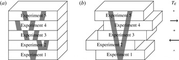
, which is approximately 5 % of the total shift. We ‘stack’ the individual experiments together, adjusting for the propagation speed of the vortex rings, in order to reconstruct the full time-resolved three-dimensional velocity field. Figure 10(a) plots a representation of this ensemble of different experiments. That is, the reconstruction
 $\tilde{R}$
is given by
 $$\begin{eqnarray}\tilde{R}(x,y,z_{E},t-T_{E})=\int F(x,y,z,t^{\prime })\unicode[STIX]{x1D6FF}_{z}(z-z_{E})\unicode[STIX]{x1D6FF}_{t}(t^{\prime }-(t-T_{E}))\,\text{d}z\,\text{d}t^{\prime }.\end{eqnarray}$$
For the purposes of the ensemble, the first experiment is assigned a vertical height of
 $z_{E}=0$
. The time synchronization between individual experiments (
 $T_{E}$
) must account for the additional time delay between the vortex-ring generation and when it reaches the laser sheet (the propagation time of the ring), as the vortex tube was fixed between experiments. In addition,
 $T_{E}$
must account for signal delays between the start of the camera capture and the generation of the vortex ring. Although hardware synchronization was used between the lasers and the camera, ensuring consistency, the synchronization between the image capture and vortex generation was software based between laboratory computers. This introduced a small random offset between different experiments of the ensemble. In order to account for this variation, the root-mean-squared (r.m.s.) value of the vertical velocity was computed over a range of frames (
 $O(1000)$
frames). Then,
 $T_{E}$
was computed as the temporal shift that provides the best correlation between subsequent experiments. Figure 10(b) plots a representation of a time-correlated ensemble. Typical
 $T_{E}$
variations are
 ${\approx}0.1~\text{s}$
, consistent with the software delay between computers. Both the level height
 $z_{E}$
and the time synchronization
 $T_{E}$
are functions of the discrete vortex-ring experiment number.
Diagram of the three-dimensional velocity reconstruction from a series of vortex-ring interaction experiments. (a) The ‘stacking’ of individual experiments in order to capture the full three-dimensional dynamics. (b) The ensemble once the experiments have been time-correlated according to their r.m.s. values to produce a consistent data set. The arrows on the right represent variations in the time synchronization
 $T_{E}$
.

In this paper, three ensembles are presented. Each ensemble was filtered using a spectral and smoothing filter. The parameters associated with these ensembles are presented in table 3. The advective time scale is given as
 $t^{\ast }$
. Density differences are restricted to small values due to the difficulties of maintaining matched refractive indices at larger density differences. The quantities
 $n_{x},n_{y},n_{z}$
and
 $\text{d}x,\text{d}y,\text{d}z$
are the grid size and grid spacing respectively. It should be noted that the last quantity
 $n_{z}$
denotes the number of experiments used to construct each ensemble. The horizontal resolution was subsampled using a cubic spline in order to facilitate the computations.
Table of the three cases used for three-dimensional velocity field reconstruction of the vortex-ring interaction.

3.4 Limitations of the methodology
A number of assumptions have been made when developing the current methodology. The primary assumption is that, throughout these experiments, the vortex rings are highly reproducible. This assumption has been validated by looking at the propagation speed of vortex rings produced within a vertical light sheet. This assumption is also supported by the high degree of correlation between neighbouring members of each ensemble. We additionally attempt to control the variation of these parameters by ensuring that the water-column height remains fixed when discharging the lower layer fluid. The second assumption is that the vortex-ring interaction dynamics are also reproducible. As we will show later in § 4, not only are the dominant axisymmetric dynamics reproducible, but we capture the resultant instabilities of the interaction. Third, the change in stratification between vortex-ring interactions does not substantially change the dynamics. The correlation of the r.m.s. values defined previously suggests that the dynamics are not substantially affected by the small perturbations to the density field. In addition, as shown in Olsthoorn & Dalziel (Reference Olsthoorn and Dalziel2015), the mixing rate associated with the vortex-ring interactions is near constant. Finally, and potentially the greatest source of error in this methodology, is the assumption that the stratification gradient is not the dominant control parameter of this problem. While the interface thickness is sharp, an exact density profile could not be determined due to the method used to match refractive indices. Here, we assume, again with reference to Olsthoorn & Dalziel (Reference Olsthoorn and Dalziel2015) for supporting evidence, that this does not have a dominant effect on the interaction.
It should be reiterated that the methodology presented here will only produce a coherent ensemble when the vortex-ring interaction is sufficiently reproducible. Of course, the vortex-ring interaction will eventually break down into turbulent motion. This turbulent motion is similar to that of a plume/fountain but will not be studied here. As we will show below, the ensemble will eventually become incoherent once the turbulent motion dominates. However, as will also be shown below, the instability itself is remarkably robust and is clearly captured by the ensemble.
4 Results
From the experiments described above, the resultant ensembles are fully three-dimensional time-resolved velocity field measurements for the evolution of the vortex-ring interactions. Unfortunately, due to the need for precise refractive-index matching of the density stratification, we do not have access to the evolution of the density field. However, the stratification methodology is similar to that found in § 2, and, in reference to figure 2, the interface thickness will be much smaller than the vortex-ring diameter. Vortex rings have also been shown to sharpen density interfaces (Olsthoorn & Dalziel Reference Olsthoorn and Dalziel2015).
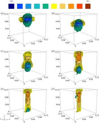
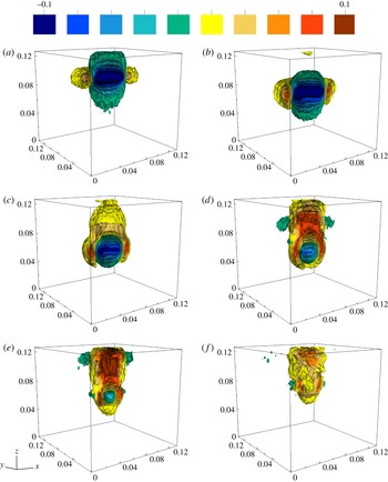
Case 1: 10 isosurfaces of vertical velocity evenly spaced between
 $-0.1$
and
 $0.1~\text{m}~\text{s}^{-1}$
. The contours are plotted at (a)
 $t=0.00~\text{s}$
, (b)
 $t=1.00~\text{s}$
, (c)
 $t=2.00~\text{s}$
, (d)
 $t=$
 $3.00~\text{s}$
, (e)
 $t=4.00~\text{s}$
and (f)
 $t=5.00~\text{s}$
. The data have been cropped about the centre (
 $y=0.07~\text{m}$
) of the vortex ring in order to visualize the core dynamics. All axes are scaled in metres.

4.1 Case 1 – penetrative –
$Re=1600$
,
$Ri=0.98$


We begin with a discussion of case 1 (
 $Re=1600$
,
 $Ri=0.98$
). Figure 11 plots three-dimensional projections of 10 evenly spaced isosurfaces of vertical velocity, between
 $-0.1$
and
 $0.1~\text{m}~\text{s}^{-1}$
, over the evolution of the interaction. Here, the plots have been generated at (a)
 $t=0.00~\text{s}$
, (b)
 $t=1.00~\text{s}$
, (c)
 $t=2.00~\text{s}$
, (d)
 $t=3.00~\text{s}$
, (e)
 $t=4.00~\text{s}$
and (f)
 $t=5.00~\text{s}$
. It should be noted that the arbitrary time origin of these data corresponds to the first plane presented. The data have been sliced through the centre of the vortex ring in order to visualize the core dynamics.
The Richardson number of case 1 is well within the penetrative regime (see § 2), and as such the penetration depth of the vortex ring into the lower layer is significant. We observe the incoming vortex ring in figure 11(b). Through the BVT, the vortex ring is slowly ‘unwound’, as seen in figure 11(c), where the vortex ring core slowly shrinks over time. The remaining panels, figure 11(d–f), plot the slow recovery of the interface. (It should be noted that the vortex ring penetrates slightly deeper than the visualization domain.)
The parameters associated with this ensemble are similar to those of the vertical-slice case presented in figure 2(f). Indeed, the vertical velocity in figure 2(f) is nearly identical to figure 11(e). Thus, the vertical-slice results provide a validation of the layering methodology of the ensemble. We note that the ensemble has a lower signal-to-noise ratio than the vertical-slice results. This error is partially a result of the inter-generational variation of the vortex rings. The experimental difficulties introduced by the non-normal camera angle and the imperfectly matched refractive indices of the two fluid layers will produce additional sources of error. Thermal and other residual motion within the tank may also contribute to the noise in the ensemble. Finally, as we mentioned above, once the vortex-ring interaction breaks down into turbulence, the image recordings will contain data that may be identified as noise in the ensemble. However, the velocity field remains surprisingly coherent until late times of the interaction, and is more than sufficient to analyse the growth of the three-dimensional instability of the flow.
4.2 Case 2 – partially penetrative –
$Re=2400$
,
$Ri=1.7$


The parameters of case 2 present both a higher Reynolds number and a higher Richardson number (
 $Re=2400$
,
 $Ri=1.7$
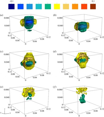
) than case 1. Figure 12 plots the same 10 evenly spaced isosurfaces of vertical velocity as used in figure 11. The contours are plotted at (a)
 $t=0.00~\text{s}$
, (b)
 $t=0.67~\text{s}$
, (c)
 $t=1.33~\text{s}$
, (d)
 $t=2.00~\text{s}$
, (e)
 $t=2.67~\text{s}$
and (f)
 $t=3.33~\text{s}$
. As for case 1, we observe the incoming vortex ring in figure 12(b). The penetration of the vortex ring into the lower layer is increasingly restricted due to the significantly higher Richardson number. We observe the corresponding rebound of the interface in figure 12(d,e). Figure 12(f) was selected to demonstrate that once the coherent nature of the vortex-ring dynamics break down into turbulent motions, the coherence of the visualizations also breaks down.
Case 2: plot of 10 isosurfaces of vertical velocity evenly spaced between
 $-0.1$
and
 $0.1~\text{m}~\text{s}^{-1}$
. The contours are plotted at (a)
 $t=0.00~\text{s}$
, (b)
 $t=0.67~\text{s}$
, (c)
 $t=1.33~\text{s}$
, (d)
 $t=2.00~\text{s}$
, (e)
 $t=2.67~\text{s}$
and (f)
 $t=3.33~\text{s}$
. The data have been cropped about the centre (
 $y=0.07~\text{m}$
) of the vortex ring in order to visualize the core dynamics. All axes are scaled in metres.

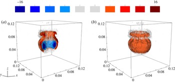
In this paper, we primarily focus on the evolution of the vortex-ring velocity field due to its smoothness. However, figure 13 plots 10 isosurfaces of the azimuthal component of vorticity at
 $t=2.00~\text{s}$
saturated at
 $\pm 25~\text{s}^{-1}$
. Figure 13(a) plots the vorticity, which has been sliced through the ring centre in order to view the core dynamics and to make a comparison with the vertical-slice experiments with similar parameter values (see figure 2
g). It is clear that the ensemble approach and the vertical-slice images are in qualitative and quantitative agreement (the isosurfaces have been saturated to the same value as that of figure 2). Figure 13(b) plots the identical data without the mid-plane slicing such that the three-dimensionality of the interaction can be seen. There exists a clear modal instability in the azimuthal direction. Here, the vorticity generated by the BVT is plotted in red. A discussion of the instability is provided below. However, we note here that the instability is occurring on the baroclinically generated vorticity that is of the same mode number as would be observed in the primary vorticity of the unstratified vortex ring (there is no secondary vorticity in that case).
Case 2: plot of 10 isosurfaces of azimuthal vorticity, bounded by
 $\unicode[STIX]{x1D714}_{\unicode[STIX]{x1D703}}=\pm 25~\text{s}^{-1}$
. Contours are plotted at
 $t=2.00~\text{s}$
. (a) Plot of the vorticity sliced through the centre of the ring. (b) The identical vorticity plot without slicing.

It is worth noting that the Richardson number of case 2 is near the boundary between the penetrative and non-penetrative regimes discussed in § 2.
4.3 Case 3 – non-penetrative –
$Re=1600,Ri=2.4$

Case 3 has an identical Reynolds number to case 1 but with a higher Richardson number (
 $Re=1600,Ri=2.4$
). As with figures 11 and 12, figure 14 plots 10 evenly spaced isosurfaces of vertical velocity, between
 $-0.1$
and
 $0.1~\text{m}~\text{s}^{-1}$
, over the evolution of the interaction. The contours are plotted at intervals of 1 s. The evolution of the vortex ring observed here is similar to that for the previous two cases.
Case 3: plot of 10 isosurfaces of vertical velocity evenly spaced between
 $-0.1$
and
 $0.1~\text{m}~\text{s}^{-1}$
. The contours are plotted at (a)
 $t=0.00~\text{s}$
, (b)
 $t=1.00~\text{s}$
, (c)
 $t=2.00~\text{s}$
, (d)
 $t=3.00~\text{s}$
, (e)
 $t=4.00~\text{s}$
and (f)
 $t=5.00~\text{s}$
. The data have been cropped about the centre (
 $y=0.07~\text{m}$
) of the vortex ring in order to visualize the core dynamics. All axes are scaled in metres.

The vertical-slice case that most closely corresponds to the Richardson number of case 3 is plotted in figure 2(f). As case 3 is within the non-penetrative regime, we do not observe a shrinking of the vortex-ring diameter during the vortex-ring interaction but rather its expansion (see figure 14 c,d). Despite the much higher Richardson number, the mode of instability in the velocity field is identical for cases 1 and 3, which have the same Reynolds number. We return to this later.
It is remarkable that the vortex-ring interaction with a stratified interface is as repeatable as shown here. In the three cases presented above, the vortex-ring dynamics are encapsulated by the ensemble until relatively late stages of the interaction despite the breakdown of the axisymmetry. Indeed, the ensemble captures the initial growth of the instability as well as the bulk dynamics of the flow. The instability itself appears to be phase-locked and does not require rotation of the individual realizations about the
 $z$
-axis as was originally expected. This phase locking, discussed below, may be a result of non-circular perturbations to the base of the vortex tube (measured to be
 $0.64\pm 0.13\,\%$
of the vortex tube diameter), which are of sufficiently small amplitude that their effect is not visible in the homogeneous case. As we will continue to show below, the consistency of the vortex-ring interaction is surprising beyond any initial estimates. In the context of stratified mixing, this may suggest that individual turbulent eddy mixing events may be substantively more repeatable than previously thought. We hope that future work will be performed to quantify this repeatability in a turbulent context.
4.4 Three-dimensional instability
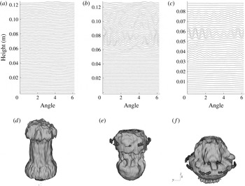
In the absence of stratification, Maxworthy (Reference Maxworthy1977) noted the appearance of definitive peaks and troughs in the dye entrained by a vortex ring. He associated these modes with solitary waves forming on the surface of the vortex ring. It was then shown that the mode number of the vortex-ring waves depends on the Reynolds number alone, for low Reynolds numbers (Maxworthy Reference Maxworthy1977; Saffman Reference Saffman1978). We do not observe any evidence of this instability on a vortex ring within an unstratified fluid, at the position of the laser sheet. However, for the stratified cases, figure 15 plots a 0.01 m thick horizontal slice of six isosurfaces of vertical velocity for all three ensembles for case 1 at
 $t/t^{\ast }=3.76$
, case 2 at
 $t/t^{\ast }=4.18$
and case 3 at
 $t/t^{\ast }=3.76$
. These slices were positioned just above the downward propagating vortex ring in order to demonstrate the dominant instability in the vertical velocity field. The mode number of the instability, for each case, can be identified as (a) case 1 (
 $Re=1600$
), mode 8, (b) case 2 (
 $Re=2400$
), mode 10 and (c) case 3 (
 $Re=1600$
), mode 8. We see that the mode number of the instability is indeed dictated by the Reynolds number. The mode of the unstratified vortex-ring instability (Widnall et al.
Reference Widnall, Bliss and Tsai1974) is estimated as
 $n\approx$
9 in all three cases. This agrees well with the present observations in a stratified environment. We note that the instability is predominantly expressed in the secondary vorticity field generated through the BVT. We also point out that the uneven nature of the instability is viewed elsewhere for vortex rings travelling in an unstratified medium (Krutzsch et al.
Reference Krutzsch, Bolster, Hershberger and Donnelly1939).
Representative 0.01 m slices of vertical velocity are plotted to demonstrate the interaction instability. The time of each ensemble slice is as follows: (a) case 1 at
 $t/t^{\ast }=3.76$
(
 $t=3.67~\text{s}$
), (b) case 2 at
 $t/t^{\ast }=4.18$
(
 $t=2.67~\text{s}$
) and (c) case 3 at
 $t/t^{\ast }=3.76$
(
 $t=3.67~\text{s}$
).

(a–c) Waterfall plots of the angular distribution of vertical velocity by level height. (d–f) Two isosurfaces of the vertical velocity field, highlighting the three-dimensional structure. It should be noted that the phase reversal is clearly visible in all three panels. From (d) to (f), the panels plot the ensembles corresponding to cases 1, 2 and 3. The time at which each plot is taken is identical to figure 15.

In addition to the mode number, figure 15 highlights that increasing the Richardson number of a vortex-ring interaction increases the maximum amplitude of the instability as well as the complexity (or structure) of the perturbations. With reference to figure 15(c), the structure of this instability is reminiscent of the numerical results found by Archer et al. (Reference Archer, Thomas and Coleman2008) and Feng, Kaganovskiy & Krasny (Reference Feng, Kaganovskiy and Krasny2009) in the absence of stratification. It should be noted that the instability appears to be all but absent in the work of Stock et al. (Reference Stock, Dahm and Tryggvason2008) for the numerical simulation of a vortex ring impacting a stratified interface. The similarity of the results presented in this paper with the numerical studies of unstratified vortex rings, along with the theoretical results of Widnall et al. (Reference Widnall, Bliss and Tsai1974), Maxworthy (Reference Maxworthy1977) and Saffman (Reference Saffman1978), is suggestive that there is a strong correlation between the unstratified and stratified instability mechanisms. However, it is clear that the stratification does affect the growth of the vortex-ring instability, catalysing the growth of waves on the secondary vorticity surface. This stratification-enhanced growth is consistent with the work of Atta & Hopfinger (Reference Atta and Hopfinger1989), who showed that vortex-ring instabilities occurred substantially earlier in a stratified environment than in the corresponding unstratified case. Figure 3 demonstrates that vortex rings expand as they approach the density interface. This expansion, similar to that found for a vortex ring impacting a free-slip surface, can enhance the instability (see Archer et al. Reference Archer, Thomas and Coleman2009).
In order to investigate the instability of the vortex-ring interaction, the azimuthal coordinate,
 $\unicode[STIX]{x1D703}$
, was divided into 50 bins,
 $\unicode[STIX]{x1D703}_{i}$
, from which the angular distribution of vertical velocity,
 $P(z,t)$
, was computed,
 $$\begin{eqnarray}P_{j}(z,t)=\sqrt{\frac{\displaystyle \int _{0}^{R}\int _{\unicode[STIX]{x1D703}_{j}}^{\unicode[STIX]{x1D703}_{j}+(2\unicode[STIX]{x03C0}/50)}\left(w^{2}-\langle w\rangle ^{2}\right)r\,\text{d}r\,\text{d}\unicode[STIX]{x1D703}}{\displaystyle \int _{0}^{R}\int _{\unicode[STIX]{x1D703}_{j}}^{\unicode[STIX]{x1D703}_{j}+(2\unicode[STIX]{x03C0}/50)}r\,\text{d}r\,\text{d}\unicode[STIX]{x1D703}}}.\end{eqnarray}$$
The angled brackets denote the horizontal mean. The finite extent of the ensemble domain restricts the radial extent of the integration
 $R$
, here selected to be
 $R=0.05~\text{m}$
. Figure 16 is a waterfall plot of
 $P_{j}$
versus
 $\unicode[STIX]{x1D703}$
for the same output times as figure 15. We observe the striking phenomenon that in all three ensembles there exists a phase locking of the instability between consecutive experiments of the ensemble. Specifically, the instability is rotationally aligned over many different experiments (each
 $z$
is here from a different experiment of the ensemble) of a particular parameter case. Evidence from the vertical laser-sheet experiments in § 2, performed in a smaller tank, suggests that the phase-locking phenomenon is not a result of the tank domain. It is possible that small non-circular perturbations on the inside of the tube used to generate the vortex rings may be the cause of the phase locking. However, the orientation of the instability is not constant for different ensembles (see below). Regardless of how the phase locking is occurring, the phase locking does not control the wavenumber of the instability.
Recent experimental measurements of unstratified vortex rings (Ponitz et al. Reference Ponitz, Sastuba and Brücker2015) have demonstrated that the unstratified instability is stationary (i.e. no azimuthal propagation) at early times. Indeed, this agrees with both the prediction of Widnall et al. (Reference Widnall, Bliss and Tsai1974) and the numerical results of Archer et al. (Reference Archer, Thomas and Coleman2008). Thus, we suggest that the vortex-ring instability in the stratified environment should be similarly stationary. Indeed, we do not observe any azimuthal propagation of the wave structures in the ensembles.
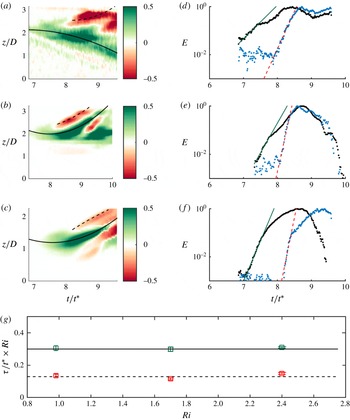
Plots are presented for case 1 (a,d), isolating the mode-8 signal, case 2 (b,e), isolating the mode-10 signal, and case 3 (c,f), isolating the mode-8 signal. Panels (a–c) plot
 $A\cos [\unicode[STIX]{x1D719}-\unicode[STIX]{x1D719}_{0}]$
for a case-specific constant
 $\unicode[STIX]{x1D719}_{0}$
versus time. Here, the colour is an indication of the amplitude of the instability. Panels (d–f) plot the energy associated with the two instabilities (identified by black lines) versus time. The scaled time scales associated with the instability growth are plotted versus the Richardson number in (g). Plots (b), (d) and (f) are normalized to unity.

With reference to the phase locking, we observe the existence of a phase reversal of
 $P$
(determined from the vertical velocity) at various heights. This phenomenon is observed for all three cases. As discussed above, this phase reversal is not a result of an angular phase speed of the instability. Figure 16(d–f) plots the associated three-dimensional structure of the vertical velocity, which demonstrates the phase reversal of the instability. Figure 13(b) also plots this phase reversal in the secondary vorticity field. It should be noted that we are only looking at one component of the velocity in
 $P$
. The instability can rotate into
 $u$
then back into
 $w$
. This phase reversal is not entirely understood. One explanation is that as the instability of the secondary vorticity field grows, it is also being advected. This advection causes the sheet of secondary vorticity to ‘roll up’ on itself, producing an apparent reversal. More work needs to be done to understand this phenomenon.
We observe that the dominant instability is of a single mode number. From the angular distribution of vertical velocity, which was sampled at points
 $j$
, we compute the Fourier transform of each level height
 $z_{a}$
as
 $$\begin{eqnarray}P_{j}(z_{a},t)=\mathop{\sum }_{k}c_{k}(z_{a},t)\exp \left[\text{i}k\unicode[STIX]{x1D703}_{j}\right].\end{eqnarray}$$
For the dominant instability mode
 $n$
, we write the corresponding complex Fourier coefficient in polar form,
 $c_{n}=A\text{e}^{\text{i}\unicode[STIX]{x1D719}}$
, for real coefficients
 $A,\unicode[STIX]{x1D719}$
. A median filter was applied to both coefficients. In order to distinguish between the phase-reversed instabilities, figure 17(a–c) plots
 $A(z)\cos [\unicode[STIX]{x1D719}(z)-\unicode[STIX]{x1D719}_{0}]$
as a function of time, for the case-dependent constant
 $\unicode[STIX]{x1D719}_{0}$
. The parameter
 $\unicode[STIX]{x1D719}_{0}$
was selected such that
 $\cos [\unicode[STIX]{x1D719}(z)-\unicode[STIX]{x1D719}_{0}]=1$
, where
 $A(z)$
is maximized. In the current coordinate system, the values of
 $\unicode[STIX]{x1D719}_{0}$
are given by
 $$\begin{eqnarray}\text{case 1, }\frac{\unicode[STIX]{x1D719}_{0}}{\unicode[STIX]{x03C0}/2}=-0.44;\quad \text{case 2, }\frac{\unicode[STIX]{x1D719}_{0}}{\unicode[STIX]{x03C0}/2}=0.56;\quad \text{case 3, }\frac{\unicode[STIX]{x1D719}_{0}}{\unicode[STIX]{x03C0}/2}=-0.34.\end{eqnarray}$$
Figure 17(a–c) differentiates between the phase-reversed instabilities by plotting
 $A\cos [\unicode[STIX]{x1D719}-\unicode[STIX]{x1D719}_{0}]$
. The two dominant instabilities are highlighted with black lines on the corresponding panels (a–c). The total energy of the identified instability (i.e.
 $E=\int \!A^{2}\unicode[STIX]{x1D6F7}_{i}(A)\,\text{d}z$
, for weighted Heaviside filter function
 $\unicode[STIX]{x1D6F7}_{i}$
) is then plotted in figure 17(d–f). These plots visualize the growth of the instability as a function of time. Linear stability theory suggests that, at early times, the dominant instability should grow as an exponential. For each instability,
 $E$
was fitted to an exponential, written as
 $$\begin{eqnarray}L=\unicode[STIX]{x1D6FC}\exp \left[\frac{t}{\unicode[STIX]{x1D70F}}\right].\end{eqnarray}$$
This method identifies a time scale (
 $\unicode[STIX]{x1D70F}$
) associated with the instability growth. The fits are then overlaid onto the appropriate panels, with the solid line plotting the fit for the dominant instability and the dashed line plotting the fit for the phase-reversed instability (corresponding to the respective phases in panels a–c). All plots are normalized by their maximum value. We note that computation of the time scale from the peak values of the mode instability energy, rather than the integrated measure, provides similar results.
As the stratification is modifying the growth of the instability, we suggest that the time scale of the instability growth should be a function of the Richardson number. Figure 17(g) plots
 $\unicode[STIX]{x1D70F}$
for each case, non-dimensionalized by the advective time scale and scaled by the Richardson number. Under this scaling, a constant line indicates an inverse Richardson number dependence, specifically
 $$\begin{eqnarray}\frac{\unicode[STIX]{x1D70F}}{t^{\ast }}\sim \frac{1}{Ri}.\end{eqnarray}$$
The data agree well with the plotted horizontal lines at time scale values of 0.30 and 0.13. The dominant and phase-reversed instabilities have different total growth rates but they both have the same Richardson number dependence. While there are only six data points at three different parameter values, the good agreement between the data and the lines is highly suggestive. Linden (Reference Linden1973) argues that the time scale associated with the rebound of the vortex-ring interaction should scale as
 $Ri^{-1/2}$
. Figure 5 supports the conclusion that the time scale power-law coefficient is less than one. This work predicts that the vortex-ring instability will grow faster than the time required for the interface to rebound when
 $Ri>1$
, allowing for the development of non-axisymmetric waves on the vortex ring. When
 $Ri<1$
, the interface will rebound prior to the development of the vortex-ring instabilities. The weak instability amplitude of case 1 (
 $Ri=0.98$
) supports this conclusion. The damping of the vortex-ring instability, when
 $Ri<1$
, may explain the drop in mixing efficiency at low
 $Ri$
suggested in Olsthoorn & Dalziel (Reference Olsthoorn and Dalziel2015).
4.5 Linear stability
As the mode number of the observed instability is the same as the unstratified vortex-ring instability, it is tempting to assert that the instability mechanism is essentially a Widnall instability. However, for the case of a vortex dipole impacting a solid wall, Harris & Williamson (Reference Harris and Williamson2012) have argued that the observed instability of the boundary-layer-produced vorticity is actually a Crow-like instability. A Crow instability produces a simple displacement mode of the vortex tube. The theoretical basis for this argument was derived from Bristol et al. (Reference Bristol, Ortega, Marcus and Savaş2004), who studied the stability of a vortex dipole of uneven circulation. The analysis shows that the Crow instability has a higher growth rate than the Widnall instability once the ratio of circulations becomes less than approximately
 $0.1$
. The wavenumber of the Crow instability is then comparable to the Widnall instability for a symmetric dipole. In addition, the instability grows more rapidly on the weaker vortex. For these reasons, Harris & Williamson (Reference Harris and Williamson2012) concluded that the observed instability of the secondary vorticity field is Crow-like.
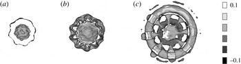
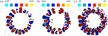
Slices of the perturbations from axisymmetric for (a) vertical velocity (
 $\text{m}~\text{s}^{-1}$
), (b) radial velocity (
 $\text{m}~\text{s}^{-1}$
) and (c) azimuthal vorticity
 $1~\text{s}^{-1}$
at
 $t=2.00~\text{s}$
(see figure 13). Slices are taken from case 2 and are defined for
 $z\in [0.077~\text{m},0085~\text{m}]$
.

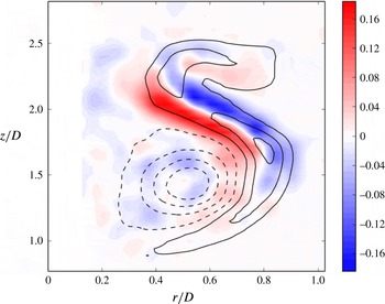
Plot of the normalized structure
 $f(r,z)$
of the instability at
 $t=2.00~\text{s}$
. Ten evenly spaced contours of the mean azimuthal vorticity field have been overlaid for comparison, highlighting the primary vortex (dashed lines) and secondary vorticity (solid lines) fields.

In the present scenario, the problem is further complicated by the effects of stratification and the curvature of the ring. As such, a more thorough investigation of the observed instability than will be presented here is warranted. However, in order to demonstrate the nature of the underlying instability, we investigate the structure of the non-axisymmetric flow field of the instability. By removing the azimuthally averaged value, figure 18 plots slices of the non-axisymmetric perturbations to the vertical velocity (figure 18
a), the radial velocity (figure 18
b), and the azimuthal vorticity (figure 18
c). All data were taken from case 2 at time
 $t=2.00~\text{s}$
(see figure 13). We see that there is no strong azimuthal dependence to the radial structure to either the vertical or radial velocity perturbations. That is, the perturbation field
 $\unicode[STIX]{x1D714}_{\unicode[STIX]{x1D716}}$
can be written as
 $$\begin{eqnarray}\unicode[STIX]{x1D714}_{\unicode[STIX]{x1D716}}=f(r,z)\cos (m\unicode[STIX]{x1D703}+\unicode[STIX]{x1D719}),\end{eqnarray}$$
for azimuthal wavenumber
 $m$
. In a manner similar to § 4.4, we can use a Fourier transform for the azimuthal vorticity to get the structural form of
 $f(r,z)$
. Figure 19 plots
 $f(r,z)$
corresponding to the mode of the instability mechanism. We observe that there is a weak signal of the Widnall instability occurring within the vortex ring. However, the signal of this vortex-ring instability is much smaller than that of the secondary vorticity field generated by the BVT. The perturbations to the azimuthal component of the secondary vorticity field are characteristic of a simple displacement mode. Both the Crow instability and the instability observed here are characterized by a displacement mode. However, it should be noted that this does not fully resolve the nature of the instability. The ‘S-shaped’ distribution differs from the circular core model of Bristol et al. (Reference Bristol, Ortega, Marcus and Savaş2004), and prevents a direct comparison of the growth rates. Future work will further investigate the effect of the stratification on the instability, and, subsequently, how the stratification modifies the growth rate.
A full characterization of the observed instability will help us to understand the vortex-ring mixing mechanism. Once the mixing of a single vortex ring has been understood, application of this work to a soup of vortex rings will help to describe the mixing efficiency observed in a turbulent environment. This work presents a first step in understanding the mixing produced by a single eddy in a chaotic system.
5 Conclusion
This study presents fully three-dimensional time-resolved ensembles encapsulating the interaction of a vortex ring with a stratified interface. We present three of these ensembles. This work demonstrates the robust and repeatable nature of the evolution of the velocity field, including the development and growth of a three-dimensional instability. This methodology is consistent with the measured vertical-slice data.
The ensembles indicate that the mode number of the vortex-ring instability in the presence of a stratified interface is consistent with the unstratified vortex-ring instability. At early times where the unstratified case shows no finite amplitude instability, the presence of stratification amplifies and catalyses the instability. The time scale of the instability growth decreases with increasing Richardson number. We suggest an inverse Richardson number dependence for the instability time scale. The structure of this instability has been characterized, and corresponds to a displacement mode of the secondary vorticity field in a manner reminiscent of the Crow instability.
The ability to achieve full three-dimensional time-resolved velocity field measurements for vortex-ring instabilities represents important progress in experimental fluid dynamics. Future work will see the integration of the present work with numerical methods to provide valuable insight into the mixing and dissipation rates of the vortex-ring evolution.
Acknowledgements
We would like to give special thanks to Y. Achache for helping the authors during the initial trials of these experiments. Support for this work was provided by the Natural Sciences and Engineering Research Council of Canada (NSERC) and through the Engineering and Physical Sciences Research Council (EPSRC). Additional support has been provided by the EPSRC Mathematical Underpinnings of Stratified Turbulence grant EP/K034529/1. Portions of the data associated with this paper can be found in the repository https://doi.org/10.17863/CAM.8284.