


1. Motivation
Singularities play a key role in fluid mechanics (Eggers Reference Eggers2018). While singularities in the form of shocks are well understood for the compressible Euler equations and the inviscid Burgers equation (Burgers Reference Burgers1948) as a simplified model, the occurrence of singularities that develop in finite time is discussed controversially for the three-dimensional incompressible Euler equations. The occurrence of singularities is strongly related to anomalous dissipation of kinetic energy in three-dimensional incompressible Euler flows, according to the pioneering work of Onsager (Reference Onsager1949), which is well documented in review articles (Eyink & Sreenivasan Reference Eyink and Sreenivasan2006; Eyink Reference Eyink2008) and in the recent essay by Dubrulle (Reference Dubrulle2019). Due to the relation between singularities and dissipation, we distinguish between (i) a direct approach to identify finite-time singularities for incompressible Euler flows, e.g. by showing that the vorticity blows up in finite time through different methods (e.g. an analysis of the kind  $\Vert \boldsymbol {\omega } \Vert _{\infty } \sim (t_* - t)^{-\gamma }$ according to the Beale–Kato–Majda theorem (Beale, Kato & Majda Reference Beale, Kato and Majda1984) trying to identify
 $t_*$ and
 $\gamma$ from numerical results), and (ii) an indirect approach providing indications of finite-time singularities by observing an ‘anomalous’ dissipative behaviour in the kinetic energy evolution. While most approaches in the literature can be identified as belonging to the first category, the present work focuses on a technique related to the second category. As explained below, this indirect approach is rather new or unexplored due to certain subtleties with respect to numerical discretisation schemes. To complement these results, we additionally show numerical results related to the direct identification approach, such as the temporal evolution of the maximum vorticity
 $\Vert \boldsymbol {\omega } \Vert _{\infty }$ and the enstrophy
 $\mathcal {E}$.
1.1. State of the art and limitations in tracing finite-time singularities
A strategy to identify potential singularities directly is that of time series expansions (Taylor & Green Reference Taylor and Green1937; Morf, Orszag & Frisch Reference Morf, Orszag and Frisch1980; Brachet et al. Reference Brachet, Meiron, Orszag, Nickel, Morf and Frisch1983; Pelz & Gulak Reference Pelz and Gulak1997), but it has been found that numerical inaccuracies prevent a definite answer when using this technique. Numerical investigations by means of partial differential equation (PDE) solvers have therefore played the most dominant role in the exploration of finite-time singularities, as detailed below.
A difficulty in identifying singularities with the direct approach by numerical simulations is the inherent conflict that arbitrarily small structures cannot be resolved with a numerical simulation of finite resolution, which renders this problem one of the most challenging topics in computational fluid dynamics. Much work has been done in this field. In the 1980s and 1990s, several early works on direct numerical simulation of both inviscid and high-Reynolds-number viscous incompressible flows reported indications of finite-time singularities for the incompressible Euler equations (Brachet et al. Reference Brachet, Meiron, Orszag, Nickel, Morf and Frisch1983; Kerr & Hussain Reference Kerr and Hussain1989; Brachet et al. Reference Brachet, Meneguzzi, Vincent, Politano and Sulem1992; Kerr Reference Kerr1993; Boratav & Pelz Reference Boratav and Pelz1994). Symmetry in the initial conditions plays an important role, as specifically mentioned and addressed in some works (Boratav & Pelz Reference Boratav and Pelz1994; Pelz & Gulak Reference Pelz and Gulak1997; Pelz Reference Pelz2001), raising the question of whether singularities are possible for problems that are not perfectly symmetric. However, these works do not allow a definite answer to the question of finite-time singularities; see also the review articles on this topic (Gibbon Reference Gibbon2008; Hou & Li Reference Hou and Li2008). One of the main reasons why the results of these studies have been inconclusive is that the spatial resolution has been limited due to the computational power and computational approaches available at the time. Numerical results shown in Hou & Li (Reference Hou and Li2008) suggest that dynamic depletion of vortex-stretching could be a mechanism that prevents a finite-time blowup, but the same authors report evidence for a finite-time singularity for a different flow configuration with solid boundaries in a later work (Luo & Hou Reference Luo and Hou2014).
In terms of the flow configuration being studied, numerical investigations on finite-time singularities can be categorised as follows. The Taylor–Green vortex has been analysed in Brachet et al. (Reference Brachet, Meiron, Orszag, Nickel, Morf and Frisch1983), Brachet et al. (Reference Brachet, Meneguzzi, Vincent, Politano and Sulem1992), Brachet (Reference Brachet1991), Shu et al. (Reference Shu, Don, Gottlieb, Schilling and Jameson2005), Cichowlas & Brachet (Reference Cichowlas and Brachet2005) and Bustamante & Brachet (Reference Bustamante and Brachet2012), and for a regularised problem considering the Euler–Voigt equations in Larios et al. (Reference Larios, Petersen, Titi and Wingate2018); the high-symmetry Kida–Pelz initial condition in Hou & Li (Reference Hou and Li2008), Cichowlas & Brachet (Reference Cichowlas and Brachet2005) and Grafke et al. (Reference Grafke, Homann, Dreher and Grauer2008); colliding Lamb dipoles in Orlandi, Pirozzoli & Carnevale (Reference Orlandi, Pirozzoli and Carnevale2012); and other perturbed cylindrical vortex tubes in Kerr & Hussain (Reference Kerr and Hussain1989), Kerr (Reference Kerr1993), Hou & Li (Reference Hou and Li2008), Grauer, Marliani & Germaschewski (Reference Grauer, Marliani and Germaschewski1998) and Kerr (Reference Kerr2013). Most studies use spectral methods as discretisation schemes.
For these direct numerical simulations, common approaches to trace singularities are monitoring the maximum vorticity  $\Vert \boldsymbol {\omega } \Vert _{\infty }$ over time (see the Beale–Kato–Majda theorem (Beale et al. Reference Beale, Kato and Majda1984)) and the ‘analyticity strip’ method (see Sulem, Sulem & Frisch Reference Sulem, Sulem and Frisch1983), which aims to capture the smallest scales of the flow. The width of the analyticity strip
 $\delta (t)$, obtained from fitting the energy spectrum to
 $E(k,t) = C(t) k^{-n(t)}\exp (-2 k \delta (t))$, is monitored over time for successively finer spatial resolutions up to a resolution for which extrapolations of
 $\delta (t)$ allow one to conclude whether
 $\delta (t)$ reaches
 $0$ in finite time (finite-time singularity) or decreases only exponentially in time (regularity at all times).
Numerical results for the three-dimensional inviscid Taylor–Green vortex shown in Brachet et al. (Reference Brachet, Meiron, Orszag, Nickel, Morf and Frisch1983) and Cichowlas & Brachet (Reference Cichowlas and Brachet2005) indicate only an exponential decay, but this might be due to the limited spatial resolution and also to the fact that only small times of the Taylor–Green vortex flow have been considered, so that a finite-time singularity cannot be excluded by these results. In a later work by Bustamante & Brachet (Reference Bustamante and Brachet2012), a change in regime indicating potentially faster-than-exponential decay is reported, and the results are ‘not inconsistent with the occurrence of a singularity’, but again resolutions higher than the maximum one of  $4096^3$ would be required for definite answers. In Cichowlas & Brachet (Reference Cichowlas and Brachet2005) it is estimated that conclusions regarding finite-time singularities using the analyticity strip method would require spatial resolutions of
 $(16\,\mathrm {k})^3$ to
 $(32\,\mathrm {k})^3$ for the Kida–Pelz initial data. A recent study by Campolina & Mailybaev (Reference Campolina and Mailybaev2018) suggests that the resolution available via classical direct numerical simulation is not sufficient to investigate blowup.
The development of pancake-like structures with exponentially growing vorticity during the early development of turbulence from smooth initial data is studied in Agafontsev, Kuznetsov & Mailybaev (Reference Agafontsev, Kuznetsov and Mailybaev2015). In Kerr (Reference Kerr2013), a new kind of analysis based on rescaled vorticity moments is proposed (studying anti-parallel vortex tubes), and only double-exponential growth in vorticity is observed, as opposed to the singular behaviour suspected in a previous work by Kerr (Reference Kerr1993). A model describing a cascade of transformations between vortex filaments and sheets potentially explaining the mechanism of singularity formation in the Euler equations is proposed in Brenner, Hormoz & Pumir (Reference Brenner, Hormoz and Pumir2016). Another model has been described recently in Moffatt (Reference Moffatt2019). In McKeown et al. (Reference McKeown, Ostilla-Mónico, Pumir, Brenner and Rubinstein2018), an iterative cascade of instabilities for head-on collisions of vortex rings is investigated both experimentally and numerically.
1.2. Energy dissipation anomaly
We now focus on the evolution of kinetic energy in incompressible Euler flows. Of particular interest is the question of whether inviscid flows are able to dissipate energy, and if so, by which mechanism such a behaviour can be explained, given that no viscous effects are present. The kinetic energy dissipation equation – valid for incompressible viscous ( $\nu > 0$) flows with continuously differentiable solution on a domain with periodic boundaries – reads (Onsager Reference Onsager1949; Eyink & Sreenivasan Reference Eyink and Sreenivasan2006)
 \begin{equation} \frac{\partial E(t,\nu)}{\partial t} ={-} \int_{\varOmega} \nu \boldsymbol{\nabla} \boldsymbol{u}^{\nu}: \boldsymbol{\nabla} \boldsymbol{u}^{\nu} \,\mathrm{d}\varOmega, \end{equation}
which implies conservation of energy in the inviscid limit  $\nu = 0$ provided that the solution is sufficiently regular. However, from phenomenological descriptions of turbulence, there is empirical evidence that the dissipation rate does not tend to zero in the limit
 $Re\rightarrow \infty$ or
 $\nu \rightarrow 0$ but takes a positive value independent of
 $\nu$, which is known as the dissipation anomaly or the zeroth law of turbulence (Eyink Reference Eyink2008; Dubrulle Reference Dubrulle2019). As noted in Eyink (Reference Eyink2008), this was first observed by Taylor (Reference Taylor1935), and also Kolmogorov's similarity theory of turbulence (Kolmogorov Reference Kolmogorov1991) is based on the assumption of a non-vanishing energy dissipation rate in the inviscid limit. Numerical evidence that the dissipation rate is independent of
 $\nu$ for large
 $Re$ is for example given in Sreenivasan (Reference Sreenivasan1998), Kaneda et al. (Reference Kaneda, Ishihara, Yokokawa, Itakura and Uno2003) and Orlandi et al. (Reference Orlandi, Pirozzoli and Carnevale2012), and experimental evidence for example in Pearson, Krogstad & van de Water (Reference Pearson, Krogstad and van de Water2002) and Dubrulle (Reference Dubrulle2019). Under certain regularity or smoothness assumptions (existence of a strong
 $L^3$ limit; we refer to Duchon & Robert (Reference Duchon and Robert2000), Drivas & Nguyen (Reference Drivas and Nguyen2019) and Drivas & Eyink (Reference Drivas and Eyink2019) for a precise discussion), weak Euler solutions are the
 $\nu \to 0$ limit of Leray–Hopf weak solutions
 $\boldsymbol {u}^{\nu }$ of the Navier–Stokes equations, so that the dissipation rate in the inviscid limit equals the viscous dissipation rate in the limit
 $\nu \rightarrow 0$:
 \begin{equation} \frac{\partial E_{\nu=0}(t)}{\partial t} = \lim_{\nu \rightarrow 0} \frac{\partial E(t,\nu)}{\partial t} = \lim_{\nu \rightarrow 0} - \nu \int_{\varOmega} \boldsymbol{\nabla} \boldsymbol{u}^{\nu} : \boldsymbol{\nabla} \boldsymbol{u}^{\nu} \,\mathrm{d}\varOmega ={-} D(t) \leq 0, \end{equation}
where anomalous energy dissipation means that  $D(t) > 0$ for some (or all)
 $t > t_*$. (As a consequence, the enstrophy is inversely proportional to the viscosity for large Reynolds numbers in the case of anomalous dissipation with
 $D(t) > 0$.) In general, weak Euler solutions may be neither unique nor the zero-viscosity limit of weak Navier–Stokes solutions, which might themselves be non-unique (Isett Reference Isett2017; Buckmaster & Vicol Reference Buckmaster and Vicol2019, Reference Buckmaster and Vicol2020; Buckmaster et al. Reference Buckmaster, Masmoudi, Novack and Vicol2021; Daneri, Runa & Székelyhidi Reference Daneri, Runa and Székelyhidi2021). In this sense, we note that the first equality in (1.2) is a conditional one. Let us also refer to Brenier, De Lellis & Székelyhidi (Reference Brenier, De Lellis and Székelyhidi2011) and Wiedemann (Reference Wiedemann2017) regarding the topic of weak–strong uniqueness of Euler solutions.
The above argument already indicates that the theory explaining dissipation of energy in the absence of viscosity is related to the spatial regularity of the solution. According to Onsager (Reference Onsager1949), energy dissipation in three-dimensional incompressible flows can take place in the absence of viscosity through the formation of singularities, with the cascade from large to (arbitrarily) small scales taking place in finite time; see also Eyink & Sreenivasan (Reference Eyink and Sreenivasan2006). (Hence, the mechanism explaining the occurrence of kinetic energy dissipation in the limit  $\nu \rightarrow 0$ is that the velocity gradient might tend to infinity in this limit. Specifically, Onsager (Reference Onsager1949) wrote: ‘In the absence of viscosity, the standard proof of the conservation of energy does not apply, because the velocity field does not remain differentiable!’ Interestingly, Onsager did not consider the energy-dissipating behaviour of inviscid flows (‘ideal turbulence’) an anomalous behaviour but rather a matter of fact.) According to Onsager's conjecture, dissipation of energy may occur if the velocity is Hölder continuous with exponent
 ${\leq }1/3$ (while Onsager's assertion says that energy is conserved for exponents
 $> 1/3$; see Eyink (Reference Eyink1994), Constantin, Weinan & Titi (Reference Constantin, Weinan and Titi1994), Duchon & Robert (Reference Duchon and Robert2000) and Cheskidov et al. (Reference Cheskidov, Constantin, Friedlander and Shvydkoy2008) for proofs). For mathematical literature dealing with proofs of Onsager's conjecture we refer to De Lellis & Székelyhidi (Reference De Lellis and Székelyhidi2013), De Lellis & Székelyhidi (Reference De Lellis and Székelyhidi2014), Buckmaster, De Lellis & Székelyhidi (Reference Buckmaster, De Lellis and Székelyhidi2016), Buckmaster et al. (Reference Buckmaster, De Lellis, Székelyhidi and Vicol2018), Isett (Reference Isett2018) and references therein, where dissipative weak Euler solutions up to Onsager's critical regularity have been constructed using convex integration techniques. New insights from these works thus confirm that the Hölder exponent of
 $1/3$ is indeed the critical one in terms of energy dissipation. As noted in Dubrulle (Reference Dubrulle2019), the original Kolmogorov cascade picture implies irregularities of the velocity field (at least locally) with Hölder exponent
 $\leq 1/3$, but it was Onsager who established the link between energy dissipation and irregularities of the velocity field for the Euler equations.
The above considerations might explain why this phenomenon is known as the ‘kinetic energy dissipation anomaly’; an alternative term used e.g. in Dubrulle (Reference Dubrulle2019) is ‘inertial dissipation’ (as opposed to viscous dissipation). The one-dimensional inviscid Burgers equation (Burgers Reference Burgers1948) with formation of a shock and the associated dissipation of energy serves as a prominent and well-understood example; it is discussed, for example, in Sulem et al. (Reference Sulem, Sulem and Frisch1983) in the context of finite-time singularities and in Dubrulle (Reference Dubrulle2019) in the context of inertial energy dissipation. In Josserand, Pomeau & Rica (Reference Josserand, Pomeau and Rica2020), the phenomenon of energy dissipation through finite-time singularities is illustrated for another one-dimensional model problem, the nonlinear Schrödinger equation. For the two-dimensional incompressible Euler equations, it is known that singularities cannot develop in finite time from smooth initial data (Eyink & Sreenivasan Reference Eyink and Sreenivasan2006). Regarding three-dimensional turbulent flows, Onsager's conjecture appears to be widely accepted by now, with the occurrence of singularities representing a building block of modern understandings of turbulence (Dubrulle Reference Dubrulle2019).
1.3. Interplay between physics and numerics
The present work focuses on the numerical solution of turbulent flows and particularly the inviscid limit. From a closer look at numerical simulations of the inviscid Taylor–Green vortex, it can be observed that many of these simulations have been performed mainly for small times up to  $t\approx 5$ (up to
 $t=4$ in Brachet et al. Reference Brachet, Meiron, Orszag, Nickel, Morf and Frisch1983, Brachet et al. Reference Brachet, Meneguzzi, Vincent, Politano and Sulem1992, Cichowlas & Brachet Reference Cichowlas and Brachet2005 and Bustamante & Brachet Reference Bustamante and Brachet2012, and up to
 $t\leq 6$ in Shu et al. Reference Shu, Don, Gottlieb, Schilling and Jameson2005 and Chapelier, De La Llave Plata & Renac Reference Chapelier, De La Llave Plata and Renac2012), but not beyond the time at which finite-time singularities have been suspected, especially not up to the time at which the transition to a fully turbulent state takes place, with maximum kinetic energy dissipation rate at time
 $t = 8 - 9$ (expected from high-Reynolds-number viscous simulations (see Brachet et al. Reference Brachet, Meiron, Orszag, Nickel, Morf and Frisch1983)) and subsequent decaying turbulence. As mentioned by some of these works, one reason for this is that the results for a specific resolution are no longer reliable at later times once the flow becomes under-resolved (note that the spatial resolution is severely limited by computational resources, even with the large supercomputers available today) . The key aspect, however, is that numerical simulations of the incompressible Euler equations are very challenging in terms of energy stability and numerical blowup of the discretisation scheme. Often, a lack of robustness of the numerical discretisation scheme is reported for this challenging inviscid Taylor–Green vortex problem (see for example Chapelier et al. Reference Chapelier, De La Llave Plata and Renac2012 and Winters et al. Reference Winters, Moura, Mengaldo, Gassner, Walch, Peiro and Sherwin2018).
The lack of understanding of what is to be expected in terms of kinetic energy dissipation from a physical perspective (the energy dissipation anomaly discussed in § 1.2) is manifested in an uncertainty regarding the optimal design of discretisation schemes from a numerical perspective. In Moura et al. (Reference Moura, Mengaldo, Peiró and Sherwin2017b), Moura et al. (Reference Moura, Mengaldo, Peiró and Sherwin2017a) and Piatkowski (Reference Piatkowski2019), it is argued that a fundamentally different behaviour in terms of energy dissipation and time reversibility is expected between viscous flows in the limit  $Re\rightarrow \infty$ and inviscid flows at
 $Re = \infty$. Especially in numerical studies, it is often assumed that energy conservation holds for an exact solution of the Euler equations not only in two space dimensions but also in three space dimensions; see for example Shu et al. (Reference Shu, Don, Gottlieb, Schilling and Jameson2005), Bustamante & Brachet (Reference Bustamante and Brachet2012), Grauer et al. (Reference Grauer, Marliani and Germaschewski1998), Chapelier et al. (Reference Chapelier, De La Llave Plata and Renac2012), Winters et al. (Reference Winters, Moura, Mengaldo, Gassner, Walch, Peiro and Sherwin2018), Schroeder (Reference Schroeder2019), Krais et al. (Reference Krais, Schnücke, Bolemann and Gassner2020) and the recent review article by Coppola, Capuano & de Luca (Reference Coppola, Capuano and de Luca2019), to mention just a few. Numerical schemes that are exactly energy-conserving can indeed be constructed and have the advantage that nonlinear blowup of the numerical discretisation scheme can be avoided in the challenging inviscid limit. For these reasons, energy-conserving schemes appear to be the current gold standard for the simulation of this type of problem. Inviscid Taylor–Green vortex simulations performed in Schroeder (Reference Schroeder2019) using exactly divergence-free, energy-conserving discretisation methods result in an exact conservation of energy, and the results are considered superior to those of simulations with upwind fluxes that show a dissipative behaviour.
However, the use of energy-conserving schemes is accompanied by a major limitation, namely that it excludes – by construction – the occurrence of anomalous energy dissipation. Onsager's conjecture forces one to rethink whether it is really a desirable quality criterion that a numerical method preserves the kinetic energy exactly in the inviscid limit  $\nu = 0$. If Onsager's hypothesis is true, there is an inconsistency between the physical dissipation behaviour and the numerical dissipation behaviour of energy-conserving discretisation methods. Thus, energy-conserving numerical methods would result in an
 $O(1)$ error in the case of inviscid flows with anomalous/inertial energy dissipation. Since no energy can leave the system for such a discretisation scheme, energy accumulates in small scales, a well-known phenomenon called thermalisation. In terms of the kinetic energy spectrum, an energy-conserving numerical scheme typically leads to an unphysical equipartitioning of energy when simulating beyond the time of the finite-time singularity (Orlandi Reference Orlandi2009; Ray et al. Reference Ray, Frisch, Nazarenko and Matsumoto2011; Orlandi et al. Reference Orlandi, Pirozzoli and Carnevale2012). The energy-conserving results of Schroeder (Reference Schroeder2019) indeed show such a behaviour. One may conclude that the application of energy-conserving numerical methods is only reasonable for times
 $t < t_*$ before a potential singularity forms, since anomalous dissipation might occur afterwards. Further, one may formulate that a numerical scheme must contain mechanisms of dissipation as a minimal requirement in order to address the topic of anomalous energy dissipation. To describe discretisation schemes suitable for investigating anomalous dissipation more precisely, we consider it a prerequisite to use consistent and stable discretisation schemes whose dissipation mechanisms are coupled to under-resolution effects in the numerical approximation of the solution, i.e. the dissipation mechanisms act on the finest resolved scales and shift to smaller scales under mesh refinement. As we discuss in more detail below, it appears to be unclear mathematically whether such a scheme is able to find a dissipative weak solution of the Euler equations.
By studying Galerkin-truncated, energy-conserving simulations of the one-dimensional Burgers equation, the work of Ray et al. (Reference Ray, Frisch, Nazarenko and Matsumoto2011) describes an interesting phenomenon, called ‘tyger phenomenon’ in that work, where short-wavelength oscillations occur out of the blue in the presence of singularities, that finally lead to thermalisation. The importance of numerical dissipation to avoid the effect of thermalisation for this one-dimensional Burgers problem is emphasised in a recent study by Murugan et al. (Reference Murugan, Frisch, Nazarenko, Besse and Ray2020), which can therefore be seen in close analogy to the present work focusing on three-dimensional Euler problems.
The situation is less complicated for two-dimensional Euler flows that are non-dissipative. In that case, it can be expected that the kinetic energy dissipation rate converges to zero under mesh refinement for a consistent and energy-stable discretisation scheme, and that there is per se no conflict with physics if an energy-conserving scheme is applied.
1.4. An indirect approach to identify finite-time singularities through energy considerations
The indirect approach to identify finite-time singularities relies on the physical intuition that the appearance of anomalous energy dissipation in free decay from smooth initial data requires a finite-time singularity. The basic idea is to capture the temporal evolution of the kinetic energy by a numerical method with appropriate inbuilt dissipation mechanisms as described in § 1.3. If grid-convergence to a dissipative solution with non-zero kinetic energy dissipation rate can be demonstrated numerically, indirect evidence of a finite-time singularity is provided by the following line of argument:
(i) Assume convergence of a sequence of numerical solutions to a dissipative weak Euler solution for
 $h \to 0$.
(ii) Weak–strong uniqueness holds for dissipative weak Euler solutions (Lions Reference Lions1996; Brenier et al. Reference Brenier, De Lellis and Székelyhidi2011; Wiedemann Reference Wiedemann2017).
(iii) Supposing that an energy dissipation anomaly with non-zero kinetic energy dissipation rate is observed, it follows from items (i) and (ii) that a strong solution cannot exist but must have become singular.

The conclusion in item (iii) is based on an indirect proof. Assume that a strong solution exists. This strong solution is energy-conserving. By weak–strong uniqueness, the weak solution must be identical and, therefore, energy-conserving. By contradiction it follows that a strong solution cannot exist.
Note that assumption (i) could be weakened. Rather than (i), only convergence to a dissipative generalised weak solution in the sense of Lions (Reference Lions1996) or DiPerna & Majda (Reference DiPerna and Majda1987) is required. Interestingly, this weaker assumption might be provable for the limit  $h \to 0$, as it has in fact been proven for the limit
 $\nu \to 0$ (at least along subsequences). Since the existence of generalised weak Euler solutions as limits along subsequences relies on very general compactness arguments that require only
 $L^2$ (kinetic energy) bounds for both the Lions and DiPerna & Majda theories, a proof for the limit
 $h \to 0$ for a discontinuous Galerkin (DG) Euler discretisation scheme as used here might be conceivable in analogy to what has been shown for the limit
 $\nu \to 0$. To the best of our knowledge, such a proof is still outstanding.
Let us note that a similar idea to identify singularities experimentally based on energy arguments has been used by Saw et al. (Reference Saw, Kuzzay, Faranda, Guittonneau, Daviaud, Wiertel-Gasquet, Padilla and Dubrulle2016) and Kuzzay et al. (Reference Kuzzay, Saw, Martins, Faranda, Foucaut, Daviaud and Dubrulle2017), who calculate the inertial dissipation at scale  $l$ from particle image velocimetry measurements. To the best of the authors’ knowledge, the present study makes the first attempt to use energy arguments for singularity detection in numerical simulations of three-dimensional Euler flows.
From numerical simulations of viscous problems at finite Reynolds number, there are indications that the zeroth law of turbulence holds for the Taylor–Green vortex problem. Numerical results for the kinetic energy dissipation rate for increasing Reynolds numbers up to  $Re = 3000$ in Brachet et al. (Reference Brachet, Meiron, Orszag, Nickel, Morf and Frisch1983) and additional results for higher Reynolds numbers of
 $Re = 5000$ in Brachet (Reference Brachet1991),
 $Re=10\,000$ in Arndt et al. (Reference Arndt, Fehn, Kanschat, Kormann, Kronbichler, Munch, Wall and Witte2020) and
 $Re=20\,000$ in Lamballais et al. (Reference Lamballais, Dairay, Laizet and Vassilicos2019) strongly suggest that the function
 $D(t)$ does not tend to zero in the limit
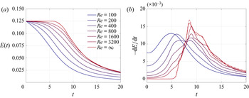
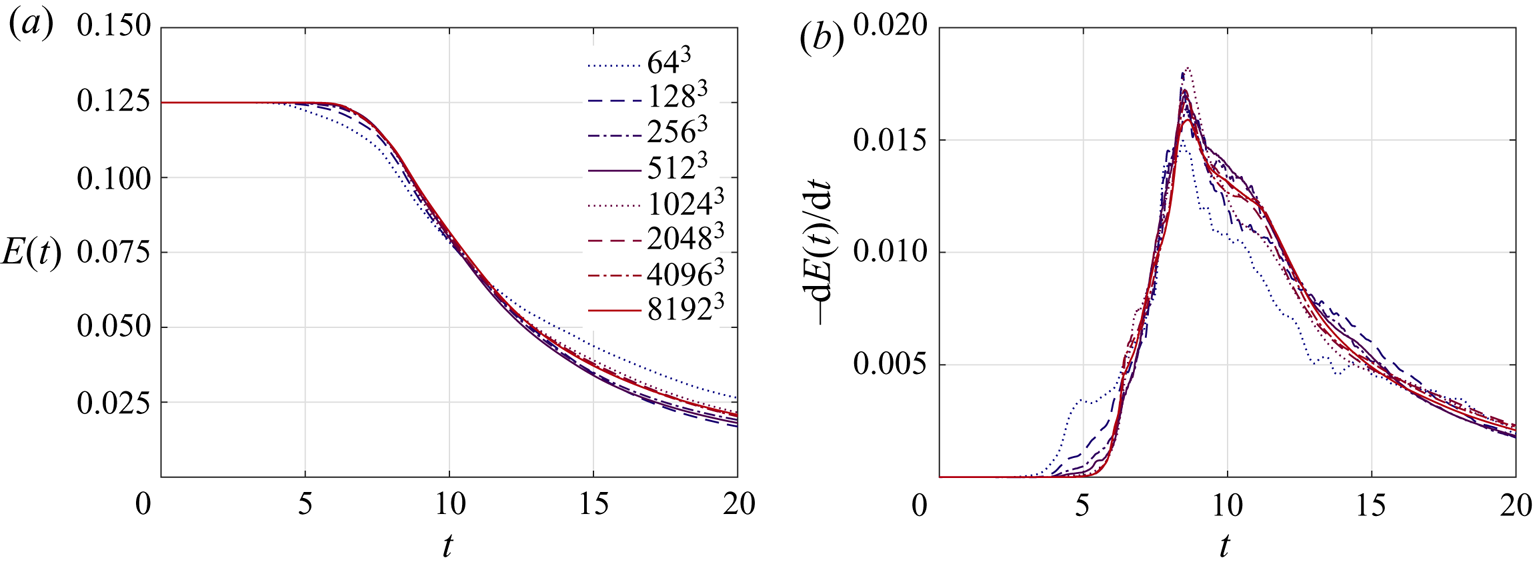
 $\nu \rightarrow 0$. This argument is summarised in figure 1, which shows results for viscous and inviscid simulations of the Taylor–Green vortex obtained with the present discretisation approach. For each Reynolds number, results are shown for two resolutions of the numerical discretisation approach to judge whether the results are mesh-independent. We achieve grid-converged results for all finite Reynolds numbers shown in figure 1. In the inviscid limit, the temporal evolution of the kinetic energy is almost indistinguishable for the two finest resolutions, while small differences in the energy dissipation rate are still visible between the two resolutions
 $4096^3$ and
 $8192^3$ at later times around the dissipation maximum and beyond. However, the onset of dissipation around
 $t\approx 6$ appears to be grid-converged also for this challenging inviscid simulation. These results are consistent with grid-convergence to a dissipative solution of the incompressible Euler equations for the three-dimensional Taylor–Green problem. Figure 1 therefore summarises the main result of the present work.
Temporal evolution of kinetic energy (a) and kinetic energy dissipation rate (b) for the three-dimensional Taylor–Green vortex problem for increasing Reynolds numbers of  $Re=100,200,400,800,1600,3200,\infty$. For each
 $Re$, results are shown for two mesh resolutions (fine mesh as solid line, coarse mesh as dashed-dotted line). The effective resolutions (see § 3 for a definition) are
 $64^3, 128^3$ for
 $Re=100$,
 $128^3, 256^3$ for
 $Re=200, 400$,
 $256^3, 512^3$ for
 $Re=800$,
 $1024^3, 2048^3$ for
 $Re=1600$,
 $2048^3, 4096^3$ for
 $Re=3200$, and
 $4096^3, 8192^3$ for
 $Re=\infty$. The results suggest that the kinetic energy reduces to a value as low as approximately
 $0.02$ at time
 $t=20$ for large Reynolds numbers, and that a similar amount of energy dissipation also takes place in the inviscid limit.

While the accumulation of energy in small scales in case of energy-preserving schemes is unphysical, it can be exploited under certain circumstances in order to gain insights into the physical dissipation behaviour. In Cichowlas et al. (Reference Cichowlas, Bonaïti, Debbasch and Brachet2005), an effective dissipation is estimated from the small-scale thermalised energy of energy-conserving, spectrally truncated Euler simulations, and it is found that the large-scale Euler dynamics are similar to high-Reynolds-number Navier–Stokes dynamics. Although the underlying numerical methods in that work are different from those of the present study (the energy dissipation rate is derived by a postprocessing of results in Cichowlas et al. (Reference Cichowlas, Bonaïti, Debbasch and Brachet2005), whereas it is simulated directly in the present work), there are interesting parallels. The onset of dissipation around  $t=5 - 6$ and the dissipation maximum around
 $t = 8 - 9$ appear to be very similar to the present results, so that the two studies can be seen to complement and verify each other. From this perspective, the study by Cichowlas et al. (Reference Cichowlas, Bonaïti, Debbasch and Brachet2005) supports the main conclusions of our work.
Instead of considering a two-parameter limit problem  $h \to 0, \nu \to 0$ as illustrated in figure 1, the remainder of this work focuses on the one-parameter limit
 $h \to 0$ for the inviscid limit
 $\nu = 0$. Let us explain this decision in more detail. A two-parameter study
 $h \to 0, \nu \to 0$ would technically not be realisable due to the large amount of computational costs required for such simulations: already for moderate Reynolds numbers of
 $Re={O}(10^4)$, as considered for example in Arndt et al. (Reference Arndt, Fehn, Kanschat, Kormann, Kronbichler, Munch, Wall and Witte2020) and Lamballais et al. (Reference Lamballais, Dairay, Laizet and Vassilicos2019), the spatial resolutions required for grid-convergence are comparable to the highest-resolution simulations that we are able to realise in the present work for the inviscid limit. These highest-resolution simulations require computational costs of tens of millions of CPUh in the present study, despite the fact that we use a highly efficient implementation that is well optimised for the hardware under consideration. With the goal of realising spatial resolutions as high as those shown in the present study, computational costs would allow us to consider only a single finite Reynolds number beyond what is shown in figure 1, which explains why we immediately address the inviscid limit
 $\nu = 0$.
1.5. Outline
The rest of this article is organised as follows. We describe the mathematical model of the incompressible Navier–Stokes or Euler equations and its numerical discretisation in space and time in § 2. Section 3 shows results for the one-dimensional Burgers equation with formation of a shock, a two-dimensional shear layer problem with a numerical investigation of the kinetic energy dissipation in the limit  $\nu \rightarrow 0$, and finally the three-dimensional Taylor–Green vortex problem that has been suspected to exhibit finite-time singularities in the inviscid limit. In § 4, we summarise our results, draw conclusions and raise questions based on the present observations.
2. Numerical methods
We seek numerical solutions to the incompressible Euler equations solved on a domain  $\varOmega \subset \mathbb {R}^d$ in
 $d=2,3$ space dimensions. These have their origin in the equations for viscous fluids with kinematic viscosity
 $\nu$ described by the incompressible Navier–Stokes equations
 $$\begin{gather} \frac{\partial \boldsymbol{u}}{\partial t} + \boldsymbol{\nabla} \boldsymbol{\cdot} (\boldsymbol{u} \otimes \boldsymbol{u}) - \nu \nabla^2 \boldsymbol{u} + \boldsymbol{\nabla} p = \boldsymbol{0}, \end{gather}$$
 $$\begin{gather}\boldsymbol{\nabla}\boldsymbol{\cdot} \boldsymbol{u} = 0 , \end{gather}$$
where  $\boldsymbol {u}$ denotes the
 $d$-dimensional velocity vector and
 $p$ the kinematic pressure. The Euler equations are recovered by setting
 $\nu =0$. This system of partial differential equations does not extend to
 $d=1$ in a meaningful way, since the incompressibility constraint
 $\partial u /\partial x = 0$ would imply
 $u = \text {const}$. (However, the one-dimensional Burgers equation serves as a simplified mathematical model for more complex higher-dimensional problems. While results for the inviscid Burgers equation are presented in § 3, this section deals with discretisations of the incompressible Navier–Stokes equations for
 $d=2,3$.) Let us note that the temporal and spatial discretisation schemes discussed below are generic and hold for both two- and three-dimensional problems, but that there are major differences in terms of the flow physics and the mechanisms that make up the nature of turbulence, such as the energy transfer to small scales according to a turbulence cascade in three dimensions (Onsager Reference Onsager1949). This fundamentally different behaviour is attributed to the vortex-stretching term in the vorticity form of the Euler equations (Gibbon Reference Gibbon2008),
 \begin{equation} \frac{\mathrm{D}\boldsymbol{\omega}}{\mathrm{D}t} = \left(\boldsymbol{\omega}\boldsymbol{\cdot}\boldsymbol{\nabla}\right) \boldsymbol{u}, \end{equation}
where the vortex-stretching term on the right-hand side vanishes in two dimensions since the vorticity  $\boldsymbol {\omega }$ is perpendicular to the velocity
 $\boldsymbol {u}$ in that case.
The following two subsections detail the temporal and spatial discretisation of the incompressible Navier–Stokes equations (2.1) and (2.2). Discretisation in time is based on projection methods that solve for velocity and pressure unknowns in different sub-steps of a time step. Discretisation in space is based on high-order DG methods with suitable stabilisation techniques that render the method robust for under-resolved, high-Reynolds-number flows.
2.1. Temporal discretisation – high-order projection method
Discretisation in time is based on projection methods which aim at obtaining computationally efficient incompressible flow solvers by decoupling the velocity and pressure unknowns (Karniadakis & Sherwin Reference Karniadakis and Sherwin2005). A convection–diffusion-type problem is solved for the velocity and a Poisson equation for the pressure, with a subsequent projection of the velocity onto the space of solenoidal vector fields according to the Helmholtz decomposition. We use the high-order dual splitting scheme proposed in Karniadakis, Israeli & Orszag (Reference Karniadakis, Israeli and Orszag1991), which consists of the following four sub-steps:
 $$\begin{gather} \frac{\displaystyle\gamma_0^n\hat{\boldsymbol{u}}-\sum_{i=0}^{J-1}\alpha_i^n\boldsymbol{u}^{n-i}}{\Delta t_n} ={-} \sum_{i=0}^{J-1}\beta_i^n \boldsymbol{\nabla} \boldsymbol{\cdot} {(\boldsymbol{u}^{n-i} \otimes \boldsymbol{u}^{n-i})}, \end{gather}$$
 $$\begin{gather}-\nabla^2 p^{n+1} ={-}\frac{\gamma_0^n }{\Delta t_n}\boldsymbol{\nabla} \boldsymbol{\cdot} {\hat{\boldsymbol{u}}}, \end{gather}$$
 $$\begin{gather}\hat{\hat{\boldsymbol{u}}} = \hat{\boldsymbol{u}} - \frac{\Delta t_n}{\gamma_0^n} \boldsymbol{\nabla}{p^{n+1}}, \end{gather}$$
 $$\begin{gather}\frac{\gamma_0^n}{\Delta t_n} \boldsymbol{u}^{n+1} - \nu \nabla^2 \boldsymbol{u}^{n+1} = \frac{\gamma_0^n}{\Delta t_n}\hat{\hat{\boldsymbol{u}}}, \end{gather}$$
where  $n$ denotes the current time step, in which the equations are integrated from time
 $t_n$ to time
 $t_{n+1} = t_n + \Delta t_n$. The temporal discretisation is based on a backward differentiation formula of order
 $J$ with coefficients
 $\gamma _0^n$ and
 $\alpha _i^n,\ i=0,\ldots,J-1$. In the first sub-step (2.4), the convective term is treated explicitly in time by using a high-order extrapolation scheme of order
 $J$ with coefficients
 $\beta _i^n, i=0, \ldots ,J-1$. In the next two sub-steps, a pressure Poisson equation (2.5) is solved and a divergence-free velocity is obtained in the projection step (2.6). Finally, the viscous term is taken into account in the last sub-step (2.7), which can be omitted in the case of the Euler equations,
 $\boldsymbol {u}^{n+1} = \hat {\hat {\boldsymbol {u}}}$. The explicit treatment of the convective term implies a restriction of the time step size according to the Courant–Friedrichs–Lewy (CFL) condition. For reasons of computational efficiency, we use adaptive time stepping with variable time step sizes
 $\Delta t_n$, readjusting the time step size after each time step in such a way as to maximise the time step size and operate close to the CFL stability limit. We introduce the CFL condition below since it also depends on the spatial discretisation scheme. A second-order accurate time integration scheme with
 $J=2$ is used in the present work.
2.2. Spatial discretisation – high-order discontinuous Galerkin method
A key element of the present study is the use of a novel high-order DG discretisation for incompressible flows. This discretisation approach has been developed recently and is documented in a series of publications (Fehn, Wall & Kronbichler Reference Fehn, Wall and Kronbichler2017; Krank et al. Reference Krank, Fehn, Wall and Kronbichler2017; Fehn, Wall & Kronbichler Reference Fehn, Wall and Kronbichler2018b; Fehn et al. Reference Fehn, Kronbichler, Lehrenfeld, Lube and Schroeder2019), with a focus on the stability of projection methods in Fehn et al. (Reference Fehn, Wall and Kronbichler2017), and a focus on the stability and dissipation characteristics of DG discretisations for under-resolved turbulence in Fehn et al. (Reference Fehn, Wall and Kronbichler2018b, Reference Fehn, Kronbichler, Lehrenfeld, Lube and Schroeder2019). Of particular importance are the inbuilt dissipation mechanisms of DG methods acting on the finest resolved scales of the flow. In order to investigate the phenomenon of anomalous energy dissipation, we consider it a prerequisite to use a discretisation scheme that provides the flexibility to find both dissipative and non-dissipative solutions. Let us point out that all simulations shown in this work are performed as direct numerical simulations, i.e. without any form of explicit turbulence model or numerical viscosity. More precisely, upwind-type numerical fluxes represent the main dissipation mechanism of the present scheme; see also Ainsworth (Reference Ainsworth2004) for a general dispersion and dissipation analysis and distribution of dissipation among the resolved scales. Note that the  $H(\text {div})$-stabilisation presented below also contributes with a certain amount of dissipation. For reasons of brevity and to focus on the main aspects, we avoid technical aspects related to the imposition of boundary conditions in the following, but refer to the original publications.
We assume a computational domain  $\varOmega _h= \bigcup _{e=1}^{N_{{el}}} \varOmega _{e} \in \mathbb {R}^d$ consisting of conforming quadrilateral or hexahedral elements
 $\varOmega _e$,
 $e=1,\ldots, N_{{el}}$. A common abstraction of finite element methods is to define a mapping
 $\boldsymbol {x}^e(\boldsymbol {\xi })$ from a reference element
 $\tilde {\varOmega }_e = [0,1]^d$ with Cartesian coordinates
 $\boldsymbol {\xi }$ to element
 $\varOmega _e$ in physical space with coordinates
 $\boldsymbol {x}$, and approximate the solution within each element by polynomials defined in reference coordinates. Here, the numerical solution in
 $d=2,3$ is represented by a tensor product of one-dimensional Lagrange polynomials with a Legendre–Gauss–Lobatto point distribution, and is allowed to exhibit discontinuities between elements in an
 $L^2$-conforming sense. The spaces of shape functions are then given as
 \begin{align} \mathcal{V}^{u}_{h} &= \lbrace\boldsymbol{u}_h\in [L^2(\varOmega_h)]^d: \boldsymbol{u}_h\left(\boldsymbol{x}^e(\boldsymbol{\xi})\right)\vert_{\varOmega_{e}}= \tilde{\boldsymbol{u}}_h^e(\boldsymbol{\xi})\vert_{\tilde{\varOmega}_{e}}\in \mathcal{V}^{u}_{h,e}=[\mathcal{Q}_{k}(\tilde{\varOmega}_{e})]^d,\nonumber\\ &\quad \vphantom{\left[L^2(\varOmega_h)\right]^d} \forall\ e=1,\ldots,N_{{el}}\rbrace, \end{align}
 \begin{align} \mathcal{V}^{p}_{h} &= \lbrace p_h\in L^2(\varOmega_h): p_h(\boldsymbol{x}^e(\boldsymbol{\xi}))\vert_{\varOmega_{e}} = \tilde{p}_h^e(\boldsymbol{\xi})\vert_{\tilde{\varOmega}_{e}}\in \mathcal{V}^{p}_{h,e}=\mathcal{Q}_{k-1}(\tilde{\varOmega}_{e}), \nonumber\\ &\quad \vphantom{\left(\boldsymbol{x}^e(\boldsymbol{\xi})\right)\vert_{\varOmega_{e}} = \tilde{p}_h^e(\boldsymbol{\xi})\vert_{\tilde{\varOmega}_{e}}\in \mathcal{V}^{p}_{h,e}} \forall\ e=1,\ldots,N_{{el}}\rbrace. \end{align}
Here,  $\mathcal {Q}_{k}$ denotes the space of tensor-product polynomials of degree
 $k$, and we highlight the ambiguity in notation related to the spatial wavenumber
 $k$ in the context of energy spectra. The polynomial degree of the velocity shape functions is
 $k$, while it is
 $k-1$ for the pressure for reasons of inf–sup stability. In this work, we only consider problems with Cartesian meshes so that the mapping
 $\boldsymbol {x}^e(\boldsymbol {\xi })$ is an affine transformation. At the interface between two elements
 $e^-$ and
 $e^+$, the numerical solution is not unique, and we use the superscripts
 $-$ and
 $+$ to denote the solution from the two sides of an interface. When referring to the element
 $e$, we denote interior information by
 $-$, and the outward-pointing unit normal vector by
 $\boldsymbol {n}=\boldsymbol {n}^-$. To define numerical fluxes, we introduce the average operator
 $\{\!\{u\}\!\}=(u^- + u^+)/2$ and the jump operator
 $\left[\kern-0.15em\left[ {u} \right]\kern-0.15em\right] =u^- \otimes \boldsymbol {n}^- + u^+ \otimes \boldsymbol {n}^+$, where
 $\boldsymbol {n}^+ = - \boldsymbol {n}^-$. We apply the usual abbreviations of integrals,
 $\left ( {v},{u} \right )_{\varOmega _{e}} = \int _{\varOmega _e} v \odot u\, \mathrm {d}\varOmega$ for volume integrals and
 $\left ( {v},{u} \right )_{\partial \varOmega _{e}} = \int _{\partial \varOmega _e} v \odot u \,\mathrm {d} \varGamma$ for surface integrals with
 $\odot$ denoting an inner product. We now state the weak formulation for all sub-steps of the projection scheme. We obtain the numerical solutions
 $\hat {\boldsymbol {u}}_h,\hat {\hat {\boldsymbol {u}}}_h, \hat {\hat {\hat {\boldsymbol {u}}}}_h ,\boldsymbol {u}_h^{n+1}\in \mathcal {V}^u_h$ and
 $p_h^{n+1}\in \mathcal {V}^p_h$ by testing with all test functions
 $\boldsymbol {v}_h \in \mathcal {V}^{u}_{h,e}$,
 $q_h \in \mathcal {V}^{p}_{h,e}$ for all elements
 $e=1,\ldots,N_{{el}}$.
In the first step, the convective term is discretised by the local Lax–Friedrichs flux
 \begin{align} & \left( {\boldsymbol{v}_h},{\frac{\gamma_0^n \hat{\boldsymbol{u}}_h-\sum_{i=0}^{J-1}\alpha_i^n\boldsymbol{u}^{n-i}_h}{\Delta t_n}} \right)_{\varOmega_{e}} ={-} \sum_{i=0}^{J-1} \beta_i^n \left(- \left( {\boldsymbol{\nabla}{\boldsymbol{v}_h}},{\left(\boldsymbol{u}_h \otimes \boldsymbol{u}_h\right)^{n-i}} \right)_{\varOmega_{e}} \vphantom{\left(\{\!\{\boldsymbol{u}_h \otimes \boldsymbol{u}_h\}\!\} +\frac{\varLambda}{2}\left[\kern-0.15em\left[ {\boldsymbol{u}_h} \right]\kern-0.15em\right] \right)^{n-i}}\right.\nonumber\\ &\quad \left.+ \left( {\boldsymbol{v}_h},{\left(\{\!\{\boldsymbol{u}_h \otimes \boldsymbol{u}_h\}\!\} + \frac{\varLambda}{2}\left[\kern-0.15em\left[ {\boldsymbol{u}_h} \right]\kern-0.15em\right] \right)^{n-i}\boldsymbol{\cdot} \boldsymbol{n}} \right)_{\partial\varOmega_{e}} \right), \end{align}
where the stabilisation parameter is chosen as  $\varLambda = \max ( \vert \boldsymbol {u}_h^{-} \boldsymbol {\cdot } \boldsymbol {n}\vert, \vert \boldsymbol {u}_h^{+} \boldsymbol {\cdot } \boldsymbol {n}\vert )$. The pressure Poisson operator is discretised by the symmetric interior penalty Galerkin (SIPG) method
 \begin{align} & ({\boldsymbol{\nabla}{q_h}},{\boldsymbol{\nabla}{p^{n+1}_h}})_{\varOmega_{e}} - \left(
{\boldsymbol{\nabla}{q_h}},{\frac{1}{2}\left[\kern-0.15em\left[ {p^{n+1}_h} \right]\kern-0.15em\right] } \right)_{\partial\varOmega_{e}} -
({q_h},{\{\!\{\boldsymbol{\nabla}{p^{n+1}_h}\}\!\}\boldsymbol{\cdot}\boldsymbol{n}})_{\partial\varOmega_{e}} \nonumber\\
&\quad + ( {q_h},{\tau\left[\kern-0.15em\left[ {p^{n+1}_h} \right]\kern-0.15em\right]
\boldsymbol{\cdot}\boldsymbol{n}}
)_{\partial\varOmega_{e}} ={-} \frac{\gamma_0^n}{\Delta
t_n} ( - ( {\boldsymbol{\nabla}{q_h}},{\hat{\boldsymbol{u}}_h} )_{\varOmega_{e}} + (
{q_h},{\{\!\{\hat{\boldsymbol{u}}_h\}\!\}\boldsymbol{\cdot}\boldsymbol{n}})_{\partial\varOmega_{e}}),
\end{align}
where a central flux is used for the velocity divergence operator on the right-hand side of the pressure Poisson equation. A central flux is also used for the pressure gradient term in the projection step
 \begin{equation} (
{\boldsymbol{v}_h},{\hat{\hat{\boldsymbol{u}}}_h}
)_{\varOmega_{e}} = (
{\boldsymbol{v}_h},{\hat{\boldsymbol{u}}_h}
)_{\varOmega_{e}} - \frac{\Delta t_n}{\gamma_0^n}
( - ( {\boldsymbol{\nabla} \boldsymbol{\cdot}
{\boldsymbol{v}_h}},{p^{n+1}_h})_{\varOmega_{e}} +
( {\boldsymbol{v}_h},{\{\!\{p^{n+1}_h\}\!\}\boldsymbol{n}}
)_{\partial\varOmega_{e}}).
\end{equation}
The viscous term is also discretised by the SIPG method,
 \begin{array}{l} \textrm{ }{\left( {{\boldsymbol{v}_h},\frac{{\gamma _0^n}}{{{\Delta }{t_n}}}{{\hat {\hat {\hat {\boldsymbol{u}}}}}_h}} \right)_{{{\Omega }_e}}} + \textrm{ }{\left( {\nabla {\boldsymbol{v}_h},\nu \nabla {{\hat {\hat {\hat {\boldsymbol{u}}}}}_h}} \right)_{{{\Omega }_e}}} - \textrm{ }{\left( {\nabla {\boldsymbol{v}_h},\frac{\nu }{2}\left[\kern-0.15em\left[{{\hat {\hat {\hat {\boldsymbol{u}}}}}_h}\right]\kern-0.15em\right]} \right)_{\partial {{\Omega }_e}}}\\ \quad - \textrm{ }{\left( {{\boldsymbol{v}_h},\nu \textrm{ \{ \{ }\nabla {{\hat {\hat {\hat {\boldsymbol{u}}}}}_h}\} \} \cdot {\boldsymbol{n}}} \right)_{\partial {{\Omega }_e}}} + \textrm{ }{\left( {{\boldsymbol{v}_h},\nu \tau \left[\kern-0.15em\left[{{\hat {\hat {\hat {\boldsymbol{u}}}}}_h}\right]\kern-0.15em\right] \cdot {\boldsymbol{n}}} \right)_{\partial {{\Omega }_e}}} = \textrm{ }{\left( {{\boldsymbol{v}_h},\frac{{\gamma _0^n}}{{{\Delta }{t_n}}}{{\hat {\hat {\boldsymbol{u}}}}_h}} \right)_{{{\Omega }_e}}}, \end{array}
while this step is skipped,  $\hat {\hat {\hat {\boldsymbol {u}}}}_h = \hat {\hat {\boldsymbol {u}}}_h$, in the inviscid limit when solving the incompressible Euler equations. In a final postprocessing step, consistent divergence and continuity penalty terms are applied to weakly enforce the incompressibility constraint and normal continuity of the velocity field (Fehn et al. Reference Fehn, Wall and Kronbichler2018b, Reference Fehn, Heinz, Wall and Kronbichler2021):
 \begin{align} & (
{\boldsymbol{v}_h},{\boldsymbol{u}_h^{n+1}}
)_{\varOmega_{e}} + ( {\boldsymbol{\nabla}
\boldsymbol{\cdot}
{\boldsymbol{v}_h}},{\tau_{D}\boldsymbol{\nabla}
\boldsymbol{\cdot} {\boldsymbol{u}_h^{n+1}}}
)_{\varOmega_{e}} \Delta t_n \nonumber\\ &\quad +
( {\boldsymbol{v}_h\boldsymbol{\cdot}
\boldsymbol{n}},{\tau_{C}
(\boldsymbol{u}_h^{-} -
\boldsymbol{u}_h^{+})^{n+1}\boldsymbol{\cdot}
\boldsymbol{n}} )_{\partial\varOmega_{e}} \Delta t_n =
(
{\boldsymbol{v}_h},{\hat{\hat{\hat{\boldsymbol{u}}}}_h} )_{\varOmega_{e}} . \end{align}
The above postprocessing step is specifically related to the type of spatial discretisation used in this work, i.e. the  $L^2$-conforming DG method, and disappears in the continuous case. It was found that the divergence and normal-continuity penalty terms are crucial in terms of mass conservation and energy stability in order to obtain a method that is robust for large Reynolds numbers and coarse spatial resolutions, and we refer to Fehn et al. (Reference Fehn, Wall and Kronbichler2018b, Reference Fehn, Kronbichler, Lehrenfeld, Lube and Schroeder2019) for detailed numerical justification and validation of this approach. In this context, we note that alternatives to this stabilised approach exist, e.g. by using tailored finite element function spaces. For example, function spaces can be used that result in an
 $H(\text {div})$-conforming (normal-continuous) velocity field and that is divergence-free in every point of the computational domain. The present
 $L^2$-conforming approach does not fulfil these two properties exactly, but in a weak finite element sense. Definitions of the penalty parameters
 $\tau, \tau _{{D}}, \tau _{{C}}$ are given in Fehn et al. (Reference Fehn, Wall and Kronbichler2018b), where the default penalty factor
 $\zeta =1$ is used in the present work unless specified otherwise. In terms of the occurrence of finite-time singularities and anomalous energy dissipation, the present work makes use of the argument that – due to the weighted residual formulation – the present discretisation can be applied to problems which lack regularity and for which the differential form of the equations is no longer an appropriate description. With respect to the implementation of the method, integrals in the weak form are evaluated by means of Gaussian quadrature, with consistent integration according to the
 $3/2$ rule for the nonlinear convective term (also known as polynomial dealiasing). Since we consider uniform Cartesian meshes (with elements of size
 $h$ in all coordinate directions) in the present work, integrals are calculated exactly.
To obtain the size of the next time step within the adaptive time stepping scheme, we use the following local CFL condition evaluated at all quadrature points  $q$ of element
 $e$:
 \begin{equation} \Delta t = \min_{e=1,\ldots,N_{{el}}} \left(\min_{q}\frac{Cr}{k^{1.5}} \left.\frac{h}{\Vert \boldsymbol{u}_h \Vert }\right\vert_{q,e} \right).\end{equation}
where we ensure stability of the time integration scheme by selecting a Courant number  ${Cr} < {Cr}_{{crit}}$. Note that – due to the CFL condition – an increase in spatial resolution by reducing
 $h$ or increasing
 $k$ automatically implies an increase in temporal resolution through a reduced time step size.
The present incompressible flow solver is implemented in C++ and forms a core module of the ExaDG (High-Order Discontinuous Galerkin for the Exa-Scale) software, which is publicly available on github (see https://github.com/exadg/exadg). The ExaDG software primarily makes use of the open-source finite element library deal.II (Alzetta et al. Reference Alzetta2018; Arndt et al. Reference Arndt, Bangerth, Davydov, Heister, Heltai, Kronbichler, Maier, Pelteret, Turcksin and Wells2021). The computational efficiency of the present discretisation methods in terms of fast implementations and fast iterative solvers is discussed in Fehn, Wall & Kronbichler (Reference Fehn, Wall and Kronbichler2018a), Fehn et al. (Reference Fehn, Munch, Wall and Kronbichler2020), Kronbichler & Kormann (Reference Kronbichler and Kormann2019) and Arndt et al. (Reference Arndt, Fehn, Kanschat, Kormann, Kronbichler, Munch, Wall and Witte2020).
3. Results
This section presents numerical results for three test cases in  $d=1$,
 $d=2$ and
 $d=3$ space dimensions. The one-dimensional problem is the well-known inviscid Burgers equation developing a singularity in finite time for appropriate initial conditions. The two-dimensional example is a shear layer roll-up problem. The particular example used for the
 $d=2$ investigations is not of primary importance, as it is known theoretically that regularity is expected for two-dimensional Euler flows when starting from regular initial data. Instead, the aim of these one- and two-dimensional examples is to investigate to what extent the numerical discretisation scheme is able to mimic physical behaviour with potentially singular solutions. Having validated the numerical method for these well-understood problems, we apply it to the three-dimensional inviscid Taylor–Green problem, for which the physical understanding in terms of the occurrence of finite-time singularities and the related aspect of anomalous energy dissipation is speculative at present. As further preparation, we summarise the quantities of interest in the following subsection.
3.1. Quantities of interest
Since turbulent flows in three space dimensions are our primary interest, we restrict the discussion in this subsection to the three-dimensional case, implying extensions of certain relations to one- and two-dimensional problems only where possible. Of primary importance for the present study is the temporal evolution of the kinetic energy
 \begin{equation} E(t) = \frac{1}{V_{\varOmega}} \int_{\varOmega} \frac{1}{2} \boldsymbol{u}(\boldsymbol{x},t) \boldsymbol{\cdot} \boldsymbol{u}(\boldsymbol{x},t)\,\mathrm{d}\varOmega \end{equation}
and its dissipation rate  $\mathrm {d} E / \mathrm {d} t$. The kinetic energy is normalised by the volume
 $V_{\varOmega } = \int _{\varOmega } 1 \,\mathrm {d}\varOmega$ of the computational domain. The integrals are evaluated numerically by means of Gaussian quadrature, with
 $k+1$ quadrature points in each coordinate direction. The time derivative used to obtain the dissipation rate is computed numerically from the kinetic energy at discrete instants of time via a second-order finite difference formula for variable time step sizes with first-order approximations at the end points. If anomalous dissipation (
 $\mathrm {d} E / \mathrm {d} t < 0$) occurs, the temporal evolution of the enstrophy
 $\mathcal {E}$,
 \begin{equation} \mathcal{E}(t) = \frac{1}{V_{\varOmega}} \int_{\varOmega} \frac{1}{2} \boldsymbol{\omega}(\boldsymbol{x},t) \boldsymbol{\cdot} \boldsymbol{\omega}(\boldsymbol{x},t)\,\mathrm{d}\varOmega, \end{equation}
is expected to exhibit a singularity  $\mathcal {E} \rightarrow \infty$ in finite time. Integrals are computed by Gaussian quadrature, which is exact down to round-off errors due to polynomial integrands and Cartesian meshes. A related local quantity is the maximum vorticity
 \begin{equation} \Vert \boldsymbol{\omega} \Vert_{\infty} (t), \end{equation}
where we take the maximum over all quadrature points over all elements in the discrete case and monitor its evolution over time, with a view to detecting potentially singular behaviour in finite time. Although the maximum vorticity will remain finite for every numerical simulation of finite resolution, a mesh refinement study may give hints about the expected behaviour if the resolution is further increased. Finally, we consider kinetic energy spectra by transformation into wavenumber space  $\boldsymbol {k}$ (Cichowlas & Brachet Reference Cichowlas and Brachet2005; Bustamante & Brachet Reference Bustamante and Brachet2012):
 \begin{align} E(k, t) = \frac{1}{2} \lim_{\Delta k \rightarrow 0} \frac{\displaystyle\int_{\Vert \boldsymbol{k} \Vert=k}^{\Vert \boldsymbol{k} \Vert=k+\Delta k} \Vert \hat{\boldsymbol{u}}(\boldsymbol{k},t)\Vert^2 \mathrm{d} \boldsymbol{k}}{\Delta k}\hspace{0,5cm} \overset{\text{DFT}}{\approx} \sum_{\substack{\boldsymbol{k} \in \mathbb{Z}^3 \\ k-\frac{1}{2} \leq \Vert \boldsymbol{k} \Vert < k+\frac{1}{2}}} \frac{1}{2} \Vert \hat{\boldsymbol{u}}_{\mathrm{DFT}}(\boldsymbol{k},t)\Vert^2, \end{align}
where  $\hat {\boldsymbol {u}}(\boldsymbol {k},t)$ denotes the Fourier transform of the velocity, which only exists at discrete wavenumber vectors
 $\boldsymbol {k}$ in case of a discrete Fourier transformation (DFT) obtained from sampled data of a discrete velocity field. The solution is first interpolated onto
 $N$ equidistant points per element and per coordinate direction to which the discrete Fourier transformation is applied, using the library FFTW (Frigo & Johnson Reference Frigo and Johnson2005) in the present work. (The number of sampling points is chosen as
 $N=k+1$ in the present work, i.e. equal to the number of nodal points of the DG discretisation, where
 $k$ is the polynomial degree of the shape functions and should not be confused with the wavenumber
 $k$ typically used in the context of energy spectra. The equidistant interpolation points all lie within the element, away from the boundaries where the solution is discontinuous. If interpolation points on the boundary are used, one typically takes the average of the solutions from neighbouring elements.) Note that considering
 $E(k,t)$ as a function of a scalar wavenumber
 $k$ as well as the summation over spheres of radius
 $k$ introduces the assumptions of homogeneity and isotropy. In case of anomalous energy dissipation, the enstrophy is expected to become infinite. Hence, exploiting the relation
 $\mathcal {E}(k,t) = k^2 E(k,t)$ between the enstrophy and energy spectra and further assuming a power law behaviour for the kinetic energy spectrum of the form
 $E(k,t) = C(t) k^{-n (t)}$, a singularity at time
 $t=t_*$ with
 $\mathcal {E}(t_*) = \int _0^{\infty } \mathcal {E}(k,t_*) \,\mathrm {d}k = \infty$ would correspond to a decay with slope
 $n(t_*)=3$ in the energy spectrum; see also Orlandi (Reference Orlandi2009) and Orlandi et al. (Reference Orlandi, Pirozzoli and Carnevale2012). We use this criterion as further validation of the results in case other quantities give hints of potentially singular behaviour. Apart from that, energy spectra are typically investigated to assess the well-known
 $k^{-5/3}$ Kolmogorov spectrum for fully-developed, homogeneous isotropic turbulence. We apply this property to investigate whether the numerical results match expected physical behaviour obtained from classical cascade pictures in case of inviscid flows and beyond the time of potential singularities,
 $t > t_*$.
3.2. One-dimensional inviscid Burgers equations
We begin by studying the one-dimensional inviscid Burgers equation (Burgers Reference Burgers1948)
 \begin{equation} \frac{\partial u}{\partial t} + \frac{\partial }{\partial x} \frac{u^2}{2} = 0, \end{equation}
as a simplified model for the incompressible Euler equations. It is well known that this equation develops singularities in finite time; see for example Sulem et al. (Reference Sulem, Sulem and Frisch1983) and Dubrulle (Reference Dubrulle2019). Previous works demonstrate that the use of energy-conserving discretisation schemes leads to thermalisation for this type of problem; see for example Ray et al. (Reference Ray, Frisch, Nazarenko and Matsumoto2011) and Murugan et al. (Reference Murugan, Frisch, Nazarenko, Besse and Ray2020). It is therefore particularly interesting to study the behaviour of a discretisation scheme for this simplified problem first. The spatial discretisation is based on a DG scheme very similar to the one described in § 2 for the two- and three-dimensional cases; i.e. the convective term is discretised with a local Lax–Friedrichs flux. Gaussian quadrature with a  $3/2$-overintegration rule is used as in the higher-dimensional case, due to the quadratic nonlinearity of the convective term, but we intentionally take no additional measure, such as limiting, filtering, or other Riemann fluxes, to specifically address the jump that forms in the solution. We also emphasise that no artificial viscosity approach is used to deal with the singularity. For time integration, the classical explicit fourth-order Runge–Kutta method is used with a Courant number of
 ${Cr}=0.4$.
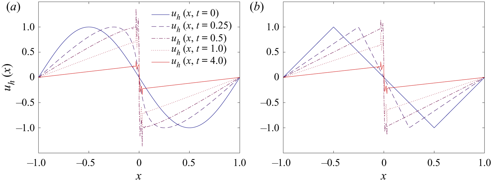
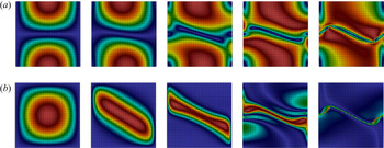
Figure 2 shows the numerical solution  $u_h(x)$ at various instants of time and the formation of a shock. The problem is solved on the domain
 $\varOmega = [-1, 1]$ with Dirichlet boundary conditions prescribed at both boundary points of the one-dimensional domain. An equidistant grid with
 $2^l$ elements is used, where
 $l$ denotes the level of refinement. For polynomial approximations of degree
 $k$, the effective resolution becomes
 $(k+1)2^l$. For illustration, we select two different initial solutions: a sine function,
 $u_h(x, t=0) = - \sin ({\rm \pi} x)$, and a hat function,
 $u_h(x, t=0) = - 2 \vert x + 0.5 \vert + 1$ for
 $x < 0$ and
 $u_h(x, t=0) = 2 \vert x - 0.5 \vert -1$ for
 $x \geq 0$. Due to the chosen initial conditions with
 $u>0$ for
 $x<0$ and vice versa, the solution piles up in the middle of the domain and a singularity (
 $\partial u /\partial x \rightarrow \infty$) forms at
 $x=0$ in both cases. The oscillating behaviour of the numerical solution around the singularity could be improved by the advanced discretisation techniques mentioned above. From the results shown in figure 2 it is plausible that the kinetic energy is conserved until the formation of the shock and that energy will be dissipated at later times. For the hat function chosen as the initial condition, it is straightforward to derive an analytical expression for the temporal evolution of the kinetic energy as well as its dissipation rate, which is why we consider this setup in more detail in the following. According to the method of characteristics it follows that the shock forms at time
 $t_*=0.5$. From that time on, the solution can be written as
 \begin{equation} u(x,t) = f(t) \left(x - \text{sign} (x) \right), \end{equation}
where  $\text {sign} (x)$ takes values of
 $\pm 1$ depending on the sign of the argument. The temporal evolution part
 $f(t)$, which describes the absolute value of
 $u$ taken to the left and right of the origin of the coordinate system at
 $x=0$, can be obtained from the following consideration:
 \begin{equation} f(t + \mathrm{d}t) = f(t) - \underbrace{\left.\frac{\partial u (x,t)}{\partial x}\right\vert_{x=0^-}}_{{=}f(t)} \underbrace{\mathrm{d}x}_{\substack{= u(x=0^-,t)\,\mathrm{d}t \\ = f(t)\,\mathrm{d}t}} = f(t) \left(1 - f(t)\,\mathrm{d}t\right); \end{equation}
i.e. the solution at  $x=0^-$ at time
 $t+\mathrm {d}t$ equals the solution at position
 $-\mathrm {d}\kern0.06em x = -u(x=0^-,t)\,\mathrm {d}t$ at time
 $t$. Separation of variables and integration yields the result
 $f(t) = 1 /(t+t_*)$. The kinetic energy
 $E(t) = \int _{\varOmega } \frac {1}{2} u^2(x,t)\,\mathrm {d}\kern0.06em x$ is therefore given by
 \begin{equation} E(t) = \int_{{-}1}^{1} \frac{1}{2} f^2(t) \left(x - \text{sign} (x) \right)^2 \mathrm{d}x = \frac{f^2(t)}{3}. \end{equation}
One-dimensional inviscid Burgers equations for two different initial solutions that form a singularity. On the left, the initial condition is a sine function (a), while on the right it is a simple hat function that is piecewise linear (b). The spatial resolution used for the computations corresponds to refinement level  $l=6$ and polynomial degree
 $k=3$, resulting in an effective resolution of
 $256^1$.

The kinetic energy dissipation rate is obtained by differentiation, which yields a  $(t+t_*)^{-3}$ decay for times
 $t\geq t_*$. The dissipation rate is
 $\Delta u^3/12$ when expressed in terms of the jump
 $\Delta u$ of the solution, in agreement with the result in Dubrulle (Reference Dubrulle2019), where it is noted that this inviscid dissipation is identical to the dissipation of the viscosity solution in the limit
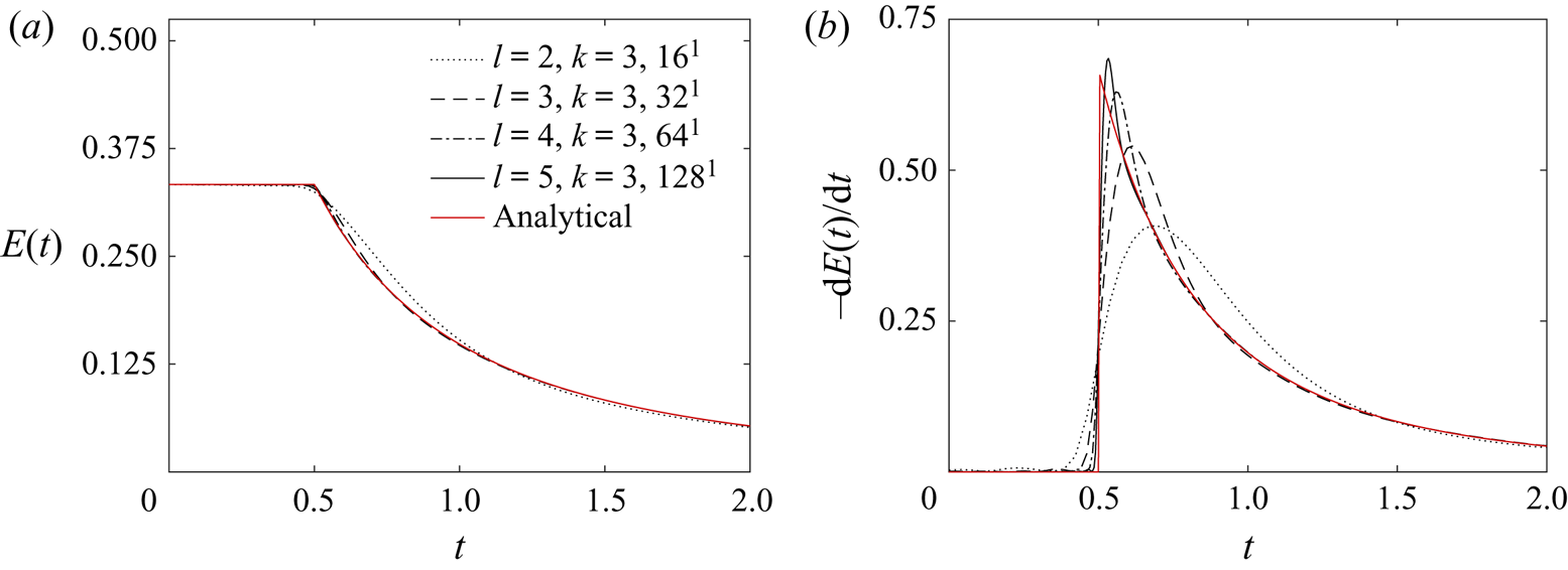
 $\nu \rightarrow 0$. In figure 3, we show results for both the kinetic energy and the dissipation rate for a sequence of mesh refinement levels of
 $l=2,\ldots, 5$ with degree
 $k=3$, resulting in effective resolutions of
 $16^1,\ldots,128^1$. For increasing spatial resolution, the numerical results converge to the analytical profiles. It can be seen that achieving grid-convergence for the dissipation rate requires higher spatial resolutions than for the temporal evolution of the kinetic energy itself. This is expected since the dissipation rate contains a temporal derivative that results in higher sensitivity to deviations (here numerical discretisation error) from the exact solution.
One-dimensional inviscid Burgers equations with hat function as initial condition: temporal evolution of kinetic energy (a) as well as dissipation rate (b) and convergence towards analytical profile for a mesh refinement study with refinement levels  $l=2,\ldots,5$ and polynomial degree
 $k=3$, resulting in effective resolutions of
 $16^1,\ldots,128^1$.

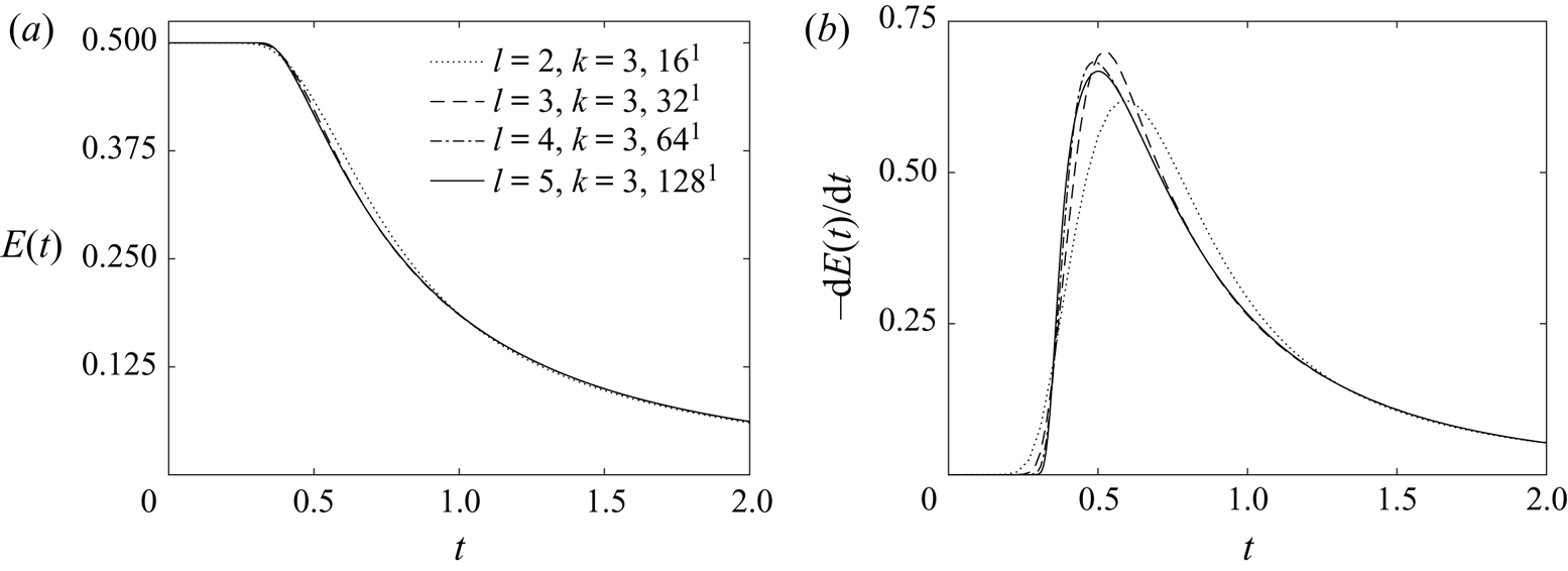
Figure 4 shows the same results for the problem with sine function as initial condition. We observe that the onset of energy dissipation is smooth, as opposed to the case of the hat function, where the kinetic energy exhibits a kink and the dissipation rate a jump at the time of the singularity. In other words, the occurrence of a finite-time singularity does not imply an instantaneous onset of dissipation. We keep this in mind when considering the three-dimensional inviscid Taylor–Green problem, which is a problem that also starts from sine-like initial data.
One-dimensional inviscid Burgers equations with sine function as initial condition: temporal evolution of kinetic energy (a) as well as dissipation rate (b) and mesh refinement study with refinement levels  $l=2,\ldots,5$ and polynomial degree
 $k=3$, resulting in effective resolutions of
 $16^1,\ldots,128^1$.

The point that we want to make with this example is that a discretisation scheme that involves purely numerical mechanisms of dissipation can provide the physically correct amount of dissipation for a sufficiently fine spatial resolution; see also the discussion in the introduction. Note that this is fundamentally different from viscosity solutions  $u^{\nu }$ for small
 $\nu > 0$, for which the required dissipation is realised by the additional viscous term in the equations and for which the dissipation stemming from the numerical discretisation scheme tends to zero if the mesh resolves the viscosity solution
 $u^{\nu }$ exhibiting steep but finite gradients. Although the one-dimensional Burgers equation cannot reflect the complexity of three-dimensional turbulent flows, these results provide confidence that numerical discretisation schemes can also predict the solution in a physically correct way for the higher-dimensional problems studied below.
3.3. Two-dimensional shear layer problem
We consider the two-dimensional shear layer roll-up problem (Brown Reference Brown1995) where the initial velocity is given as
 \begin{equation} \boldsymbol{u}(\boldsymbol{x},t=0) = \left( \tanh \left(\rho (0.25 - \vert x_2-0.5 \vert) \right), \delta \sin \left( 2{\rm \pi} x_1\right) \right)^{\mathsf{T}}. \end{equation}
Following Brown (Reference Brown1995), we set the two parameters  $\rho, \delta$ to
 $\rho = 30$ and
 $\delta = 0.05$. The problem is solved on the domain
 $\varOmega = [0,1]^2$ with periodic boundaries in both directions. In the following, different viscous simulations with viscosities
 $\nu = 2.5 \times 10^{-3}, 10^{-3}, 10^{-4}$ are considered, as well as the inviscid limit with
 $\nu =0$. The mesh is uniform Cartesian with
 $(2^l)^2$ elements for refinement level
 $l$, and the polynomial degree of the shape functions is
 $k=7$, resulting in the effective resolution of
 $( (k+1) 2^l )^2$. The simulations are run for the time interval
 $0 \leq t \leq 4$. The time step size is adapted dynamically with a Courant number of
 ${Cr}=0.25$.
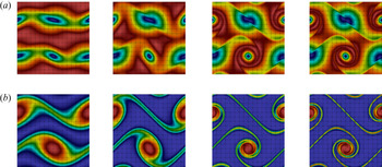
The aim of this example is to verify the robustness and accuracy of the present high-order DG discretisation for a simple two-dimensional example. As mentioned in the introduction, the energy is conserved for the two-dimensional incompressible Euler equations, and this property should be preserved by a consistent discretisation scheme for sufficiently fine spatial resolutions. Figure 5 shows contour plots of velocity magnitude and vorticity magnitude at time  $t=1.2$ for a mesh with
 $16^2$ elements (refinement level
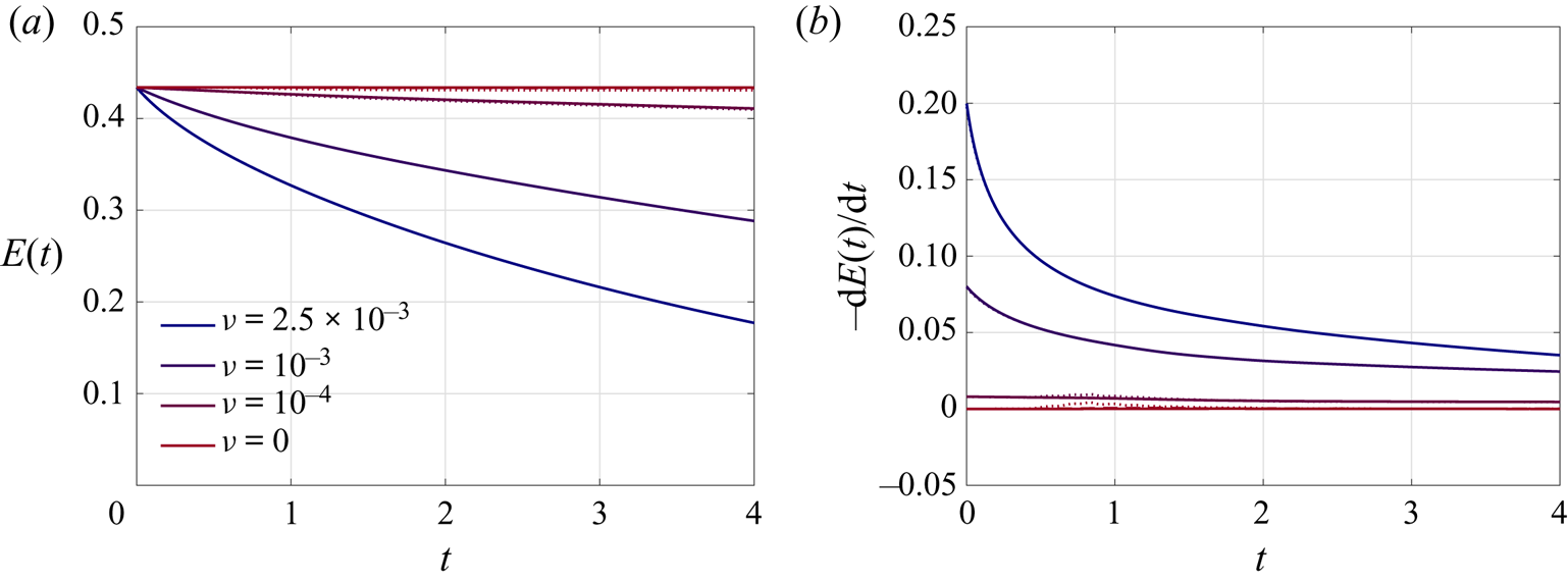
 $l=4$) for different values of the viscosity. In figure 6, we show the temporal evolution of the kinetic energy and the kinetic energy dissipation rate for the different viscosity values. For each viscosity, results obtained on three meshes of increasing resolution with
 $4^2$,
 $8^2$ and
 $16^2$ elements are shown. For large viscosities,
 $\nu = 2.5 \times 10^{-3}$ and
 $10^{-3}$, the results for the temporal evolution of the kinetic energy and dissipation rate coincide for all meshes. For the smallest viscosity of
 $\nu = 10^{-4}$ and the inviscid limit
 $\nu =0$, the results obtained on the two finest meshes coincide, and only minor deviations can be observed for the coarsest mesh. This is in qualitative agreement with the contour plots for the velocity magnitude in figure 5, which demonstrate that the velocity field is smooth and well resolved on the finest mesh for all viscosities. The resolution requirements are higher for the vorticity containing spatial derivatives of the velocity field. As already noted in Brown (Reference Brown1995), the vorticity field is still not well resolved even if convergence has already been achieved for the velocity or kinetic energy. It can be seen from figure 5 that the vorticity field is well resolved for the viscous cases
 $\nu = 2.5 \times 10^{-3}, 10^{-3}, 10^{-4}$, but shows grid-dependence with numerical artefacts in the form of elevations of the vorticity at the element corners, especially in the thin shear layer, which is most difficult to resolve. In agreement with what is expected physically, the kinetic energy dissipation rate tends to zero for
 $\nu \rightarrow 0$, and the kinetic energy is conserved in the inviscid limit
 $\nu =0$. Of particular importance with respect to the interpretation of results shown in § 3.4 for the three-dimensional Taylor–Green problem is the observation that the numerical dissipation occurring in the inviscid limit
 $\nu =0$ for coarse spatial resolutions decreases to zero under mesh refinement for this two-dimensional problem.
Two-dimensional shear layer roll-up problem: contour plots of velocity magnitude and vorticity magnitude at time  $t=1.2$ for four different values of the viscosity (blue indicates low value and red high value). The results shown correspond to a mesh with
 $16^2$ elements with a polynomial degree of
 $k=7$ (effective resolution
 $128^2$). (a) Velocity magnitude for
 $\nu =2.5 \times 10^{-3}, 10^{-3}, 10^{-4}, 0$ (from left to right). (b) Vorticity magnitude for
 $\nu =2.5 \times 10^{-3}, 10^{-3}, 10^{-4}, 0$ (from left to right).

Two-dimensional shear layer roll-up problem: temporal evolution of kinetic energy (a) and kinetic energy dissipation rate (b) for decreasing viscosity values of  $\nu = 2.5 \times 10^{-3}, 10^{-3}, 10^{-4}, 0$. For each viscosity, results are shown for effective resolutions of
 $32^2$ (dotted lines),
 $64^2$ (dashed lines) and
 $128^2$ (solid lines), corresponding to meshes with
 $4^2$,
 $8^2$ and
 $16^2$ elements with polynomial degree
 $k=7$.

An important aspect concerns the numerical robustness of the discretisation scheme. In Chalmers et al. (Reference Chalmers, Agbaglah, Chrust and Mavriplis2019), instabilities are reported for the same shear layer problem with viscosity  $\nu =0$ for a DG discretisation with polynomial degree
 $k=7$ and refinement level
 $l=4$. This originates from the fact that the stabilised discretisation techniques developed in Krank et al. (Reference Krank, Fehn, Wall and Kronbichler2017) and Fehn et al. (Reference Fehn, Wall and Kronbichler2018b) that render the discretisation robust in under-resolved scenarios and that are used in the present work are not applied in Chalmers et al. (Reference Chalmers, Agbaglah, Chrust and Mavriplis2019). No robustness problems have been observed for the present discretisation scheme, even for the coarsest resolutions, e.g. refinement levels of
 $l=0,1$ not shown explicitly here. This is a prerequisite for obtaining a feasible incompressible flow solver for three-dimensional turbulent flow problems that are even more challenging in terms of the stability of a numerical discretisation scheme. Instabilities have also been reported for continuous spectral element discretisations for this two-dimensional shear layer problem, where filtering techniques can be used to recover stability (Fischer & Mullen Reference Fischer and Mullen2001), at the cost of introducing new parameters into the discretisation scheme. A recent study by Thalabard, Bec & Mailybaev (Reference Thalabard, Bec and Mailybaev2020) uses a pseudo-spectral scheme with hyperviscous linear dissipation to investigate a two-dimensional Kelvin–Helmholtz problem. A discretisation technique with properties similar to the present stabilised DG discretisation in terms of robustness and accuracy are exactly divergence-free
 $H$(div)-conforming discretisations; see for example the studies by Guzmán, Shu & Sequeira (Reference Guzmán, Shu and Sequeira2016) and Fu (Reference Fu2019) analysing this shear-layer problem, the study by Schroeder & Lube (Reference Schroeder and Lube2018) discussing other two-dimensional examples, such as the Kelvin–Helmholtz instability problem, and the study by Fehn et al. (Reference Fehn, Kronbichler, Lehrenfeld, Lube and Schroeder2019) comparing
 $H$(div)- and stabilised
 $L^2$-conforming discretisations for three-dimensional turbulent flow problems in under-resolved scenarios.
3.4. Three-dimensional Taylor–Green vortex problem
We consider the three-dimensional Taylor–Green vortex problem (Taylor & Green Reference Taylor and Green1937) defined by the following initial velocity field:
 \begin{equation} \boldsymbol{u}(\boldsymbol{x},t=0) = \left( \sin x_1 \cos x_2 \cos x_3, - \cos x_1 \sin x_2 \cos x_3, 0 \right)^{\mathsf{T}}. \end{equation}
Results of viscous simulations for increasing Reynolds number  $Re={1}/{\nu }$ are given in figure 1. In the following, the focus is entirely on the inviscid limit
 $\nu =0$. The simulations are run over the time interval
 $0\leq t \leq T = 20$ to cover the different flow regimes of laminar flow, transition to turbulence and decaying turbulence. To reduce computational costs for fixed resolution of the flow (or to increase the effective resolution for a given computational cost), it is common practise to exploit the symmetry of the Taylor–Green problem and simulate the flow on the impermeable box
 $\varOmega = [0, {\rm \pi}]^3$ with symmetry boundary conditions on all boundaries (Brachet et al. Reference Brachet, Meiron, Orszag, Nickel, Morf and Frisch1983), i.e.
 \begin{equation} \boldsymbol{u}\boldsymbol{\cdot} \boldsymbol{n} = 0,\quad \frac{\partial \boldsymbol{u}}{\partial n} = 0, \end{equation}
as opposed to the periodic box  $\varOmega = [-{\rm \pi}, {\rm \pi}]^3$ that is also used in computational studies. This optimisation allows us to reduce computational costs by a factor of
 $8$ for the present DG discretisation. Further symmetries can be exploited by spectral methods leading to the so-called fundamental box (Brachet et al. Reference Brachet, Meiron, Orszag, Nickel, Morf and Frisch1983; Kida Reference Kida1985).
The computational domain  $\varOmega = [0 , {\rm \pi}]^3$ is discretised using a uniform Cartesian grid consisting of
 $(2^l)^d$ elements, where
 $l$ denotes the level of refinement. The number of unknowns is given as
 $N_{{DoFs}}=(2^l)^d(d(k_u+1)^d+(k_p+1)^d)=(2^l)^d(d(k+1)^d+k^d)$. It is common practise in the literature to express the effective mesh resolution in terms of the periodic box to obtain comparability between different discretisation techniques that exploit different levels of symmetry. Hence, we define the effective spatial resolution as
 $(2^{l+1}(k+1))^d$; e.g. the effective resolution is
 $64^3$ for refinement level
 $l=3$ and polynomial degree
 $k=3$. Absolute tolerances of
 $10^{-12}$ and relative tolerances of
 $10^{-6}$ are used for the iterative linear solvers, where relative tolerance means that the residual is reduced by a factor of
 $10^{-6}$ compared to the initial residual that uses as initial guess a high-order extrapolation of the solution from previous time steps. The polynomial degree used for the Taylor–Green vortex simulations is
 $k=3$, and adaptive time stepping with
 ${Cr}=0.25$ is used for all simulations. The penalty factors of the divergence and continuity penalty terms are chosen as defined in Fehn et al. (Reference Fehn, Wall and Kronbichler2018b), except for the finest resolution of
 $8192^3$, where the penalty factors have been increased by a factor of
 $\zeta =2$ compared to the standard definition. For this fine resolution, the simulation also remained stable for the default value of
 $\zeta = 1$, but we observed oscillations in the maximum vorticity at early times, giving an indication of the need for a slightly larger penalisation of the divergence-free constraint and normal continuity of the velocity field. Since these oscillations disappeared when increasing the penalty factors by a factor of
 $2$, this value was ultimately used for this highest-resolution simulation. The highest resolution of
 $8192^3$ has
 $N_{{DoFs}}=2.35 \times 10^{11}$ unknown degrees of freedom, and
 $2.27 \times 10^{5}$ time steps were solved during this simulation. The computations were performed on a large supercomputer using almost
 $100\,\mathrm {k}$ cores for the highest resolution, requiring a run time of approximately
 $8.4$ days.
3.4.1. Recapitulating the state of the art
This section briefly summarises the type of discretisation, the maximal effective resolutions and the final time  $T$ of the simulations considered in previous numerical studies for the three-dimensional inviscid Taylor–Green vortex problem. In Brachet et al. (Reference Brachet, Meiron, Orszag, Nickel, Morf and Frisch1983), a spectral method with maximum resolution of
 $256^3$ (exploiting symmetry) was used, and direct simulation was performed up to times
 $t \leq 4$. In a subsequent work by Brachet et al. (Reference Brachet, Meneguzzi, Vincent, Politano and Sulem1992), a maximum resolution of
 $864^3$ (exploiting symmetry) was reached, and again direct simulation was performed up to times
 $t \leq 4$. A comparison of a spectral method and a weighted essentially non-oscillatory (WENO) finite difference method can be found in Shu et al. (Reference Shu, Don, Gottlieb, Schilling and Jameson2005), where a maximum resolution of
 $368^3$ (exploiting symmetry) and simulation up to times
 $t \leq 6$ is considered. A modal DG method was studied in Chapelier et al. (Reference Chapelier, De La Llave Plata and Renac2012), with the simulations performed up to times
 $t\approx 5 - 7$, until they became unstable, with the maximum resolution of around
 $96^3$ for polynomial degrees from
 $k=1$ to
 $k=5$. DG discretisations used to study the inviscid Taylor–Green vortex problem have also been analysed in Moura et al. (Reference Moura, Mengaldo, Peiró and Sherwin2017a,Reference Moura, Mengaldo, Peiró and Sherwinb), Fernandez, Nguyen & Peraire (Reference Fernandez, Nguyen and Peraire2018), Manzanero et al. (Reference Manzanero, Ferrer, Rubio and Valero2020) and Schroeder (Reference Schroeder2019), but with a focus on large eddy simulation (LES) modelling. The study by Cichowlas & Brachet (Reference Cichowlas and Brachet2005) used a spectral method with maximum resolution of
 $2048^3$, with simulations performed up to times
 $t \leq 4$. The highest resolution of
 $4096^3$ was achieved by Bustamante & Brachet (Reference Bustamante and Brachet2012) using a spectral method, and the simulations were performed up to times
 $t \leq 4$.
In these works, indications of finite-time singularities are mentioned. In Morf et al. (Reference Morf, Orszag and Frisch1980),  $t_* = 5.2$ is obtained from power series expansions. A more accurate variant using power series expansions presented in Brachet et al. (Reference Brachet, Meiron, Orszag, Nickel, Morf and Frisch1983) leads to
 $t_* = 4.4 \pm 0.2$. Furthermore, the study by Brachet et al. (Reference Brachet, Meiron, Orszag, Nickel, Morf and Frisch1983) reports indirect evidence for a finite-time singularity according to the direct numerical simulation results, but the authors conclude that the resolution of
 $256^3$ is not sufficient to investigate the occurrence of finite-time singularities for times
 $t \geq 4$. The more recent study by Bustamante & Brachet (Reference Bustamante and Brachet2012) estimates a blowup time of
 $t_* \approx 4$ and concludes that the results are not inconsistent with the occurrence of a singularity. The work of Larios et al. (Reference Larios, Petersen, Titi and Wingate2018) obtains a blowup time of
 $t_* \approx 4.2$, similar to the blowup time in Brachet et al. (Reference Brachet, Meiron, Orszag, Nickel, Morf and Frisch1983).
3.4.2. Results in physical space
The early stage of the Taylor–Green vortex evolution with the formation of thin flow structures is visualised in figure 7. Similar results are shown and discussed in detail in Brachet et al. (Reference Brachet, Meiron, Orszag, Nickel, Morf and Frisch1983), for the same effective resolution of  $256^3$, using a spectral method. In agreement with the above results for the two-dimensional shear layer problem, we observe that the velocity field is resolved at all times, while under-resolution effects are clearly visible in the contour plots of the vorticity magnitude at later times
 $t=3$ and
 $t=4$ for the chosen resolution. A high-resolution visualisation of the thin vortex sheet shown in figure 7 with a volume rendering of the vorticity magnitude is shown in Bustamante & Brachet (Reference Bustamante and Brachet2012) for an effective resolution of
 $4096^3$. Figure 8 shows visualisation results for a high-resolution simulation (effective resolution
 $2048^3$) at later times
 $t=4,5,6,7,8,9$, around which small-scale features occur and transition to turbulence takes place. These results illustrate that the present discretisation scheme does not lead to thermalisation, which appears to be a prerequisite for obtaining physically meaningful results; compare for example the present results to the thermalised results shown in Schroeder (Reference Schroeder2019, figure 9.14). Flow visualisation is discussed in the literature as one possibility for tracing finite-time singularities, but appears to be impractical due to the difficulties in handling large data sets for high-resolution simulations necessary for such investigations, as well as the difficulties in visualising singularities (which do not show up as singularities for a finite-resolution numerical simulation). Hence, our attention is turned to other techniques in the following.
Three-dimensional inviscid Taylor–Green problem: contour plots of velocity magnitude and vorticity magnitude (blue indicates low value and red high value) on plane  $x={\rm \pi}$ of impermeable box. The results shown correspond to a mesh with
 $32^3$ elements with a polynomial degree of
 $k=3$ for the shape functions (effective resolution
 $256^3$). (a) Velocity magnitude on plane
 $x={\rm \pi}$ at times
 $t=0,1,2,3,4$ (from left to right). (b) Vorticity magnitude on plane
 $x={\rm \pi}$ at times
 $t=0,1,2,3,4$ (from left to right).

Three-dimensional inviscid Taylor–Green problem: isosurfaces of Q-criterion at times  $t=4,5,6,7,8,9$, where the blue surface corresponds to a value of
 $-0.5$ and the orange surface to a value of
 $0.5$. The results correspond to a mesh with
 $256^3$ elements with a polynomial degree of
 $k=3$ for the shape functions (effective resolution
 $2048^3$). Results are shown for (a)
 $t=4$; (b)
 $t=5$; (c)
 $t=6$; (d)
 $t=7$; (e)
 $t=8$; (f)
 $t=9$.

We present numerical results of a mesh convergence study for refinement levels  $l=3,\ldots,10$ and polynomial degree
 $k=3$. Figure 9 shows the temporal evolution of the kinetic energy and the kinetic energy dissipation rate. At small times
 $t$, the energy is constant and the energy dissipation rate is zero. This agrees with the expected theoretical behaviour stating energy conservation as long as the solution remains smooth and has also been shown in previous works in a similar way. In this work, we do not want to terminate the simulations once we expect them to become under-resolved, but instead continue the simulations until
 $t=20$. Depending on the effective mesh resolution, an onset of energy dissipation can be observed that shifts towards later times for increasing spatial resolution. However, this time of onset of dissipation does not seem to be pushed beyond
 $t\approx 5$ even for the finest spatial resolutions. This is illustrated more clearly in figure 10, which plots the kinetic energy dissipation rate in logarithmic scaling as well as the error against the fine-resolution simulation (ref). The fact that the dissipation rate of the simulations with resolutions of
 $2048^3$ and
 $4096^3$ ‘converges’ to that of the finest resolution at a time
 $t \approx 5$ for
 $2048^3$ and
 $t < 5$ for
 $4096^3$ is consistent with a potential blowup time
 $t_* < 5$, in our opinion. Overall, we make the interesting phenomenological observation that the kinetic energy evolution and its dissipation rate tend to converge to a dissipative solution rather than an energy-conserving solution with vanishing dissipation rate. As in high-Reynolds-number viscous simulations of this problem, the kinetic energy dissipation rate reaches a maximum at
 $t =8 - 9$ and decreases afterwards. In § 3.4.5, grid-convergence of the sequence of discrete solutions to a dissipative reference solution is investigated in more detail. Note that the present results for the dissipation rate agree well with those of Cichowlas et al. (Reference Cichowlas, Bonaïti, Debbasch and Brachet2005) for an energy-conserving scheme, where an effective dissipation rate is deduced from the thermalised energy
 $E_{{th}}(t)$, the energy associated with the small scales with wavenumber
 $k > k_{{th}}$, where
 $k_{{th}}$ is the wavenumber at which the energy spectrum exhibits a local minimum.
Three-dimensional inviscid Taylor–Green problem: temporal evolution of kinetic energy (a) and kinetic energy dissipation rate (b) for increasing effective spatial resolution.

Three-dimensional inviscid Taylor–Green problem: temporal evolution of kinetic energy dissipation rate in logarithmic scaling (a) and error against fine-resolution simulation (b).

It is now examined whether this behaviour is consistent with the temporal evolution of the maximum vorticity and the enstrophy shown in figure 11. For both quantities, one can immediately identify three phases: (i) a first phase up to approximately  $t \approx 3$ in which the flow is well resolved for all spatial resolutions, so that the results essentially overlap for all simulations, (ii) an intermediate phase
 $3 < t < 5$ in which the different simulations start to deviate from each other, due to under-resolution effects depending on the spatial resolution of each simulation, and (iii) a final phase
 $t > 5$ in which the results of all simulations deviate substantially, due to the different resolution capabilities of the simulations. In the first phase, the vorticity first decreases, reaches a minimum and then begins to grow exponentially, in agreement with the results in Bustamante & Brachet (Reference Bustamante and Brachet2012, figure 1(b)). In figure 11, we have added a reference curve with
 $\exp (\frac {2}{3} t)$ growth which describes the growth of the maximum vorticity very well in this regime. In the second phase, at around
 $t \approx 3.5$, the maximum vorticity begins to grow substantially faster, and the growth of vorticity essentially depends on the spatial resolution, which is directly linked to the maximum velocity gradient that can be represented on a given mesh. As already mentioned in the introduction, for every simulation that does not blow up due to numerical instabilities of a discretisation scheme, the maximum vorticity will remain finite no matter how fine the spatial resolution is. Therefore, the occurrence of a finite-time singularity with
 $\lim _{t\rightarrow t_*} \Vert \boldsymbol {\omega } \Vert _{\infty } = \infty$ remains speculative. While our results might be considered consistent with such a vorticity blowup scenario, we are not able to identify a concrete blowup time
 $t = t_*$ from the present results. We instead observe that the time of maximum vorticity observed in this second phase is shifted to later times for the finest spatial resolutions as well. At the same time, one might argue that a finite-time blowup at a time
 $t = t_*$ with
 $t_* \approx 4 - 5$ would produce results similar to those shown here, with the maximum vorticity following the exact profile until the curve of a specific spatial resolution branches off due to under-resolution of the simulation. In such a scenario, one would expect the maximum vorticity to grow by a factor of
 $2$ for refinement level
 $l \rightarrow l+1$ due to the mesh size being reduced by a factor of
 $2$, allowing numerical gradients to become twice as large. While we observe such an increase in maximum vorticity from one refinement level to the next, it is not clear whether this suspected blowup would happen in finite time. In the third phase, the maximum vorticity reaches a global maximum between
 $t=6$ and
 $t=7$ for each resolution before it starts to decrease slowly. In this phase, the maximum vorticity is offset by a factor of approximately
 $2$ from one refinement level to the next. This is a clear indication that none of the simulations is able to resolve the finest structures, and it is plausible that a factor of
 $2$ in mesh size also gives a factor of
 $2$ in maximum vorticity. Finally, the maximum vorticity shows strongly fluctuating behaviour in the third phase. Note that the maximum vorticity is determined numerically by taking the maximum over all quadrature points, i.e. the vorticity field is sampled in discrete points. This effect is negligible for well-resolved scenarios but might explain oscillatory behaviour in case a local maximum travels through the domain.
Three-dimensional inviscid Taylor–Green problem: temporal evolution of maximum vorticity (a) and enstrophy (b) for increasing effective spatial resolution.

The temporal evolution of the enstrophy is overall similar to that of the maximum vorticity. An important difference is that the enstrophy does not reach a local minimum at early times as observed for the maximum vorticity. In the second phase, the growth of the enstrophy is more moderate than that of the maximum vorticity. In the third phase, the enstrophy curves can be described essentially as smoothed variants of the maximum vorticity from which the high-frequency content has been removed. A possible explanation for the enstrophy behaviour in the second and third phases is that the enstrophy is not a local quantity, but an average in space over the computational domain. Again, a growth in enstrophy by a factor of two from one mesh level to the next is observed at later times, which is consistent with an enstrophy evolution theoretically taking infinite values, or taking values that are finite but much larger than those obtained numerically in figure 11. Considering Onsager's conjecture as valid, it is clear that one cannot expect convergence for the temporal evolution of maximum vorticity and enstrophy. Theoretically, convergence can then only be expected for the kinetic energy evolution and to some extent for kinetic energy spectra up to the resolution limits of the discretisation scheme, as discussed in the following.
3.4.3. Results in spectral space
Figure 12 shows kinetic energy spectra for increasing spatial resolution at various instants of time, namely at  $t=1,\ldots,9$ in steps of width
 $1$. Results are shown for resolutions of
 $128^3$ to
 $2048^3$. The high computational costs and memory requirements of the fast Fourier transformation part of our simulations prevented the spectral analysis for the highest resolutions of
 $4096^3$ and
 $8192^3$. For a discussion of the general behaviour of energy spectra as a function of time at early times
 $t\leq 4$, we refer to Brachet et al. (Reference Brachet, Meiron, Orszag, Nickel, Morf and Frisch1983), Cichowlas & Brachet (Reference Cichowlas and Brachet2005) and Bustamante & Brachet (Reference Bustamante and Brachet2012), where it is shown how the energy spectra can be fitted to functions of the form
 $E(k,t) = C(t) k^{-n(t)}\exp ( - 2k \delta (t))$, and where values obtained for
 $n(t)$ and
 $\delta (t)$ are discussed in detail. To verify the present results, we include reference curves of slope
 $n = 3$ (blowup of enstrophy) and
 $n = 5/3$ (Kolmogorov's inertial scaling law) or
 $n = 7/3$ (motivated by results obtained in Piatkowski (Reference Piatkowski2019) for viscous Taylor–Green simulations). The energy spectra are compared against the slope
 $n = 3$ as a means of investigating the plausibility of potentially singular behaviour and to identify a time
 $t = t_*$ at which such a blowup could occur, as motivated in § 3.1. Once the flow has transitioned to a fully turbulent state, the energy spectrum can be expected to exhibit some form of Kolmogorov scaling. For this purpose, we consider the energy spectra at times
 $t=8$ and
 $t=9$, where the maximum dissipation rate occurs, even though the flow might not be fully homogeneous isotropic at those times, and the results might deviate from Kolmogorov's
 $k^{-5/3}$ scaling. To quantify the resolution capabilities of the present discretisation, we also plot the Nyquist wavenumber
 $k_{{Nyquist}}$, as well as the wavenumber
 $k_{1\,\%}$ according to the
 $1\,\%$ rule of Moura et al. (Reference Moura, Mengaldo, Peiró and Sherwin2017b), which aims to obtain an accurate resolution limit for upwind-like DG discretisations for a specific polynomial degree of the function space.
Three-dimensional inviscid Taylor–Green problem: kinetic energy spectra for effective resolutions of  $128^3, 256^3, 512^3$ at times
 $t=1,2,\ldots,9$. (a) Effective resolution of
 $128^3$. (b) Effective resolution of
 $256^3$. (c) Effective resolution of
 $512^3$.

Three-dimensional inviscid Taylor–Green problem: kinetic energy spectra for effective resolutions of  $1024^3, 2048^3$ at times
 $t=1,2,\ldots,9$. (d) Effective resolution of
 $1024^3$. (e) Effective resolution of
 $2048^3$.

Figure 12 shows that the range of scales resolved by the numerical method increases with increasing spatial resolution as expected theoretically, and that the resolution limit for polynomial degree  $3$ is described very well by the
 $1\,\%$ rule corresponding to this degree. The energy spectra reach a slope of
 $-3$ between
 $t=4$ and
 $t=5$, making our results consistent with the occurrence of singular behaviour around that time (
 $4 < t_* < 5$), in agreement with the rapid growth of the maximum vorticity observed in the same time interval; see figure 11. The spectra in the inertial range show a decay slightly stronger than
 $k^{-5/3}$, and better agreement is achieved when they are compared to the
 $k^{-7/3}$ scaling that is also shown in figure 12. This behaviour has already been observed in Piatkowski (Reference Piatkowski2019) for viscous Taylor–Green vortex simulations, where it was found that Kolmogorov's
 $k^{-5/3}$ scaling can only be observed at later times, e.g.
 $t \approx 20$. Regarding the inertial scaling, the present results are therefore in agreement with results in the literature. Towards the Nyquist wavenumber, a moderate pile-up of energy can be observed by comparison against the
 $-5/3$ and
 $-7/3$ references slopes before the energy falls off very rapidly. The energy pile-up is characteristic of this type of high-order DG approach and becomes stronger for higher polynomial degrees; see Moura et al. (Reference Moura, Mengaldo, Peiró and Sherwin2017a,Reference Moura, Mengaldo, Peiró and Sherwinb) and references therein. This particular behaviour is often the primary target when optimising discretisation schemes; see for example the recent studies by Flad & Gassner (Reference Flad and Gassner2017), Winters et al. (Reference Winters, Moura, Mengaldo, Gassner, Walch, Peiro and Sherwin2018) and Manzanero et al. (Reference Manzanero, Ferrer, Rubio and Valero2020) and references therein, which suggest counteracting this energy bump behaviour with explicit subgrid scale modelling. However, the recent study by Fernandez et al. (Reference Fernandez, Nguyen and Peraire2018) shows that this topic is delicate, and improvements in some quantities through the use of explicit subgrid models cause deviations in other quantities, such as the temporal evolution of the kinetic energy dissipation rate. In our opinion, the challenge lies in improving the spectral behaviour and at the same time not giving up the improved resolution capabilities (per degrees of freedom) of high-order discretisations. The overall goal can be formulated as the achievement of a discretisation method that is accurate with respect to both the spectral behaviour and the behaviour in physical space, e.g. the temporal evolution of the kinetic energy and its dissipation rate. We want to note that from such a holistic viewpoint it is not clear a priori whether an explicit subgrid scale model optimising the energy spectrum according to the inertial
 $k^{-5/3}$ law is advantageous overall. We take up this point again in § 4, where we discuss possible directions of future research. The energy spectra shown in Schroeder (Reference Schroeder2019, figure 9.15) for an exactly energy-conserving discretisation scheme illustrate that such a scheme leads to physical inconsistencies for the
 $E(k)$ curves in the inertial range.
3.4.4. Does the numerical dissipation have artificial or predictive character?
The dissipation of kinetic energy observed for the inviscid Taylor–Green simulations originates from the numerical method. At first sight, one might argue that changing the discretisation scheme by choosing another numerical flux or varying certain parameters would lead to more or less dissipative results, i.e. that the amount of dissipation is artificial and is determined by the discretisation parameters. The results of the mesh convergence study shown above do not support this point of view, and we want to provide further results that might allow insight into the predictive character of these dissipative numerical solutions. In this context, it is illustrative to study the temporal evolution of the kinetic energy and its dissipation rate under a variation of parameters of the discretisation scheme. Figure 13 shows a parameter study of the penalty factor  $\zeta$ of the divergence and continuity penalty terms of the present discretisation, considering values of
 $\zeta = 1,2,4,8$ for the example of the
 $1024^3$ spatial resolution. Note that this parameter is the crucial one in stabilising the method in the under-resolved and high-Reynolds regime (Fehn et al. Reference Fehn, Wall and Kronbichler2018b, Reference Fehn, Kronbichler, Lehrenfeld, Lube and Schroeder2019). We observe that both the overall amount of dissipation and the dissipation maximum are essentially unaltered by variation of this parameter. It is worth noting that the time of onset of dissipation is also not affected by the value of
 $\zeta$. This might have important implications. Assuming that a non-dissipative (energy-conserving) solution is the correct physical behaviour and that the numerical dissipation is artificial, one might expect an increase of the penalty parameter to affect the numerical solution more strongly, e.g. to change the amount of overall dissipation, or to lead to a delayed onset of dissipation due to better fulfilment of the divergence-free constraint. As we do not observe such behaviour, in our opinion these results are an indication that the obtained dissipative solutions have a predictive character. It is clear that we cannot expect the results to be identical for different penalty factors, since the results are not grid-converged for the chosen resolution of
 $1024^3$, meaning that the discretisation scheme and its parameters affect the numerical solution.
Three-dimensional inviscid Taylor–Green problem: variation of penalty factor  $\zeta$ and its influence on the temporal evolution of the kinetic energy (a) and the kinetic energy dissipation rate (b) for an effective resolution of
 $1024^3$.

3.4.5. Are the results grid-converged?
We finally address the question of whether and to what extent the results presented for inviscid Taylor–Green simulations can be considered grid-converged. For this purpose, we compute relative  $L^2$-errors for the kinetic energy evolution and the kinetic energy dissipation rate,
 \begin{equation} e_{E}^2 = \frac{\displaystyle\int_{t=0}^{\textrm{T}} \left(E(t) - E_{{ref}}(t) \right)^{2}\mathrm{d}t}{\displaystyle\int_{t=0}^{\textrm{T}} \left( E_{{ref}}(t) \right)^{2} \mathrm{d}t},\quad e_{\mathrm{d}E/\mathrm{d}t}^2 = \frac{\displaystyle\int_{t=0}^{\textrm{T}} \left( \frac{\mathrm{d}E(t)}{\mathrm{d}t} - \frac{\mathrm{d}E_{{ref}}(t)}{\mathrm{d}t} \right)^{2} \mathrm{d}t}{\displaystyle\int_{t=0}^{\textrm{T}} \left( \frac{\mathrm{d}E_{{ref}}(t)}{\mathrm{d}t} \right)^{2} \mathrm{d}t}. \end{equation}
Since no analytical solution is available, the errors are measured using the finest resolution of  $8192^3$ as a reference (ref). This implies that we cannot compute the error for the
 $8192^3$ resolution. The error of this simulation can only be roughly estimated by extrapolating the convergence trend observed for the coarser resolutions and assuming that this convergence behaviour continues for the finest resolution. Defining a simulation with a relative error of
 $1\,\%$ or less as grid-converged, we see from the results in figure 14 that we achieve grid-convergence in the kinetic energy evolution, with errors below
 $1\,\%$. For the second finest resolution (the last data point in figure 14), the measured error is
 $0.27\,\%$. For the kinetic energy dissipation rate, the error is significantly larger, demonstrating that this quantity is more sensitive, in agreement with what has been observed in figure 1. For the second finest resolution, the measured error is
 $3.52\,\%$. While the errors can be expected to be smaller for the finest resolution of
 $8192^3$ that is used as a reference solution here, we conclude that even finer resolutions would be required to achieve grid-convergence (in terms of the
 $1\,\%$ error level) for the kinetic energy dissipation rate. Figure 14 also shows linear least-squares fits (e.g.
 $\log (E) \approx a \log (N_{{DoFs}}) + b$ for the kinetic energy) to the data obtained from the numerical experiments, where a mean convergence rate of approximately
 $h^{3/4}$ is obtained for the kinetic energy and
 $h^{1/2}$ for the dissipation rate. This result – seemingly providing numerical evidence of grid-convergence to a dissipative solution of the three-dimensional incompressible Euler equations under Taylor–Green initial conditions – is the main result of the present study. While one might conjecture that this solution could be a weak Euler solution, there is currently no rigorous mathematical theory guaranteeing convergence to a weak solution. Moreover, even if we in fact obtained convergence to a weak Euler solution, it might not be the viscosity solution for
 $\nu \to 0$. Finally, the results in figure 14 cannot exclude the possibility that the dissipation rate would (slowly) tend to zero in the limit
 $h \to 0$ if finer spatial resolutions were realised. Let us explain this decisive aspect in more detail. For a solution that is non-dissipative (i.e. energy-conserving) from a physical perspective, one might argue that dissipation in the numerical simulation can originate only from under-resolution and can be expected to tend to zero when the resolution is increased. However, a dissipation rate decreasing extremely slowly under mesh refinement, e.g. as
 $1/\log \log (1/h)$, might then (erroneously) indicate grid-convergence to a dissipative solution, but the true solution is energy-conserving. Against this background, our numerical investigations according to the indirect approach are consistent with or suggestive of finite-time singularities, but do not conclusively provide evidence of finite-time singularities.
Three-dimensional inviscid Taylor–Green problem: relative  $L^2$-errors of the temporal evolution of the kinetic energy (a) and the kinetic energy dissipation rate (b) for effective resolutions ranging from
 $8^3$ to
 $4096^3$.

4. Conclusion and outlook
Hunting for finite-time singularities in incompressible Euler flows is a challenging discipline. Searching for singular behaviour in visualisations of three-dimensional simulation results evokes the picture of finding a needle in a haystack, as it can be expected that singularities are very localised and will never be resolved by a numerical scheme, and the amount of data for large-scale three-dimensional simulations soon becomes cumbersome. For this reason, most previous studies have focused on quantities such as the maximum vorticity, the analyticity strip width, fitting energy spectra to power law behaviour and related blowup criteria. The present work focuses on global quantities such as the temporal evolution of the kinetic energy, avoiding geometrical complexities in visualisation and striving for a clearer indication of singular behaviour, given that it might be computationally less demanding to resolve the kinetic energy than the vorticity in numerical simulations. We call this an indirect approach, since it exploits the connection between singular behaviour and anomalous energy dissipation according to Onsager's conjecture. A decisive point is that this technique requires suitable discretisation schemes that remain robust in the presence of singularities and provide mechanisms of dissipation in case no viscous dissipation is present, which is a challenge in itself. Then, the idea is that observing energy-dissipating behaviour for a sequence of mesh refinement levels provides insight into the physical dissipation behaviour of the problem under investigation.
We apply this technique to one-, two- and three-dimensional problems, obtaining results consistent with theory in one and two space dimensions. Subsequently, we use the technique to study the complex three-dimensional inviscid Taylor–Green problem, for which we observe energy-dissipating behaviour that is consistent with the high-Reynolds-number limit of viscous simulations available in the literature. The present study measures grid-convergence to a dissipative, fine-resolution numerical solution for the three-dimensional inviscid Taylor–Green problem with a measured relative  $L^2$-error of
 $0.27\,\%$ for the kinetic energy and
 $3.52\,\%$ for the kinetic energy dissipation rate. The results for the temporal evolution of the kinetic energy may therefore be considered to be grid-converged, and might serve as a reference solution for future studies. Regarding the temporal evolution of the maximum vorticity and the enstrophy, we are able to resolve an increase of almost four orders of magnitude for both quantities. To the best of our knowledge, these are the highest-resolution results published to date for the three-dimensional inviscid Taylor–Green vortex problem. Confidence in the reliability of the numerical results for this challenging three-dimensional problem is increased by the circumstance that the numerical method applied here is a robust discretisation scheme that remains numerically stable in the inviscid limit for all spatial resolutions that have been investigated. This is an important prerequisite for drawing conclusions about a potential physical blowup. In contrast, no conclusions can be drawn from a numerical simulation that blows up in finite time, since the observed blowup is due to numerical instabilities. In other words, a physical blowup does not imply a numerical blowup for a finite-resolution numerical simulation.
In summary, this work wants to raise the questions of (i) to what extent these results are related to weak dissipative solutions of the incompressible Euler equations, (ii) to what extent these results can then be interpreted as a numerical confirmation of the energy dissipation anomaly, and (iii) whether these results would imply finite-time singularities according to Onsager's conjecture. Let us emphasise that the present results do not formally prove convergence of the discrete velocity fields  $\boldsymbol {u}_h$ to a weak Euler solution
 $\boldsymbol {u}$. Even if convergence to a weak Euler solution had been obtained for a subsequence
 $h_j$, another subsequence
 $h_k$ might converge to a different weak Euler solution. Moreover, we cannot exclude the possibility that the observed ‘dissipation anomaly’ is of numerical origin, in the sense that the spatial resolutions considered here might be too coarse to adequately resolve an energy-conserving Euler solution. Nevertheless, the present study might complement theoretical and experimental works on anomalous energy dissipation and the related implications for finite-time singularities of three-dimensional incompressible Euler flows according to Onsager's conjecture. As part of future work, the so-called
 $4/5$th-law (Duchon & Robert Reference Duchon and Robert2000) should be investigated numerically in order to substantiate the hypothesis of having found a dissipative anomaly. Finally, the present work would gain further theoretical support from a proof of convergence to generalised weak Euler solutions for DG discretisation schemes of the Euler equations in the limit
 $h \to 0$ (along subsequences).
Given the challenges of the proposed indirect approach, it appears to be natural to raise the question of whether this technique has advantages over well-known direct techniques. Let us share some ideas about why the indirect approach might be an attractive technique for the exploration of finite-time singularities. A key motivation for the indirect approach is that it might not be necessary to resolve the smallest scales of the flow in order to resolve the temporal evolution of the kinetic energy. This is based on the observation that resolving the vorticity field (direct approach) typically requires significantly finer resolutions than resolving the kinetic energy (indirect approach). When studying singularities by the direct approach, one needs to realise that it is impossible to resolve the smallest scales through finite spatial resolutions. The vorticity will take finite values at all times for a stable discretisation scheme, so that results of a single simulation do not serve as numerical evidence of a finite-time singularity. (In this context, the term finite means that the quantity of interest takes values much smaller than the ‘infinite’ value defined by the maximum floating point number that can be represented on a computer.) A key element of the indirect approach is a mesh refinement study where the quantities of interest (kinetic energy and its dissipation rate) do not blow up. In our opinion, this circumstance supports cross-solver validation very naturally. Assume for example that different spatial discretisation schemes would converge to the same dissipative numerical solution (measured by some error norms as done in the present work). A cross-solver validation of the kinetic energy evolution or dissipation rate (indirect approach) might provide confidence that the obtained dissipative behaviour is not artificial (why should entirely different PDE solvers produce the ‘same’ artificial result with artificial dissipation?). In contrast, it would be difficult for each of these simulations to demonstrate a blowup of vorticity in order to provide evidence of finite-time singularities by direct techniques. All these solvers might show an increase in vorticity by a large factor, but it would still not be clear whether a finite-time singularity  $\Vert \boldsymbol {\omega } \Vert _{\infty } \to \infty$ occurs. Of course, sufficient data are not available currently in the literature to substantiate this assumption regarding a cross-solver validation of our results. One line of study that we want to initiate with the present contribution is exactly such a cross-solver validation, based on space-averaged results or other suitable statistical results. In summary, the argument in favour of the indirect approach would then be a clearer indication of finite-time singularities due to relaxed resolution requirements as compared to the direct approach.
The applicability of high-order DG discretisations to large-scale problems in turbulence research, for which spectral methods are currently the state of the art due to their accuracy and computational efficiency, has been demonstrated. Finally, the present study gives indications of what a promising large-eddy simulation strategy might be, and contributes to the long-lasting and difficult discussion on explicit versus implicit subgrid scale models. High-order discretisations that can be described as implicit LES have shown very promising results for moderate-Reynolds-number flows, but it is often argued that such techniques can ultimately be expected to need explicit subgrid scale modelling once they are applied in the limit  $Re \rightarrow \infty$. The present work contributes to this discussion by investigating a high-order DG discretisation without an explicit model in the inviscid limit. Assuming that such an implicit approach gives physical results in the inviscid limit, e.g. consistent with Onsager's conjecture on anomalous energy dissipation, this makes one more confident that such a method will naturally be able to account for more complex physical mechanisms in turbulence beyond K41 theory (Dubrulle Reference Dubrulle2019). Taking as an alternative an energy-conserving numerical method with explicit subgrid scale model, the anomalous energy dissipation has to be realised by the subgrid model. We therefore believe that an interesting future research direction would be to take the results shown in the present study for the inviscid Taylor–Green problem as a reference for further validation, or to perform comparative studies between explicit and implicit LES techniques for the highest-Reynolds-number case, the inviscid limit.
Supplementary material
Supplementary material is available at https://doi.org/10.1017/jfm.2021.1003.
Acknowledgements
The authors thank G. Lube and O. Neumann for inspiring discussions on this topic. The authors also thank M. Brachet and S. Sankar Ray for helpful comments on a preprint of this work. We further appreciate contributions by N. Patel, who provided the high-resolution visualisation results for the inviscid Taylor–Green problem, and support by the staff of the Leibniz Supercomputing Centre. Finally, contributions by the developer communities of the ExaDG and deal.II software projects are gratefully acknowledged.
Funding
The research presented in this paper was partly funded by the German Research Foundation (DFG) under the project ‘High-order discontinuous Galerkin for the EXA-scale’ (ExaDG) within the priority program Software for Exascale Computing (SPPEXA), grant agreement nos KR4661/2-1 and WA1521/18-1. The authors gratefully acknowledge the Gauss Centre for Supercomputing e.V. (www.gauss-centre.eu) for funding this project by providing computing time on the GCS Supercomputer SuperMUC-NG at Leibniz Supercomputing Centre (LRZ, www.lrz.de) through project ID pr83te.
Declaration of interests
The authors report no conflict of interest.