

Introduction
The International Union for Conservation of Nature (IUCN) currently categorises Spix’s Macaw Cyanopsitta spixii as “Extinct in the Wild” (BirdLife International 2023), having previously been endemic to Brazilian Caatinga, in Bahia state, Brazil. The last documented occurrence was registered in October 2000 (Juniper Reference Juniper2002). Since then, several institutions and the Brazilian government have been developing management measures to expand the captive population of the species and increase its genetic diversity. In addition to these efforts, the Action Plan for the Conservation of Spix’s Macaw and the Spix’s Macaw captive programme were elaborated. Additionally, in 2018, two protected areas were established in the historic occurrence area of the species, i.e. Spix’s Macaw Refugee and Spix’s Macaw Environmental Protection. These protected areas are located in the municipalities of Juazeiro and Curaçá, in Bahia (Gov.Br 2018, Lugarini et al. Reference Lugarini, Vercillo, Purchase, Watson and Schischakin2021, Vercillo et al. Reference Vercillo, Martins, Dalmolin, de Araújo, Marangon, Escarlate-Tavares and de Andrade Franco2022).
On 11 June 2022, eight individuals of Spix’s Macaw were reintroduced in the historical occurrence site of the last specimen by the German non-governmental organisation Association for the Conservation of Threatened Parrots (ACTP) and the Brazilian government Institute Chico Mendes for Biodiversity Conservation (ICMBio) (authors’ record). The release methodology followed the soft release type B (White et al. Reference White, Abreu, Benitez, Jhonson, Lopez, Ramirez and Rodriguez2021).
Three key factors are essential in planning species translocation actions (and should be considered in reintroduction): (1) the habitat quality of the release location; (2) the number of individuals released; (3) the range of the release area relative to the historical distribution of the species (Wolf et al. Reference Wolf, Garland and Griffith1998). Additionally, the success of a reintroduction project depends on a priori known extinction factors, the mitigation of the extinction factors, and the establishment of extinction risks (IUCN/SSC 2013, Parlato and Armstrong Reference Parlato and Armstrong2018, Thévenin et al. Reference Thévenin, Mouchet, Robert, Kerbiriou and Sarrazin2018, Gomides et al. Reference Gomides, Machado, Evangelista‐Vale, Martins‐Oliveira, Pires‐Oliveira, Muller and da Rosa2021). According to Barros et al. (Reference Barros, Soye, Miyaki, Watson, Crosta and Lugarini2012), Spix’s Macaw was a target of poaching, and its habitat was degraded over time. White et al. (Reference White, Collar, Moorhouse, Sanz, Stolen and Brightsmith2012) and IUCN/SSC (2013) suggested the most important factors in reintroduction failure are poor habitat quality, predation, and limited food availability.
The main objectives of this study were to: (1) identify the minimum viable population (MVP) for the species; (2) predict the population size at which the species can stabilise in the environment; (3) assess the area needed to support the estimated population growth; (4) evaluate scenarios for the reintroduction of the species.
Methods
The “Population Viability Analysis” (PVA) was applied to understand the dynamics and persistence of the reintroduced population (Boyce Reference Boyce1992). The PVA can predict the probability of extinction (PE) of populations by creating models that use life history data (biological, environmental, and genetic data) of the target species and its ecological characteristics to simulate different scenarios (Boyce Reference Boyce1992, Brito Reference Brito2009). In the present study, VORTEX software (Lacy and Pollak Reference Lacy and Pollak2014) was used to generate these PVA models. The software RangeShiftR was used to add a spatial variable to this analysis. This allows for the explicit spatial visualisation of habitats over geographical space; for spatial heterogeneity within each patch, and where population dynamics can be distinct depending on the quality of each habitat (Malchow et al. Reference Malchow, Bocedi, Palmer, Travis and Zurell2021).
VORTEX
VORTEX software (Lacy and Pollak Reference Lacy and Pollak2014), Version 10.5, was the program chosen to generate these PVA models, and is based on the random sampling method (Monte Carlo method). This software is widely used by various conservation projects and focused on different species (Jaric et al. Reference Jarić, Ebenhard and Lenhardt2010, Campos et al. Reference Campos, Lugarini, de Sousa, Barbosa, Miyaki, Aguilar, do Amaral, Lugarini, Barbosa and de Oliveira2012, Lacy and Breininger Reference Lacy and Breininger2021, Zilko et al. Reference Zilko, Harley, Pavlova and Sunnucks2021). In the present study, we used the individual-based simulation model, as recommended by Giacomini (Reference Giacomini2007) for evaluating populations with a few individuals.
The available knowledge on Spix’s Macaw is mostly derived from studies in captivity (Marcuk et al. Reference Marcuk, Purchase, de Boer, Bürkle and Scholtyssek2020). Therefore, the data used to create the models were obtained through bibliographical consultations in monitoring reports of the Spix’s Macaw captive programme and the National Action Plan for the Conservation of Spix’s Macaw. Furthermore, due to the lack of information, we used data of related species with ecological similarities to the focal species, such as Blue-winged Macaw (Primolius maracana (Barros et al. Reference Barros, Soye, Miyaki, Watson, Crosta and Lugarini2012). Additional information was made available by ACTP, which works directly with Spix’s Macaw (Marcuk et al. Reference Marcuk, Purchase, de Boer, Bürkle and Scholtyssek2020).
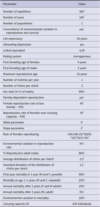
The analysis was performed in six steps: (1) we developed scenarios in which only the initial population values were changed to verify the MVP of the species; (2) we created a base scenario from the MVP, in which we assumed that the population is not affected by any external factor, being considered an “ideal” population; (3) we simulated scenarios by changing the value of parameters to perform the sensitivity analysis, identifying parameters which could affect the result of the simulation; (4) we modelled different changes that can occur in the landscape, such as decrease or increase in habitat; (5) we estimated the impacts of catastrophes and external threats, such as hunting and trafficking; (6) finally, we simulated the effect of introducing individuals from captivity into the population. The data used in the construction of the scenarios in VORTEX are shown in Table 1.
Input values and parameters used in creating the population model of Spix’s Macaw Cyanopsitta spixii.

1 Authors’ source 2022.
2 Based on 2020 Spix’s Macaw captivity programme monitoring report.
3 According to Lacy et al. Reference Lacy, Miller and Traylor-Holzer2021.
a Formula generated by VORTEX from the inclusion of density-dependent reproduction data.
Negative exponential nonlinear scaling between density estimates and body mass of Psittaciformes native to the region, with expected density prediction for Spix’s Macaw Cyanopsitta spixii. Dots in black indicate the species with density estimates, the black dashed line indicates the fitted nonlinear model (density ~beta1*massabeta2; beta 1 = 0.013, beta 2 = 0.0013), and the blue dot indicates the expected value for Spix’s Macaw (estimated weight 300 g).

Population density
The population density of Spix’s Macaw was estimated from the density of other psittacines found in the release area: Primolius maracana (0.009 individuals/ha, weight = 256 g), Thectocercus acuticaudatus (0.009 individuals/ha, weight = 171 g), Eupsittula cactorum (0.013 individuals/ha, weight = 70 g), and Amazona aestiva (0.008 individuals/ha, weight = 451 g) (Silva Reference Silva2016). These estimates were performed using linear transects (Silva Reference Silva2016), modelled in the DISTANCE program. Since vertebrate population density typically scales allometrically with body mass (Silva and Downing Reference Silva and Downing1995), a negative exponential nonlinear regression was fitted to then predict the expected density for Spix´s Macaw, considering a body mass of 300 g (Barros et al. Reference Barros, Soye, Miyaki, Watson, Crosta and Lugarini2012).
Carrying capacity (K)
The carrying capacity was calculated based on the size of the Spix’s Macaw protected areas (Gov.Br. 2018). This density was adjusted based on the records provided by the ICMBio monitoring team of the last free-living male and habitat selection based on the area used by the birds after release. In addition, we considered the result of the spatial analysis performed in RangeShiftR.
MVP and initial population size
To verify the MVP, simulations were run with initial population size (N) the only value changed between scenarios. The scenarios had N varying between 15, 20, 50, 100, and 200 individuals. We analysed which population scenario had the lowest PE, as well as the scenario that presented the lowest number of individuals, this being the minimum size required for the population to persist. The resulting MVP was used in the construction of the baseline scenario. In this scenario, we assumed that the population is not affected by any external factors, resulting in an ideal population.
Sensitivity analysis
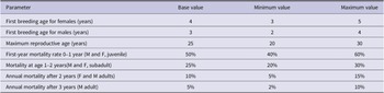
This analysis seeks to identify which input parameters are sensitive, i.e. which can alter the population dynamics and, consequently, the results of the simulations (Pe’er et al. Reference Pe’er, Matsinos, Johst, Franz, Turlure, Radchuk and Malinowska2013). It is used mainly when working with species on which few data are available. Thus, we tested the effect of changing specific parameters as described in Table 2.
Parameters and values used in the sensitivity analysis.

Threats: catastrophes, removals, and habitat loss
Catastrophes are extreme cases that can impact different species. We modelled the effect of two types of catastrophe on the population, i.e. diseases and severe drought. Psittaciformes are prone to diseases such as avian bornavirus that affects the central nervous system and is associated with the development of the incurable proventricular dilatation disease (Staeheli et al. Reference Staeheli, Rinder and Kaspers2010). Droughts can directly affect local populations by impairing the availability of resources such as water and food. We also deal with the existence of inbreeding, since the individuals studied are related to each other, which increases the cases of infertility and hatching failure (Barros et al. Reference Barros, Soye, Miyaki, Watson, Crosta and Lugarini2012).
To gauge the impact of disasters, VORTEX allows researchers to specify what is the chance of occurrence of these events and what impact will they have on the reproduction and survival of individuals (Table 3). The program infers that severity is a proportion of the values recorded in years when no catastrophes occur (Lacy et al. Reference Lacy, Miller and Traylor-Holzer2021).
Types of disasters and their impact values as per VORTEX software standards.

1 Authors’ source 2022.
Spix’s Macaw is subject to predation (White et al. Reference White, Collar, Moorhouse, Sanz, Stolen and Brightsmith2012, Reference White, Collazo, Dinsmore, Llerandi-Román and Devore2014, Reference White, Abreu, Benitez, Jhonson, Lopez, Ramirez and Rodriguez2021), hunting, and extraction for illegal trade (Barros et al. Reference Barros, Soye, Miyaki, Watson, Crosta and Lugarini2012). The effects of these removals were evaluated by VORTEX, based on an annual removal of five individuals, regardless of inter-sexual differences, over a simulated period of 100 years.
Habitat loss has been one of the recurring reasons for the extinction of the species in the wild (Barros et al. Reference Barros, Soye, Miyaki, Watson, Crosta and Lugarini2012, Gomides et al. Reference Gomides, Machado, Evangelista‐Vale, Martins‐Oliveira, Pires‐Oliveira, Muller and da Rosa2021). With this concern, we simulated the reduction and increase of K, verifying the influence of this parameter on the persistence of the population. The influence of habitat size on K was verified by simulating three scenarios: (1) with a 5% annual decrease in K for 10 years; (2) a 10% annual decrease in K for 10 years; (3) a 10% annual increase in K for 10 years.
Supplementation of individuals
The Spix’s Macaw reintroduction project aims to release additional individuals from the captive population annually. To test the need for this action, we simulated that 10–30 individuals would be supplemented annually into the population and that the supplementation would take place over 10, 20, and 30 years.
RangeShiftR (spatial evaluation)
For spatially explicit analyses, we used the RangeShiftR platform, made available in the R programming language (Malchow et al. Reference Malchow, Bocedi, Palmer, Travis and Zurell2021). We used the same parameters applied in the simulations performed with the VORTEX software (see above).
The geographical bases used were provided by the Ecology and Environmental Monitoring Center (Nema) of the Federal University of São Francisco Valley (Univasf), and 33 classes were included that considered the vegetational size of the caatinga and types of geological formation. For this modelling we aggregated these classes into four categories focused on the vegetation sizes of the caatinga: (1) sparse open; (2) open woody; (3) dense shrub; (4) tree. A restoration map prepared by Nema was also used, indicating the locations and targets of shrub and tree areas to be restored.
For emigration, it was assumed that differences occur between sexes (where males are more likely to emigrate), ages (where emigration only occurs in the pre-reproductive year and the first reproductive year), and that there is strong density-dependence in emigration. The probabilities of emigration follow Table 4, in which the age of pre-reproductive dispersal and the highest propensity of males to disperse are observed. Strong density-dependence on emigration was assumed because this was a release event in a landscape with local extinction.
Assumed emigration probabilities across ages and between genders.

We used the post-release locations of 10 individuals (eight Spix´s Macaws and two Blue-winged Macaws), as well as the locations of the last Spix’s Macaw recorded in the wild to access the utilised area, dispersal probability, and habitat selection of these individuals. The locations of each individual were estimated by triangulating the azimuths taken by radiotelemetry.
After having the locations projected, the area used by each individual was estimated using the minimum convex polygon method, considering 95% of the locations (MCP95%) (Worton Reference Worton1989). Using only 95% of the locations proved to be conservative since few locations were observed, and the locations were estimated using only two azimuths, which generated large unaccounted triangulation errors. The Mean Square Shift (MSD) method was also used to access the dispersion pattern of the birds with respect to the release point (Bastille-Rousseau et al. Reference Bastille-Rousseau, Potts, Yackulic, Frair, Ellington and Blake2016, Oliveira-Santos et al. Reference Oliveira-Santos, Moore, Severud, Forester, Isaac, Chenaux-Ibrahim and Garwood2021). Finally, a second-order Resource Selection Function (RSF) was used to access habitat selection of individuals (Johnson Reference Johnson1980, Oliveira-Santos et al. Reference Oliveira-Santos, Moore, Severud, Forester, Isaac, Chenaux-Ibrahim and Garwood2021)
Two continuous maps were created characterising the habitats hypothesised to be preferred by the species, i.e. drainage areas (i.e. rivers) and areas with shrub and tree vegetation. To characterise habitat availability in the landscape, a single MCP100% area containing all individual locations was estimated, and then 100 locations were randomly drawn for each individual to represent habitat availability in the release area.
The distance from each random location to the nearest shrubby or arboreal vegetation, and drainage was measured. These available locations were coded as 0s. After this the habitat used was also measured, by calculating the distance from each observed location of an individual to the nearest shrubby or woody vegetation, and drainage area. The locations observed (used) by the birds were coded as 1s. This system of used (1s) and available (0s) habitats could be solved through a conditional logistic regression (CLR), where the model is conditioned for each individual, thus considering individual heterogeneity. The solution of this CLR then allowed the estimation of a selection of areas used based on preferences for areas with different distances to shrubby vegetation and drainage sites. Based on habitat preference and specific density, we calculated that riparian vegetation is required for Spix’s Macaw over the years.
Results
We assume that a population is viable, i.e. has the ability to persist for a given time, when presenting a PE of less than 5%. Based on this, we analysed the modelled scenarios, testing the variables discussed in the previous section.
Population density
Using the fitted model, a prediction could be made for a 300 g psittacid, predicting an overall density of 0.009 individuals/ha for a psittacid of the size of Spix’s Macaw (Figure 1), with a good fit of the negative exponential model in the allometric density relationship (model density ~0.013*mass0.0013; R² = 0.72).
Land use, land cover, and carrying capacity (K)
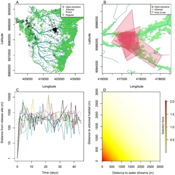
An average of 33 (1–50) locations per individual was obtained, where recently released individuals had an average area of use of 143 ha (51–209 ha), which corresponds to a small portion of the area used by the last monitored Spix’s Macaw in the wild (2,800 ha) (Figure 2a). Overall, the birds were extremely cohesive at the post-release time, having overlapping areas of movement (Figure 2b). According to the net-squared displacement (NSD), the birds also appear to be anchored in daily movements ranging from 100 m to 1,000 m from the release site, and at times reaching almost 10 km away (Figure 2c). Also, when solving the CLR, a strong selection was found for areas near shrubby or arboreal habitat (β = -0.001, P <0.05) and drainage areas (β = -0.003, P <0.05). Therefore, unattached individuals adjusted their use areas preferentially to locations near riparian forests, with a very low probability of occupying areas with distances greater than 1 km from both arboreal areas and streams simultaneously (Figure 2d).
(A) Distribution of locations for reintroduced individuals. Note that the locations on the left of the map correspond to the last monitored native Spix’s Macaw Cyanopsitta spixii. (B) MCP95% polygons representing the area used by individuals after release. (C) Curves observed by the Mean Squared Shift method relative to the release point. (D) Second-order habitat selection estimated to verify habitat preferences for allocation of used areas.

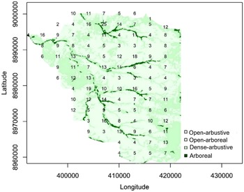
Projected density information, the area the birds used after release, and the habitat selection of the last monitored Spix’s Macaw in the wild were used to define the carrying capacity per habitat. An overall density estimate of 0.009 individuals/ha was then assumed, which would need to be adjusted for each habitat. The habitat selection ratio (use/available) for the last Spix’s Macaw indicated that tree habitat was used about five times more than available; shrub habitat was used at a ratio of 0.5 to available; open woody habitat was used at a ratio of 0.1 to available; open habitat was never used. We therefore used these selection ratios to multiply the overall density and thus adjust the densities by habitat type: sparse open = 0 (no habitat); woody open = 0.0009 individuals/ha; dense shrub = 0.0044 individuals/ha; arboreal = 0.044 individuals/ha. To check the viability of these values, we ascertained the area used by the 10 released individuals, which appear to be cohesive (using overlapping areas), and covers about 356 ha, would generate a current local density of 0.028 individuals/ha (10 individuals/356 ha). Note that the release site is located in an area with a dominance of favourable habitats, i.e. large cover of shrub and tree vegetation at the riverside. When projecting the overall landscape abundance (K) by weighing habitat availability (i.e. the carrying capacity of the modelled map), it is expected that up to 870 individuals could be sustained in the region (total area ~189,000 ha) (Figure 3). This value would be five times higher if we consider the map with all restored regions (K = 4,500 individuals).
Carrying capacity estimated by patch and environment to guide future releases at new sites. The sum totals the expected carrying capacity for the entire landscape (K = 870 individuals of Spix’s Macaw Cyanopsitta spixii).

MVP and base case
The results indicated that an initial population of 20 individuals has a PE of less than 1% (0.004) within 100 years. Therefore, this was assumed to be the minimum viable size of individuals needed to have a stable population. Thus, 20 individuals were adopted as the initial population size in all scenarios subsequently modelled. We adopted this model as the baseline scenario (Figure 4).
Average population size obtained from the base case simulations. The dashed line represents the estimated carrying capacity of 870 and the solid line the population growth projection.

According to the VORTEX results (Table 5), the average population size for the baseline scenario at the end of 100 years was 824.29 (standard deviation [SD] = 124.22). The determined growth rate, which does not consider stochastic fluctuations, inbreeding depression, and immigration/emigration, was 0.1076, representing a potential growth rate of about 11% per year. The average stochastic growth rate was 0.0542 when random events occur.
Results of the identification of the minimum viable population of Spix’s Macaw in the area of interest. Rdet = determined growth rate; Rstoch = stochastic growth rate; PE = probability of extinction; Nall = mean population size; GD = genetic diversity. Standard deviation of the variables is given in parentheses.

Sensitivity analysis
Sensitivity analysis explored parameter uncertainties, indicating data which may need further research. The most sensitive parameters of the model were chick mortality (0–1 year of age) and male mortality from 3 years of age onwards (Figure 5).
Parameters used in the sensitivity analysis and the smallest and largest values comparing the stochastic growth rate between them. The horizontal line at 5% represents the Rstoch of the base case. FRF = first reproductive age for females; FRM = first reproductive age for males; MAR = maximum age for reproduction; Mort_0–1 = first year mortality 0– 1 year (M and F, juvenile); Mort_1–2 = mortality at age 1–2 years (M and F, subadult); MortF_2 = mortality after age 2 years for females; MortM_2 = mortality after age 2 years for males; MortM_3 = mortality after age 3 years (M, adult).

Threats
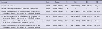
The exclusive presence of catastrophes in the baseline scenario did not prove to be a major threat to the persistence of the population. In this scenario, the PE of the species was 3%, thus having a viable population (Table 6, scenario a). However, it resulted in a reduction of about 13% in population size (Figure 6).
Effects of catastrophes, threats, and supplementation on the simulated population. Rdet = determined growth rate; Rstoch = stochastic growth rate; PE = probability of extinction; Nall = mean population size; GD = genetic diversity; AE = estimate of the year when the population reaches stability. Standard deviation of the variables appears in parentheses.

Influence of catastrophes (disease and severe drought) on the average population size of Spix’s Macaw Cyanopsitta spixii over 100 years. The solid line represents the baseline scenario and the dashed line is the projected population growth in the scenario with catastrophes.

In nature, species are susceptible to the removal of individuals caused by external influences, e.g. predation (White et al. Reference White, Collar, Moorhouse, Sanz, Stolen and Brightsmith2012, Reference White, Collazo, Dinsmore, Llerandi-Román and Devore2014, Reference White, Abreu, Benitez, Jhonson, Lopez, Ramirez and Rodriguez2021) and power line electrocution (Biasotto et al. Reference Biasotto, Pacifico, Paschotto, Filadelfo, Couto, Sousa and Mantovani2022). To get a more realistic view, we simulated the combined action of catastrophes and the annual removal of five individuals: this resulted in a 100% PE in 100 years (Table 6, scenario b). Furthermore, the stochastic growth rate was negative (-0.0539; SD = 0.1224), indicating that the species has no growth potential within these environmental circumstances.
We found that if the population loses 5% of its habitat annually over a 10-year period, it will remain viable (PE = 0.018). However, the average population size will drop from 824 to 410 individuals (SD = 75.26) (Figure 7). If this habitat loss is 10%, the population will go extinct within an average time of 11 years, with a probability of 100%. If there is a 10% annual increase in habitat, and consequently K, the probability of extinction will be 1% (0.014), with an average population size of 1,592 individuals (1,592.18, SD = 360.44).
Average population size of Spix’s Macaw Cyanopsitta spixii, demonstrating variation in carrying capacity over 100 years compared with the baseline scenario. I10 = 10% annual increase in K over 10 years; D10 = 10% annual decrease in K over 10 years; D5 = 5% annual decrease in K over 10 years.

Population supplementation
The analysis indicates that one method to overcome these threats would be to assist the population by releasing individuals, i.e. supplementation. Even in the scenarios with the effect of drought, disease, and hunting, supplementing individuals aided in the recovery of the population. All simulations indicating the release of 20–30 individuals over 5–20 years showed a positive stochastic growth rate, with 100% probability of persistence over 100 years (Table 6, scenarios c, d, e, and f). The average population size in these four scenarios resulted in about 848 individuals, which is higher than the value found in the baseline scenario (mean population size = 824.29), in which there are no threats (Figure 8). Since the simulations and results are based on random sampling, the population will tend to fluctuate, i.e. the simulated population will not be completely stable. However, we found that releasing individuals contributes to how quickly the population reaches carrying capacity (Figure 5), which may portray the optimal state of the species.
Comparing mean population sizes before the effect of the presence of threats, compared with the effect of releasing individuals into the population. Baseline = scenario with baseline data, no effect of threats and catastrophes; CH = scenario with presence of catastrophes and annual removal of five individuals; CHS = scenario with presence of catastrophes, annual removal of five individuals, and supplementation of 20 individuals for 20 years.

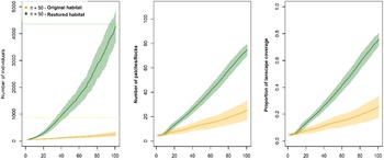
Reforesting the riparian tree areas would greatly increase the carrying capacity of the landscape (~4,500 individuals), accelerating population growth, and thus the final numbers (near carrying capacity), number of patches/flocks (~75 flocks), and landscape coverage would reach almost 80% in 100 years (Figure 9).
Population trajectory, number of patches/flocks, and area occupied in simulations over 100 years for 50 individuals released in the original landscape or in the restored landscape. The yellow dashed line in the graph on the right corresponds to the carrying capacity of the original landscape, and the green dashed line is the restored landscape.

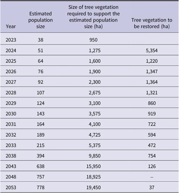
The carrying capacity of habitat is limited to the current 4,497 ha of riparian vegetation, which must be reforested to achieve almost 20,000 ha (Table 7). It means that it is necessary to reforest at least 15,000 ha in the following years to maintain the carrying capacity of the habitat for the growing population of Spix’s Macaw.
Size of tree vegetation required to sustain the estimated population size per year.

Spatial projections
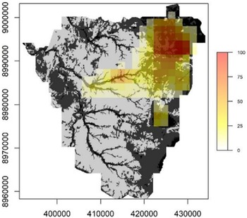
It was also possible to predict the direction and speed of occupation of the landscape with population growth. Considering the preferred habitats, emigration rates, and dispersal resistance employed in the model, we observed the expectation of a main east–west flow of birds, and a slower flow in the riparian areas in a north-west–south-east direction (Figure 10).
Kernel density of the dispersal trajectories of the emigrants generated by the model in which 50 individuals were released at the original release site. The warmest values correspond to the sites with the highest fate of dispersers.

Discussion
The present study is an ex-ante analysis that used the best available information to model future scenarios. Considering that this is a species with limited information on its biology and ecology in the wild (Barros et al. Reference Barros, Soye, Miyaki, Watson, Crosta and Lugarini2012), we made inferences based on information from a captive population, from species with a similar biology, and from the experience of specialists. Thus, the results presented here will need to be regularly revisited to increase their accuracy as new information becomes available. Thus, the input values can serve as a starting point for future research.
Even with this limitation, our findings should be factored into release planning and in situ management actions. The data on land use and occupation by the reintroduced birds allowed us to confirm the pattern recorded in the literature on the species (Juniper and Yamashita Reference Juniper and Yamashita1991, Juniper Reference Juniper2002, Barros et al. Reference Barros, Soye, Miyaki, Watson, Crosta and Lugarini2012, Cavalcanti et al. Reference Cavalcanti, Rafael, Barbosa, Braz and Ribeiro2020), with respect to its preference for arboreal habitat near waterways. Thus, the estimated population density of 0.009 individuals/ha was stratified according to landscape use, showing a higher density of 0.04 individuals/ha in the arboreal vegetation area. This allowed us to estimate the carrying capacity of the environment, which conservatively stood at 870 individuals for the two protected areas.
From the carrying capacity of the environment and the biological and ecological parameters of Spix’s Macaw, the base scenario was defined and simulations were performed. The MVP of Spix’s Macaw is 20 mature individuals. The constructed base case scenario points to a growth rate of 11% per year with an estimate of reaching 824 individuals (SD = 124) in 100 years. However, the simulations indicate that the mortality of nestlings and males from three years of age, aggravated by catastrophes and removal of individuals, would lead to the extinction of the species.
The continuous supplementation of novel individuals into the population would likely help to stabilise the population and minimise the expected fluctuations, once some of the threats can, at most, be mitigated but not prevented. So, the perpetuation of the species in the wild depends on the supplementation of the population. The best outcome scenario suggests the introduction of 20 individuals per year over the next 20 years and the adoption of mitigating measures that avoid mortality in the early life stages of these birds. In this scenario the population size will be close to an average population size of 849 individuals (N = 849.05 ± 46.26), being reached by 30 years. Furthermore, this scenario resulted in an annual stochastic growth of 10% (stochastic r = 0.0982 ± 0.1161), considering random demographic and environmental events. Furthermore, the supplemented population would reach carrying capacity three times faster (~25 years) than the non-supplemented base population (~100 years). The need for continued supplementation imposes the need to maintain ex situ management of Spix’s Macaws at a high standard of performance.
In the first release, the main threat faced by Spix’s Macaw was predation by raptors (authors’ information) as noticed in other conservation psittacine programmes (White et al. Reference White, Collar, Moorhouse, Sanz, Stolen and Brightsmith2012, Reference White, Collazo, Dinsmore, Llerandi-Román and Devore2014). The dispersive individuals or pairs were more prone to be predated. Furthermore, the methodologies that mitigate excessive or premature dispersion from the release area of the population might increase the survival of released Spix’s Macaws favouring prompt breeding and decreased mortality in the early life stages of these birds and the consequent re-establishment of the species. The soft release of captive-reared parrots on-site at a captive breeding facility (White et al. Reference White, Abreu, Benitez, Jhonson, Lopez, Ramirez and Rodriguez2021) will promote survival, site fidelity, flock cohesion, and prompt reproduction by released Spix’s Macaws and might also help the establishment of the population in the area. Heterospecific groups with native Blue-winged Macaws favour the acclimation of the first group to the release area and lead with the low number of individuals in the population. The presence of a large number of conspecifics with newly released Spix’s Macaws and a captive breeding population in the release site are two other actions to be taken to avoid mortality after release and mitigate or reduce per capita risk associated with a potential predator (see White et al. Reference White, Abreu, Benitez, Jhonson, Lopez, Ramirez and Rodriguez2021). Artificial nests in the release area can be used to assist Spix’s Macaw to help avoid mortality of chicks (Brightsmith Reference Brightsmith2005), and promote site fidelity. The management of natural nests or nest boxes can be enhanced by minimising snake predation through the use of metal belts around the base of the nest tree and ensuring there is no contact between its canopy and those of its neighbours (Vilarta et al. Reference Vilarta, Wittkoff, Lobato, Oliveira, Pereira and Silveira2021).
Habitat condition was another factor evaluated. For the baseline scenario we found that the population would be viable even with a 5% habitat reduction. However, 10% habitat loss would generate an absolute risk of extinction after 11 years of release. Restoring 10% of the habitat, on the other hand, would generate a persistent final population. If the 20-year population supplementation scenario is adopted, habitat will need to be restored to support the expected population growth. Restoration of the areas will also provide acceleration of population growth by avoiding competition and still sustain a stable population for 100 years. The planning of restoration actions for riparian forests should occur in the east–west and north-west–south-east direction, according to the projected population expansion.
Conclusions
The findings presented here are elements that should be observed in the development of the Spix’s Macaw reintroduction programme. According to our results, the initial population of Spix’s Macaw to be reintroduced should be 20 mature individuals, which is the size of a MVP. The reintroduction technique should consider the mitigation of breeding males and mortality in the early life stages of parent-reared wild chicks.
Catastrophes do not contribute significantly to a higher extinction risk in the population, but threat factors like the removal of individuals from the wild and the mortality of young birds and three-year-old males increase the likelihood of extinction to 100%. Similarly, the loss of 10% of the habitat will also lead to the extinction of the species within 11 years. Therefore, the excessive and premature dispersal of the release area should be avoided for predation mitigation or other threats such as poaching or power line electrocution. Even if predation is a permanent threat, predator control measures might be performed.
According to the simulations performed, the best scenario for the fastest establishment of a stable population of Spix’s Macaw is one in which the initial population of 20 individuals will be supplemented annually over the following 20 years. This is essential while maintaining preventative measures to minimise the likelihood of catastrophes, individual removals from the wild, and mortality in juveniles and males up to three years old, as well as habitat loss.
We recommend facilitating and establishing conservative actions towards successive habitat restoration, especially of riparian forests, to further accelerate population growth by increasing the carrying capacity of the environment, since the Spix’s Macaw population will expand its area of occupation over time according to its growth.
Considering the need for supplementation of individuals over the next 20 years, the Spix’s Macaw captive programme needs to be maintained and strengthened.
Finally, considering the initial comments regarding the gaps in information identified in the analyses carried out and the expansion of knowledge from the release of the birds, we suggest that a continuous monitoring programme of the reintroduced birds be established, and that the novel information collected be applied to review the scenarios carried out here.
Acknowledgements
We thank the organisations involved in the Spix’s Macaw captive programme and Action Plan, the reviewers who helped improve this article, and the Curaçá community and project field team.