1. Introduction
When a granular system is subjected to flow or vibration, separation of its components occurs, resulting in spatially distinct regions. This phenomenon, known as segregation, is a key challenge in many solid-handling industries such as pharmaceutical, food processing, ceramic, metallurgical and steel industries. Segregation also occurs in geophysical situations such as debris flows, snow avalanches, landslides, rock falls etc. Although surface properties and particle shapes can also cause segregation of granular materials, the differences in particle sizes and/or densities are the primary factors that lead to the segregation. A large body of literature reporting the segregation of granular mixtures through experimental observations (Gray & Hutter Reference Gray and Hutter1997; Hsiau & Chen Reference Hsiau and Chen2002; Jain, Ottino & Lueptow Reference Jain, Ottino and Lueptow2005; Yang Reference Yang2006; Jha & Puri Reference Jha and Puri2010; Asachi et al. Reference Asachi, Hassanpour, Ghadiri and Bayly2018; Liao Reference Liao2019; Liao & Tsai Reference Liao and Tsai2020; Rodolfo et al. Reference Rodolfo, Rondinelli, Raphael, Claudio and Marcos A.S.2020; Pillitteri et al. Reference Pillitteri, Opsomer, Lumay and Vandewalle2020) and discrete element method (DEM) simulations (Pereira et al. Reference Pereira, Pucilowski, Liffman and Cleary2011a,Reference Pereira, Sinnott, Cleary, Liffman, Metcalfe and Šutalob; Chand et al. Reference Chand, Khaskheli, Qadir, Ge and Shi2012; Combarros et al. Reference Combarros, Feise, Zetzener and Kwade2014; Ayeni et al. Reference Ayeni, Wu, Joshi and Nandakumar2015; Lim Reference Lim2016; Pereira & Cleary Reference Pereira and Cleary2017; Qiao et al. Reference Qiao, Duan, Dong, Wang, Jiang, Zhu and Zhao2021) is available. However, these studies largely focus on reporting the observations for the segregating mixtures and lack theoretical formulation for predicting segregation.
A theoretical approach for modelling granular segregation based on the kinetic theory of granular mixtures has been proposed decades ago (Jenkins & Richman Reference Jenkins and Richman1985; Savage & Lun Reference Savage and Lun1988). Significant progress has been made in the last few decades to extend these models for dense granular flows (Larcher & Jenkins 2013, 2015; Kumaran Reference Kumaran2008; Larcher & Jenkins Reference Larcher and Jenkins2013, Reference Larcher and Jenkins2015; Jenkins & Larcher Reference Jenkins and Larcher2020). Larcher & Jenkins (Reference Larcher and Jenkins2013) developed a kinetic theory to describe binary size and density segregation in dense granular flows and predicted the steady-state concentration of species. These predictions, when compared with the DEM data from the study by Tripathi & Khakhar (Reference Tripathi and Khakhar2011), showed reasonable agreement with different density mixtures for chute flows at low inclinations. However, significant deviations were observed at larger inclinations. In addition, significant deviations were observable for different size mixtures as well. Larcher & Jenkins (Reference Larcher and Jenkins2015) extended this work to predict the time evolution of segregation and their predictions showed qualitative agreement with the DEM data of Thornton et al. (Reference Thornton, Weinhart, Luding and Bokhove2012) as well as that from the experimental results of Savage & Lun (Reference Savage and Lun1988).
Gray and coworkers (Gray & Ancey Reference Gray and Ancey2011, Reference Gray and Ancey2015; Gray & Chugunov Reference Gray and Chugunov2006; Gray & Ancey Reference Gray and Ancey2011, Reference Gray and Ancey2015; Gray Reference Gray2018) developed a theoretical framework to study the phenomena of segregation in free surface flows. In this approach, the advection–diffusion–segregation equation for each mixture species is solved to predict the segregation. The knowledge of the flow kinematics, segregation model and diffusion coefficient is required to be able to predict the segregation. An empirical segregation model for different size binary granular mixtures was proposed by Fan et al. (Reference Fan, Schlick, Umbanhowar, Ottino and Lueptow2014) and Schlick et al. (Reference Schlick, Fan, Umbanhowar, Ottino and Lueptow2015), who used this framework to predict the segregation in heap and rotating cylinders by imposing the flow kinematics from the simulations/experiments. This segregation model was extended by Schlick et al. (Reference Schlick, Isner, Freireich, Fan, Umbanhowar, Ottino and Lueptow2016) to accommodate polydisperse mixtures and was shown to be in qualitative agreement with DEM simulations. A similar approach was used to account for the combined effect of size and density segregation as well by Duan et al. (Reference Duan, Umbanhowar, Ottino and Lueptow2021, Reference Duan, Peckham, Umbanhowar, Ottino and Lueptow2023).
Relatively fewer studies have focused on segregation solely due to density differences. Xiao et al. (Reference Xiao, Umbanhowar, Ottino and Lueptow2016) studied density segregation of binary granular mixtures in heap flow using both experiments and DEM simulations. The authors proposed a linear empirical segregation model based on their DEM data and solved the convection–diffusion–segregation equation by incorporating the flow kinematics from the DEM data. Notably, the theoretical predictions were in good agreement with DEM data at steady state. Fry et al. (Reference Fry, Umbanhowar, Ottino and Lueptow2018) modified the linear empirical model to account for the effect of pressure for size as well as density segregation of binary mixtures in the case of plane shear flow. Using this model, Fry et al. (Reference Fry, Umbanhowar, Ottino and Lueptow2019) predicted steady-state concentration profiles that were found to be in good agreement with DEM data for a  $50\,\% {-} 50\,\%$ mixture of different density grains in plane shear.
Deng et al. (Reference Deng, Umbanhowar, Ottino and Lueptow2018) generalised the segregation model for different density binary mixtures to multicomponent mixtures differing in density. Following the previous studies, the authors used the velocity profiles obtained from DEM simulations to predict the evolution of segregation with time. This essential requirement of the knowledge of flow kinematics at each instant can be avoided by solving the momentum balance equations using the granular rheology and intercoupling this with the advection–diffusion–segregation equation. This enhances the predictive capability of these approaches to systems where the flow kinematics may not be easy to measure.
Such an approach has been followed by Barker et al. (Reference Barker, Rauter, Maguire, Johnson and Gray2021) who implemented a three-dimensional (3-D) continuum model to predict the size segregation for multicomponent mixtures in free surface flows. The model was successfully able to predict qualitative behaviour in flow geometries such as chute flow and rotating cylinder flow. This continuum model has recently been used to predict the size segregation in a triangular rotating drum as well (Maguire et al. Reference Maguire, Barker, Rauter, Johnson and Gray2024). While Barker et al. (Reference Barker, Rauter, Maguire, Johnson and Gray2021) use the segregation model of Trewhela, Ancey & Gray (Reference Trewhela, Ancey and Gray2021),Yang et al. (Reference Yang, Zheng, Bai and Yu2021) use the empirical segregation model of Gajjar & Gray (Reference Gajjar and Gray2014) to predict transient size segregation in a periodic shear cell, chute flow and rotating drum. The predictions from the model were compared with DEM data and found to be in good agreement. Recently Trewhela (Reference Trewhela2024) have used the segregation model of Trewhela et al. (Reference Trewhela, Ancey and Gray2021) along with the regularised  $\mu {-}I$ rheology proposed by Barker et al. (Reference Barker, Schaeffer, Shearer and Gray2017) to predict the time-dependent size segregation in a plane shear flow using a one-dimensional (1-D) continuum model. Liu, Singh & Henann (Reference Liu, Singh and Henann2023) have coupled the size segregation model for binary mixtures which accounts for the shear-strain-rate-gradient-driven segregation with a non-local rheological model for granular flows to successfully predict the segregation in vertical and annular shear flows. This model has been extended by Singh, Liu & Henann (Reference Singh, Liu and Henann2024) to account for pressure-gradient-driven segregation as well, and the predictions from the model agree well with DEM simulations for chute flows and plane shear flows.
Transient segregation of granular mixtures differing in density has been studied by Tirapelle et al. (Reference Tirapelle, Santomaso, Richard and Artoni2021). The authors predicted time-dependent behaviour of a binary mixture of different density particles using a segregation model based on the particle force-based theory. While the authors partially attempted to couple the rheology with the segregation model, they did not solve the momentum balance equations and used the flow kinematics obtained from the DEM simulations. The authors performed experiments in an annular cylinder in which the front and the back wall effects also play an important role along with the confinement at the top surface through which pressure was exerted on the material. They used an initial configuration where the light species was concentrated near the base. While the density ratios used in experiments ranged from  $1.4$ to
 $8.25$, the theoretical predictions of the model were compared with experimental data only up to density ratios of
 $3.7$. A careful look at their results shows that the continuum simulations reported by the authors fail to qualitatively capture the concentration variation in an equal composition mixture even for low density ratios of
 $1.4$ and
 $2.59$.
Segregation of different density mixtures by accounting for the intercoupling of the rheology and segregation was first studied by Tripathi & Khakhar (Reference Tripathi and Khakhar2013). The authors derived a particle force-based model to predict the segregation of a binary mixture of different density particles in periodic chute flow at steady state. This segregation model has been generalised for a multicomponent density mixture by Sahu et al. (Reference Sahu, Kumawat, Agrawal and Tripathi2023). This particle force-based model stands out as the most promising segregation model for different density mixtures. The model does not require any empirically fitted parameter and is able to predict the steady-state segregation of multicomponent mixtures for a wide range of density ratios, inclination angles and compositions of the species.
In this work, we study the time-dependent behaviour of flow and segregation of granular mixtures, and explore the applicability of this particle force-based model to accurately predict the time-dependent evolution of segregation along with other flow properties. We simultaneously solve the momentum balance equations by using  $\mu {-}I$ rheology along with the segregation–diffusion equation. Due to the periodic simulation box used in DEM simulations, we consider the variation of the flow properties only along the vertical direction, and ignore the variations along the flow and vorticity directions. We perform DEM simulations of binary and ternary mixtures differing in density for different mixture compositions and density ratios at two different inclination angles. In addition, we explore the applicability of the proposed theoretical approach for different initial configurations of the species. Specifically, we consider the evolution of segregation for an initially well-mixed configuration along with two almost completely segregated configurations of light species near the base and heavy species near the base. The results presented in this work show that transient segregation in a periodic chute can be very well captured by our 1-D continuum model for binary, ternary and quaternary mixtures for well-mixed and heavy-near-base configurations. However, the model predictions do not agree with DEM simulation results for the light-near-base initial configuration. More importantly, the failure of the 1-D model for a short time duration for this configuration reveals the occurrence of an instability-driven, quick segregation phenomenon that has received little attention in the literature.
The organisation of the paper is as follows. DEM simulation methodology is summarised in § 2. The continuum model comprising the time-dependent momentum balance and convection–diffusion equations inter-coupled with particle force-based segregation model and granular mixture rheology are detailed in § 3. We report the time-dependent properties for the case of initially well-mixed configuration for binary mixtures in § 4 along with a comparison of our results with the kinetic theory model of Larcher & Jenkins (Reference Larcher and Jenkins2015). The results of multicomponent mixtures for the well-mixed case are discussed in § 5. Section 6 presents the results for heavy-near-base and light-near-base initial configurations. We report the presence of Rayleigh–Taylor-like instability in different density granular mixture flows in § 7 and provide a summary of our findings in § 8.
2. DEM simulation methodology
DEM simulation snapshots for equal composition mixture flowing over an inclined plane at an inclination angle of  $\theta$. (a) Binary mixture having density ratio
 $\rho _H/\rho _L = 3.0$ and (b) ternary mixture having
 $\rho _H: \rho _M : \rho _L$ =
 $3:2:1$. Green, red and blue particles represent the heavy-, medium- and low-density particles, respectively. Black particles represent the rough bumpy base of thickness
 $1.2d$. The orange arrow indicates the direction of flow.

We perform simulations of spherical particles of identical sizes (diameter  $d$) and different densities flowing over an inclined plane using DEM. The particles are assumed to be frictional and slightly inelastic. The inter-particle coefficient of normal restitution is
 $e = 0.88$ and the inter-particle friction coefficient of
 $\mu _{pp} = 0.5$ is used in all the simulations. We consider a simulation box that spans an area of
 $20d \times 20d$ in the streamwise (
 $x$) and vorticity (
 $z$) directions. A periodic boundary condition is imposed along the streamwise direction. To avoid shearing along the vorticity direction, we use a periodic boundary in the
 $z$ direction as well. Use of the periodic boundaries in the
 $x$ and
 $z$ directions facilitates detailed quantitative comparison of DEM simulation results with continuum model predictions of unidirectional density segregation. The height of the simulation box in the
 $y$ direction is
 $40d$ and a total of
 $10\, 000$ particles are used in the simulation. At the start of the simulation, particles are generated in a cubic lattice so that two adjacent particles are not in contact. The particles are settled at inclination angle
 $\theta = 0^\circ$ under the influence of gravity until the average kinetic energy of particles in the layer becomes less than
 $10^{-6} mgd$. The layer height after settling the particles turns out to be approximately
 $24d$. The inclination angle is then increased to the desired value so that particles start to flow. The simulation is performed for a sufficiently large time so that all the properties of interest achieve a steady value. This time duration ranges from
 $3000$ to
 $6000$ dimensionless time units. We employ the linear spring and dashpot model to calculate contact forces in both the normal and tangential directions. The normal and tangential spring stiffness is
 $k_{n} = 2 \times 10^{5}$
 $mg\,d^-{^1}$ and
 $k_{t} = 2k_{n}/7$, respectively. Further information regarding the contact force model can be found from Tripathi & Khakhar (Reference Tripathi and Khakhar2011).
DEM snapshots for equal composition binary as well as ternary mixture, are shown in figures 1(a) and 1(b). Green, red and blue particles represent the heavy-, medium- and low-density particles, respectively. A rough bumpy base of thickness  $1.2d$ is formed using black static particles to avoid slip at the base. In addition to investigating the well-mixed initial configuration, we explore the effect of two different initial configurations of heavy-near-base and light-near-base for binary and ternary mixtures. In the heavy- (light-)near-base configuration, particles are arranged in decreasing (increasing) order of density with the distance from the base. Thus, the high-density particles are situated near the base and the low-density particles are located near the free surface in the heavy-near-base configuration, while the reverse arrangement is used in the case of a light-near-base configuration.
Variation of the relevant flow properties is obtained by dividing the simulation box into strips of thickness  $d$ covering the entire area of the simulation box in the
 $x{-}z$ plane. Thus, we measure the variation of flow properties only along the normal (
 $y$) direction. To accurately measure the species concentration and other flow properties, the partial volume of the particles lying in the sampling volume is accounted. The local concentration of the
 $j\mathrm{th}$ species
 $f_j$ is calculated as the ratio of the volume of the
 $j\mathrm{th}$ species particles to the total volume of all the particles in the sampling volume:
 \begin{equation} f_j = \frac {\sum _{i \epsilon j}^{N_j} w_i V_p}{\sum _i^N w_i V_p}, \end{equation}
where  $N$ is the total number of all the particles,
 $N_j$ is the number of particles of the
 $j\mathrm{th}$ species in the sampling volume and
 $V_p$ is the volume of the particle. Additionally,
 $w_i$ is the fraction of the volume of the
 $i\mathrm{th}$ particle in the sampling volume. The average velocity of all the
 $N$ particles partially or completely situated in the sampling volume
 $V_s$ is calculated as
 $\boldsymbol {v}=\sum _{i=1}^{N} w_i \boldsymbol {v}_{i}$, where
 $\boldsymbol {v}_{i}$ is the instantaneous velocity of particle
 $i$. The local shear rate (
 $\dot \gamma$) at each instant is calculated by numerically differentiating the velocity profile (
 $v_x$) using the forward difference method. The stress tensor in each bin is calculated as
 \begin{equation} \underline {\underline {\sigma }} = \frac {1}{V_s}\left [\sum _{i=1}^{N} w_i m_i(\boldsymbol {v}_{i} \boldsymbol {v}_{i} - \boldsymbol {v} \boldsymbol {v}) + \sum _{i=1,i\neq k}^{N_c} w_{ik}\boldsymbol {F}_{i k} \boldsymbol {x}_{i k} \right ] . \end{equation}
The first term in (2.2) represents the kinetic contribution to the stress tensor due to velocity fluctuations. The second term represents the contribution due to the contact forces between the contacting particles summed over the  $N_c$ pairs with
 $w_{ik}$ being the fraction of the branch vector (that joins the centres of contacting particles
 $i$ and
 $k$) lying within the volume
 $V_s$. The pressure is calculated as one third of the trace of the stress tensor, i.e.
 $P = (\sigma _{x x} + \sigma _{y y} + \sigma _{z z} )/3$ and the shear stress
 $\tau _{yx} = \sigma _{yx}$. The results are reported in dimensionless units, employing the mass of the light species particles
 $m_L$ as the mass scale, particle diameter
 $d$ as the length scale,
 $(d/g)^{1/2}$ as the time scale and
 $m_L g$ as the force scale. Consequently, velocity is normalised by
 $(gd)^{1/2}$, and the shear stress and pressure are normalised by
 $m_L g\,d^-{^2}$. The instantaneous properties are calculated by averaging a total of
 $20$ snapshots obtained after every
 $0.1$ time unit, thereby representing the average property over a span of
 $2$ time units.
3. Continuum model
In the continuum framework, several models have been suggested to predict segregation phenomena (see for example Bridgwater, Foo & Stephens Reference Bridgwater, Foo and Stephens1985; Gray & Thornton Reference Gray and Thornton2005; Xiao et al. Reference Xiao, Umbanhowar, Ottino and Lueptow2016; Gray Reference Gray2018). All of these models use the general form of the transport equation to account for the advection, segregation and diffusion. The concentration of the  $i\mathrm{th}$ species
 $f_i$ is governed by the following equation:
 \begin{equation} \frac {\partial f_i}{\partial t} + \nabla \cdot \left(\textbf {v} f_i\right) + \nabla \cdot \left(\textbf {J}_{i}^{S}\right) + \nabla \cdot \left(\textbf {J}_{i}^{D}\right) = 0, \end{equation}
where  $\textbf {v}$ is the mixture velocity, and
 $\textbf {J}_{i}^{S}$ and
 $\textbf {J}_{i}^{D}$ are segregation and diffusion fluxes of the
 $i\mathrm{th}$ species, respectively. Using a similar approach, we present a continuum framework to describe the flow behaviour and segregation phenomena for mixtures having different density particles for binary as well as multicomponent mixtures. Specifically, we consider the flow of granular mixtures over a surface inclined at an angle
 $\theta$ from the horizontal. Experiments by Wiederseiner et al. (Reference Wiederseiner, Andreini, Épely, Moser, Monnereau, Gray and Ancey2011) have shown that a chute length of a few hundred particle diameters is required for complete segregation of mixtures. Simulating such large systems using DEM is computationally expensive. To reduce the number of particles to be simulated, we have used a periodic boundary in the flow (
 $x$) direction in our DEM simulations. The usage of the periodic boundary in the flow direction corresponds to an infinitely long inclined plane where the particles start in a given state (such as mixed) along its entire infinite length and end-up in another state (such as segregated) along its entire infinite length. This is in contrast to the experiments over a finite length chute where the particles may start from a mixed state at a location upstream and end-up segregated at another location downstream. Since we do not consider the dependence of the velocity profile or concentration profile on the streamwise position, the results at short times in a periodic chute are not equivalent to the results at the upstream end of the flow over a finite length chute. Similarly, the results at long times should not be considered equivalent to those at downstream positions of a finite length chute. To investigate segregation in a flow where shearing occurs only in the vertical direction, we use the periodic boundary condition in the vorticity (
 $z$) direction as well. The usage of periodic boundary conditions in the flow and vorticity directions ensures the gradients in the
 $x$ and
 $z$ directions are practically zero and the time-dependent transport (3.1) for the
 $i\mathrm{th}$ species in the mixture reduces to
 \begin{equation} \frac {\partial f_i}{\partial t} +\frac {\partial \left(v_y f_i\right)}{\partial y} + \frac {\partial J_{iy}^{S}}{\partial y } + \frac {\partial J_{iy}^{D}}{\partial y} =0. \end{equation}
We further assume that the flow is unidirectional, i.e. only the  $x$ component of the velocity is present, and the
 $y$ component of the velocity is negligible, i.e.
 $v_y=0$. Using these assumptions, (3.2) reduces to
 \begin{equation} \frac {\partial f_i}{\partial t} + \frac {\partial J_{iy}^{S}}{\partial y } + \frac {\partial J_{iy}^{D}}{\partial y} =0. \end{equation}
This equation is identical to the form used in the previous works of Tripathi & Khakhar (Reference Tripathi and Khakhar2013) and Sahu et al. (Reference Sahu, Kumawat, Agrawal and Tripathi2023) for fully developed, unidirectional chute flow. Previous studies by other researchers (Fan et al. Reference Fan, Schlick, Umbanhowar, Ottino and Lueptow2014; Xiao et al. Reference Xiao, Umbanhowar, Ottino and Lueptow2016; Deng et al. Reference Deng, Umbanhowar, Ottino and Lueptow2018; Duan et al. Reference Duan, Umbanhowar, Ottino and Lueptow2021) report that segregation occurs mainly in the vertical direction (normal to the free surface) in geometries such as chute, heap and rotating tumbler, and the diffusion and segregation fluxes in the flow direction are ignored. However, unlike the present study, the presence of the convective flux term due to the mean flow is retained in these studies and, hence, the variation of the species concentration along the flow direction is also captured in these studies. However, for the periodic chute considered in this study, the convective flux term does not contribute to the species transport.
In (3.3),  $J_{iy}^{S}$ is the segregation flux and
 $J_{iy}^{D}$ is the diffusion flux of the
 $i\mathrm{th}$ species in the
 $y$-direction. The expressions for these fluxes are given as (Tripathi & Khakhar Reference Tripathi and Khakhar2013; Sahu et al. Reference Sahu, Kumawat, Agrawal and Tripathi2023)
 \begin{equation} J_{iy}^{S} = v_{i} f_i ; \quad J_{iy}^{D} = -D\frac {\partial f_i}{\partial y}. \end{equation}
Here,  $v_{i}$ is the segregation velocity of the
 $i\mathrm{th}$ species in the
 $y$ direction,
 $f_i$ is the local volume concentration of the
 $i\mathrm{th}$ species in the mixture and
 $D$ is the diffusivity. Substituting (3.4) in (3.3), we obtain the following partial differential equation:
 \begin{equation} \frac {\partial f_i}{\partial t} + \frac {\partial }{\partial y } \left( v_{i} f_i\right) = \frac {\partial }{\partial y} \left (D\frac {\partial f_i}{\partial y}\right ). \end{equation}
The diffusivity  $D$ has been shown to be dependent on the local shear rate (
 $\dot \gamma$) and volume average diameter (
 $d_{mix}$) in the case of granular shear flows (Bridgwater et al. Reference Bridgwater, Foo and Stephens1985; Utter & Behringer Reference Utter and Behringer2004; Tripathi & Khakhar Reference Tripathi and Khakhar2013; Fry et al. Reference Fry, Umbanhowar, Ottino and Lueptow2019; Duan et al. Reference Duan, Umbanhowar, Ottino and Lueptow2021; Sahu et al. Reference Sahu, Kumawat, Agrawal and Tripathi2023). Following these studies, we use the spatially varying diffusivity as
 $D = b \dot \gamma d_{mix}^2$. Since the different density mixtures consist of particles of identical sizes of diameter
 $d$, the local volume average diameter is equal to the particle diameter, i.e.
 $d_{mix} = d$. The value of the parameter
 $b = 0.041$ is used for binary as well as multicomponent mixtures as obtained from DEM simulations (Tripathi & Khakhar Reference Tripathi and Khakhar2013; Sahu et al. Reference Sahu, Kumawat, Agrawal and Tripathi2023). Below, we formulate the model equations for multicomponent mixtures.
3.1. Segregation model
Let us consider a multicomponent mixture consisting of  $N$ species differing only in density. The concentration of the
 $i\mathrm{th}$ species in the mixture is
 $f_i$ with
 $\sum _{i=1}^N f_i = 1$. The expression for segregation velocity by considering the buoyancy, gravity and drag forces acting on a single intruder of the
 $i\mathrm{th}$ species in a multicomponent mixture using the particle force-based theory of Sahu et al. (Reference Sahu, Kumawat, Agrawal and Tripathi2023) is given as
 \begin{equation} v_{i} = -\dfrac {g\cos \theta }{c\pi \eta d}{\sum _{j=1}^{N} \left(m_{i} - m_{j}\right) f_{j} }, \end{equation}
where  $f_j$ is concentration of the
 $j\mathrm{th}$ species in mixture. Here,
 $m_i$ and
 $m_j$ are masses of the
 $i\mathrm{th}$ and
 $j\mathrm{th}$ species in the mixture, and
 $\eta$ is the mixture viscosity which is obtained as the ratio of the magnitude of the shear stress to the shear rate i.e.
 $|\tau _{yx}|/|\dot \gamma |$. Stokes’ drag coefficient
 $c$ at different inclination angles is taken from the simulation study by Tripathi & Khakhar (Reference Tripathi and Khakhar2013). The value of
 $c$ lies in the range of
 $2.5$–
 $3.7$ for dense flows with solid fractions
 $\phi$ ranging between
 $0.5\ \mathrm{ and }\ 0.59$. Equation (3.6) states that the segregation velocity of any species at any location and time depends on the local concentration of all other species and the mass difference of the species with all other species. The mixture velocity in
 $y$ direction is calculated as
 $v_{mix} = \sum _{i=1}^{N} f_i v_i$. Using (3.6) for
 $v_i$, we find that
 $\sum _{i = 1}^{N} f_i v_i = 0$. Thus, the mixture velocity in the vertical
 $y$ direction remains zero for multicomponent mixtures as well.
Substituting (3.6) in the segregation–diffusion equation (3.5), we get  $N$ partial differential equations as follows:
 \begin{equation} \frac {\partial f_i}{\partial t} = \frac {\partial }{\partial y } \left ( \dfrac {g\cos \theta }{c\pi \eta d}{\sum _{j=1}^{N} \left(m_{i} - m_{j}\right) f_{j} } f_i + b \dot \gamma d^2 \frac {\partial f_i}{\partial y}\right ); \,\,\, i\in [1:N]. \end{equation}
To get the concentration profiles of  $N$ species in mixture, we need to solve
 $N-1$ partial differential equations simultaneously. The concentration of the
 $N\mathrm{th}$ species can be obtained using the identity
 $\sum _{i=1}^{N}f_i=1$. For example, in the case of ternary mixtures, we need to solve only two partial differential equations for any two (e.g. high- and low-density) species. The concentration of the third species (e.g. medium-density species) can be obtained as
 $f_M = 1 - f_L - f_H$. The initial and boundary conditions needed to solve (3.7) are given as follows:
 \begin{align}f_{i}(y,0) = f_{i,ini}(y); \,\,\, i\in [1:N -1],\nonumber\\ J_{iy}^{S}(0,t) + J_{iy}^{D}(0,t) = 0; \,\,\, i\in [1:N - 1],\nonumber\\ J_{iy}^{S}(h,t) + J_{iy}^{D}(h,t) = 0; \,\,\, i\in [1:N - 1].\end{align}
Here,  $f_{i,ini}(y)$ is the initial concentration profile of the
 $i\mathrm{th}$ species. In the case of starting from a well-mixed configuration,
 $f_{i,ini}$ is equal to the total composition of that species in mixture i.e.
 $f^T_i$. For the cases when the mixture is nearly segregated,
 $f_{i,ini}(y)$ is given by a step function. Note that the initial concentration profiles of all the
 $N-1$ species need to be provided at
 $t=0$. To enable comparison with our DEM simulation results, the initial concentration profile is approximated by fitting a sigmoid function to the concentration profile obtained from the DEM simulation data. Similarly, the boundary conditions (zero flux at the free surface and base) also need to be provided for all the
 $N-1$ species. The boundary conditions correspond to no net mass flow in the
 $y$ direction at the free surface (
 $y=h$) and the base (
 $y=0$), and state that the sum of segregation and diffusion fluxes will be zero at extreme values of
 $y$.
3.2. Momentum balance equations and mixture rheological model
The convection–diffusion–segregation equation (3.7) for mixtures incorporates the influence of the local shear rate and local viscosity of mixtures on the concentration profile. The viscosity of the flowing granular medium depends on the local shear rate and the local pressure. Hence, the knowledge of the flow kinematics and pressure is needed to predict the species concentrations. For this, we solve the momentum balance equations for the unidirectional, fully developed flow (in the  $x$ direction) over an inclined surface at an inclination angle
 $\theta$. The simplified momentum balance equations in the
 $x$ and
 $y$ directions for this case reduce to
 \begin{align} \rho _b \frac {\partial v_x }{\partial t} = \rho _b g \sin \theta - \frac {\partial \tau _{yx}}{\partial y},\end{align}
 \begin{align} 0 = - \frac {\partial \sigma _{yy}}{\partial y} - \rho _b g \cos \theta .\end{align}
Here,  $v_x$ is the velocity in the
 $x$ direction,
 $\rho _b$ is the bulk density and
 $\tau _{yx}$ is the shear stress. The normal stress
 $\sigma _{yy}$ at any location
 $y$ is obtained by integrating (3.10) with the boundary condition
 $\sigma _{yy} = 0$ at
 $y = h$. We also account for the anisotropy of stress tensor due to non-zero normal stress differences in the case of granular flow (Tripathi & Khakhar Reference Tripathi and Khakhar2011) by means of the parameter
 $a$ and obtain the expression for the pressure:
 \begin{equation} P(y,t) = g \cos \theta (1 - a \tan \theta )\int _{y}^{h} \rho _b(y,t) {\rm d}y. \end{equation}
We follow the approach of Sahu et al. (Reference Sahu, Kumawat, Agrawal and Tripathi2023) and account for the dependence of the stress anisotropy parameter upon the inertial number as  $a = (0.35 - 0.27 I_{mix})/3$. In agreement with Sahu et al. (Reference Sahu, Kumawat, Agrawal and Tripathi2023), we also find that using this relation leads to better predictions of the mixture velocity. However, the concentration profiles and the centre of mass variation with time are found to be practically the same as that obtained by using a constant value of the stress anisotropy parameter used by Tripathi & Khakhar (Reference Tripathi and Khakhar2011).
The bulk density of the mixture is given by  $\rho _b = \phi \rho _{mix}$, where
 $\rho _{mix}(y,t)=\sum _{i=1}^{N} \rho _i f_i(y,t)$ is the local volume average density of the mixture. Here,
 $\rho _i$ is the density and
 $f_i$ is the local concentration of species
 $i$ in the mixture. The local packing fraction
 $\phi$ is obtained using the dilatancy law with the generalised inertial number for the granular mixtures (Tripathi & Khakhar Reference Tripathi and Khakhar2011)
 \begin{equation} \phi (y,t)=\phi _{max}- \beta I_{mix}. \end{equation}
Here,  $\phi _{max}$ and
 $\beta$ are the dilatancy law parameters obtained from DEM simulation data. The expression of inertial number for granular mixture having identical size (
 $d_{mix} = d$) and different density particles is given by
 $ I_{mix}=|\dot \gamma | d /\sqrt {P/\rho _{mix}}$. Additionally,
 $\dot \gamma ={\rm d}v_x/{\rm d}y$ is the local shear rate. The shear stress (
 $\tau _{yx}$) and pressure (
 $P$) relate to each other by means of the inertial number dependent effective friction coefficient
 $\mu (I_{mix}) = |\tau _{yx}|/ P$. The JFP model by Jop, Forterre & Pouliquen (Reference Jop, Forterre and Pouliquen2006) empirically relates the variation of
 $\mu$ with
 $I$ as
 \begin{equation} \mu \left(I_{mix}\right) = \mu _{s}+\frac {\mu _{m}-\mu _{s}}{1+I_{0}/I_{mix}}, \end{equation}
where,  $\mu _s$,
 $\mu _m$ and
 $I_0$ are the rheological model parameters. The values of these parameters are taken from Tripathi & Khakhar (Reference Tripathi and Khakhar2013); Sahu et al. (Reference Sahu, Kumawat, Agrawal and Tripathi2023) and are reported in table 1. Using the expression for the bulk density
 $\rho _b$ and shear stress
 $\tau _{yx}$, the momentum balance (3.9) reduces to
 \begin{equation} \phi \rho _{mix} \frac {\partial v_x }{\partial t} = \phi \rho _{mix} g \sin \theta + \frac {\partial }{\partial y} \left(\mu \left(I_{mix}\right) P\right). \end{equation}
Values of the rheological model parameters (same as in Tripathi & Khakhar (Reference Tripathi and Khakhar2011)) used in this study.

In our simulations, the flow is started from an initial condition of zero velocity and we incorporate a rough, bumpy base to ensure the no-slip boundary condition at the base. Hence, we use the following initial and boundary conditions to solve the partial differential equation (3.14):
 \begin{align} IC: v_{x}(y,0) = 0,\nonumber\\ BC1: v_{x}(0,t) = 0,\nonumber\\ BC2: \tau _{yx}(h,t) =0. \end{align}
Further, the species concentration and velocity fields are obtained by solving the segregation–diffusion equation (3.7) and momentum balance equation (3.14) simultaneously using the PDEPE solver along with the initial and boundary conditions given in (3.8) and (3.15), respectively. The PDEPE solver uses numerical discretisation to approximate the derivatives by dividing the domain into finite spatial and temporal grids. A total of  $N = 200$ spatial grids along the
 $y$ direction are used, which corresponds to a grid size of approximately one-eighth of the particle diameter. We choose the time step
 $\Delta t = 0.1$ dimensionless time units. This time step corresponds to approximately
 $10^{-3}\ \mathrm{s}$ for a 1 mm particle size for earth’s gravitational acceleration. To facilitate comparison with DEM simulations, the instantaneous properties from the continuum model predictions are also obtained by averaging
 $20$ snapshots over a time period of
 $2$ time units. The detailed description for solving these equations using the MATLAB PDEPE solver is given in the supplementary material, SM1.
4. Evolution of flow properties of binary mixtures
4.1. Comparison of DEM simulations with continuum model predictions
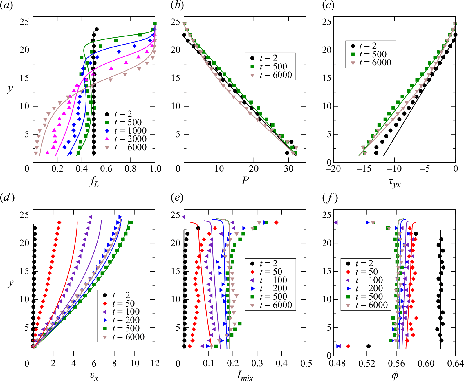
(a) Comparison of the instantaneous profiles for an equal composition binary mixture having density ratio  $\rho = 2.0$. (a) Concentration
 $f_L$, (b) pressure
 $P$, (c) shear stress
 $\tau _{yx}$, (d) mixture velocity
 $v_x$, (e) inertial number
 $I_{mix}$ and (f) solids fraction
 $\phi$. Symbols represent the DEM data and solid lines represent the continuum predictions with each colour corresponding to a different time instant. The flow starts from the initial well-mixed configuration at inclination angle
 $\theta = 25^\circ$.

We first report the results for an equal composition binary mixture with density ratio  $\rho = 2.0$. The flow is started from an initially well-mixed state at an inclination angle of
 $\theta = 25^{\circ}$. Figure 2 shows the instantaneous concentration profiles along with other flow properties of the binary mixture at different time instants. Different symbols represent the DEM data at different times, while solid lines represent the continuum model predictions. The DEM data as well as continuum predictions at a particular instant are represented by a specific colour for the ease of comparison. Figure 2(a) shows the concentration profile of light species
 $f_L$ in the mixture. Since the flow begins from an initially well-mixed state i.e.
 $f_L(y,0) = 0.5$, the continuum model predictions for the concentration profile of light species at time
 $t = 2.0$ remains almost constant (black line) with
 $f_L \approx 0.50$ for all
 $y$ values following the DEM data (black circles) closely. As time proceeds, the light particles move upwards and heavy particles move downwards leading to increase (decrease) in the
 $f_L$ values near the free surface (base) which is clearly observable from the DEM data at
 $t = 500,1000,2000$ and
 $6000$. The predicted concentration profiles also depict the same trend and follow the DEM data very well. We observe that the concentration profiles become steady after
 $t=6000$ indicating that steady-state segregation is achieved. Figures 2(b)–2(f) show the pressure, shear stress, velocity, inertial number and packing fraction profiles at different time instants. Figures 2(b) and 2(c) demonstrate that the pressure and shear stress profiles exhibit relatively small change over time due to segregation.
Figure 2(d) shows the variation of velocity in the flow direction ( $v_x$) with the distance from the base. The predicted velocity profiles for
 $50$ and
 $100$ time units are found to be reasonably higher compared with the DEM data. The deviation in the continuum model predictions at initial times can also be observed in the variation of the inertial number, shown in figure 2(e). The origin of these differences lies in the inertial number based
 $\mu {-}I$ rheological model. Figure S1 in the supplementary material shows that the fits for
 $\mu (I)$ and
 $\phi (I)$ significantly deviate form the DEM data for low inertial numbers. We also note that the validity of the inertial number based rheological description becomes questionable at very low values of the inertial numbers (Andreotti, Forterre & Pouliquen Reference Andreotti, Forterre and Pouliquen2013). After this initial time period, the predicted velocity profiles match very well with the DEM data. As expected, the instantaneous velocity at
 $t=500$ time units is found to be higher compared with that at
 $t=200$ as the flow evolves. However, the steady-state velocity at
 $t=6000$ is found to be lower than the instantaneous velocity at
 $t=500$ time units. This very interesting feature is accurately predicted by the continuum model as well. We discuss this in more detail later while discussing the results for figure 3. However, the prediction for later times agree reasonably well with DEM simulations. The variation of solids fraction (
 $\phi$) at different times is shown in figure 2(f) and the predicted profiles match well with the DEM data.
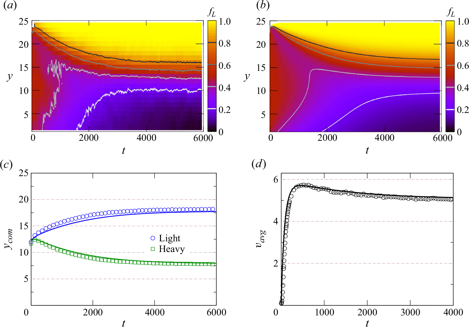
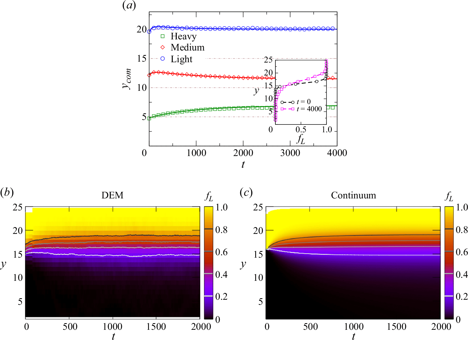
Comparison of evolution of concentration of light species ( $f_L$) with time for an equal composition binary mixture with density ratio
 $ \rho = 2.0$. (a) DEM data and (b) continuum simulation. Variation of (c) the species centre of mass and (d) average mixture velocity with time. Symbols represent the DEM data, while solid lines represent the continuum model predictions.

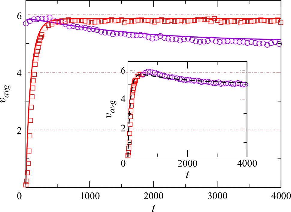
Variation of average velocity with time for monodisperse mixture. Red squares represent DEM data, while the red line represents theory data for monodisperse mixture. Purple circles/lines represent the data for the case where we increased the mass of randomly selected  $50\,\%$ particles by a factor of two, starting from the steady-state positions and velocities of the particles corresponding to monodisperse case after
 $500$ time units. Inset shows the data for the monodisperse case up to
 $500$ time units and the sudden mass change case for
 $t \geqslant 500$. Black dashed line represents model predictions for a binary mixture shown by the solid line in figure 3(d).

Variation of the light species concentration across the layer in figure 2(a) could be shown only for a few specific time instants. To get a better understanding of evolution of the concentration of light particles across both spatial as well as temporal coordinates, we plot the light species concentration using a colour map across the space–time plane in figures 3(a) and 3(b). We report the data for the case shown in figure 2, i.e. density ratio  $\rho = 2.0$ and inclination angle
 $\theta = 25^{\circ}$. Figure 3(a) shows the concentration colour map of light species obtained from the DEM simulations, while the predictions from the theory are shown in figure 3(b). In this representation, yellow denotes
 $f_L = 1$, i.e. pure light species, whereas black corresponds to
 $f_L = 0$, i.e. pure heavy species. The spatial distribution of light and heavy species across flowing layer height using the DEM data (figure 3a) matches well with the predictions (figure 3b) throughout the space–time plane. The concentration using DEM data in figure 3(a) exhibits more discrete variations compared with the continuum model, which can be attributed to the large grid size (equal to
 $d$) used in the case of DEM. The rough nature of contour lines for DEM data in figure 3(a) compared with the smooth contour lines of continuum simulations in figure 3(b) can also be attributed to the same reason. The black, dark grey, light grey and white colour contour lines correspond to
 $f_L = 0.8,0.6,0.4$ and
 $0.2$, respectively. The white region near the top represents the region beyond the free surface.
For a more quantitative comparison of the theory with DEM simulations, we report the variation of the centre of mass of the species  $y_{com}$ with time
 $t$. Figure 3(c) shows the variation of
 $y_{com}$ for both light (blue) and heavy (green) species in the mixture. Symbols represent the DEM data, while solid lines represent the continuum model predictions. Initially at time
 $t = 0$,
 $y_{com}$ is identical for both species since the flow is started from a well-mixed configuration. The centre of mass of the heavy species decreases while that of light species starts to increase until becoming constant for
 $t \geqslant 5000$ and the continuum predictions describe the DEM data very well. Figure 3(d) shows the variation of average mixture velocity along the flow direction (
 $v_{avg}$) with time. While a rapid increase in
 $v_{avg}$ is observable at early times, the flow velocity reaches a maximum around
 $500$ time units and then slowly decreases afterwards. This non-monotonic variation of the average flow velocity with time is very well captured by the continuum model as well. This demonstrates the capability of the one-dimensional continuum model which is able to capture the intricate details and subtle nuances of the flow and segregation features observed in DEM simulations. The non-monotonic variation of
 $v_{avg}$ with time occurs due to the inter-coupling of the rheology and segregation. This peculiar behaviour can be better understood by considering two different flow situations that minimise the effects of the inter-coupling between rheology and segregation. In the first case, we remove the segregation altogether and consider the average velocity variation with time for a monodisperse granular material starting from rest. We plot
 $v_{avg}$ for monodisperse material in figure 4 using red squares (DEM data) and solid red lines (model). For this case,
 $v_{avg}$ increases with time and reaches a plateau around
 $500$ time units. This rising behaviour at early times is similar to the early-time behaviour observed in figure 3(d), confirming that the early rise of
 $v_{avg}$ with time occurs due to the acceleration of the layer. To simulate a situation where the inter-coupling of segregation with rheology is minimal, we use the following protocol. Starting from the steady-state positions and velocities of the particles corresponding to the monodisperse case, we randomly selected
 $50\,\%$ particles in the layer and increased their mass by a factor of two. This protocol provides us with a well-mixed mixture with an initial velocity equal to that for the steady flow of monodisperse granular material of the same density. Using this combination of the initial species composition and velocity of the particles, we performed the DEM simulations as well as continuum simulations and observed the variation of the average flow velocity and species centre of mass. The results from these DEM simulations are shown using purple circles and the continuum model predictions are shown using solid lines of the same colour in figure 4. The
 $v_{avg}$ for this case keeps decreasing with time. The inset in figure 4 shows that figure 3(d) can be approximately reconstructed by combining the monodisperse data (red symbols) of figure 4 up to
 $500$ time units with the data for the sudden change in the particle density case for the fully developed flow (purple symbols). The black dashed line in the inset corresponds to the model predictions shown in figure 3(d). The excellent agreement of the black dashed line with the data confirms that the initial rise in the average velocity occurs primarily due to acceleration of the layer. Further, the slow decreasing behaviour of
 $v_{avg}$ in figure 3(d) occurs due to the slow evolution of segregation during the flow. Due to the dependence of the mixture viscosity on local concentration in the inertial number based rheological model, a complex interplay of the segregation and rheology during the flow occurs. Since the segregation occurs over a large time scale, the viscosity of the granular mixture also keeps changing and leads to slow decrease of the average velocity. The proposed continuum model accounts for this inter-coupled nature of rheological and segregation model, and hence, this interesting non-monotonic behaviour of average velocity is captured very accurately by the model. It is important to note that in the absence of the inter-coupling of the rheology with segregation, such flow features cannot be captured.
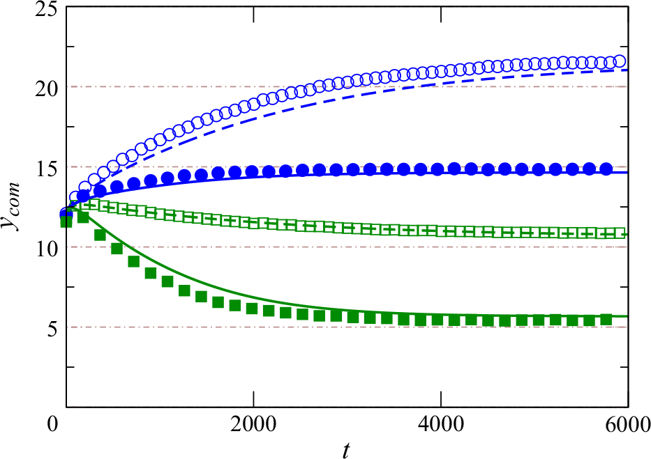
Figures 2 and 3 confirm that the particle force-based theory is successfully able to predict the time-dependent segregation for equal composition binary mixtures. We next report the results for two different mixture compositions. As before, the flow is started from an initial well-mixed state at an inclination angle  $\theta = 25^{\circ}$ and the density ratio of the heavy to light species is
 $\rho = 2.0$. Figure 5 shows the time variation of the centre of mass position of light and heavy species for two different composition mixtures. Empty symbols correspond to DEM data for a mixture having
 $20\,\%$ light particles (
 $f^T_L = 0.20$), while filled symbols correspond to DEM data for mixture having
 $80\,\%$ light particles (
 $f^T_L = 0.80$). Starting from a uniform concentration of
 $f_L = f^T_L$, the concentration of light species keeps decreasing near the base and keeps increasing near the top as time progresses. For the case of
 $f^T_L = 0.20$, the centre of mass for light species (blue colour) rises from
 $y_{com}\approx 12$ to
 $y_{com}\approx 22$, whereas for
 $f^T_L = 0.80$, it reaches only up to to
 $y_{com}\approx 15$. Figure 5 shows that the model predictions (dashed lines for
 $f^T_L = 0.20$ and solid lines for
 $f^T_L = 0.80$) are in reasonably good agreement with DEM data (symbols). Figure S2 (refer to § SM3 of the supplementary material) also shows that the instantaneous concentration profiles and colour maps of light species using the continuum model agree well with the DEM data.
Time evolution of centre of mass ( $y_{com}$) for two different composition mixture for density ratio
 $\rho = 2.0$ at inclination angle
 $\theta = 25^\circ$. Empty symbols along with the dashed lines represent the data for a mixture with
 $20\,\%$ light species (
 $f^T_L = 0.2$), while filled symbols along with the solid lines correspond to the
 $f^T_L = 0.8$ case.

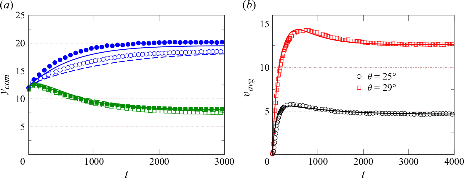
Time variation of (a) centre of mass ( $y_{com}$) and (b) average velocity (
 $v_{avg}$) for an equal composition binary mixture with density ratio
 $\rho = 3.0$ flowing at
 $\theta = 25^\circ$ and
 $\theta = 29^\circ$.

Next, we explore whether the proposed theory is able to capture the influence of the inclination angle on the mixture flow and segregation. Figure 6 shows the results for an equal composition binary mixture with density ratio  $\rho = 3.0$. As before, the data are reported for a mixture starting from well-mixed initial configuration. Figure 6(a) shows time variation of the species centre of mass for both heavy (green) and light (blue) species flowing at inclination angles
 $\theta = 25^{\circ}$ and
 $\theta = 29^{\circ}$. Here, the empty symbols along with the dashed lines represent the DEM data and model predictions for inclination angle
 $\theta = 25^{\circ}$. The filled symbols and solid lines correspond to the DEM data and the prediction of the model for
 $\theta = 29^{\circ}$. The corresponding average mixture velocity is shown in figure 6(b). As before, the average velocity for both inclinations rises quickly, achieves a maximum value and then starts to slowly decrease due to the inter-coupling of rheology and segregation. The steady-state average mixture velocity at inclination angle
 $\theta = 29^{\circ}$ (red) is more than twice of the steady-state average velocity at
 $\theta = 25^{\circ}$ (black). Continuum model predictions (shown using lines) are in very good agreement with DEM simulation data (symbols) for both these inclination angles. We have also performed simulations for different binary mixtures with density ratios
 $\rho = 1.5, 2.0, 3.0$ and
 $5.0$ over a wide range of compositions and inclination angles. While these results are not reported here to avoid repetition, we find that the continuum model predictions for all these different cases are found to be in very good agreement with DEM simulations. Hence, we conclude that the particle force-based theory for a binary mixture is successfully able to predict the evolution of segregation over a wide range of concentrations, inclination angles and density ratios. In addition, we find that the continuum model is able to account for the dependence of the DEM simulation parameters (§ SM4 of the supplementary material). The relative importance of various continuum model parameters has also been investigated and is reported in § SM5 of the supplementary material.
4.2. Comparison with kinetic theory (Larcher Jenkins 2015)
Time evolution of centre of mass ( $y_{com}$) for an equal composition binary mixture having density ratio
 $\rho = 2.0$ at inclination angle
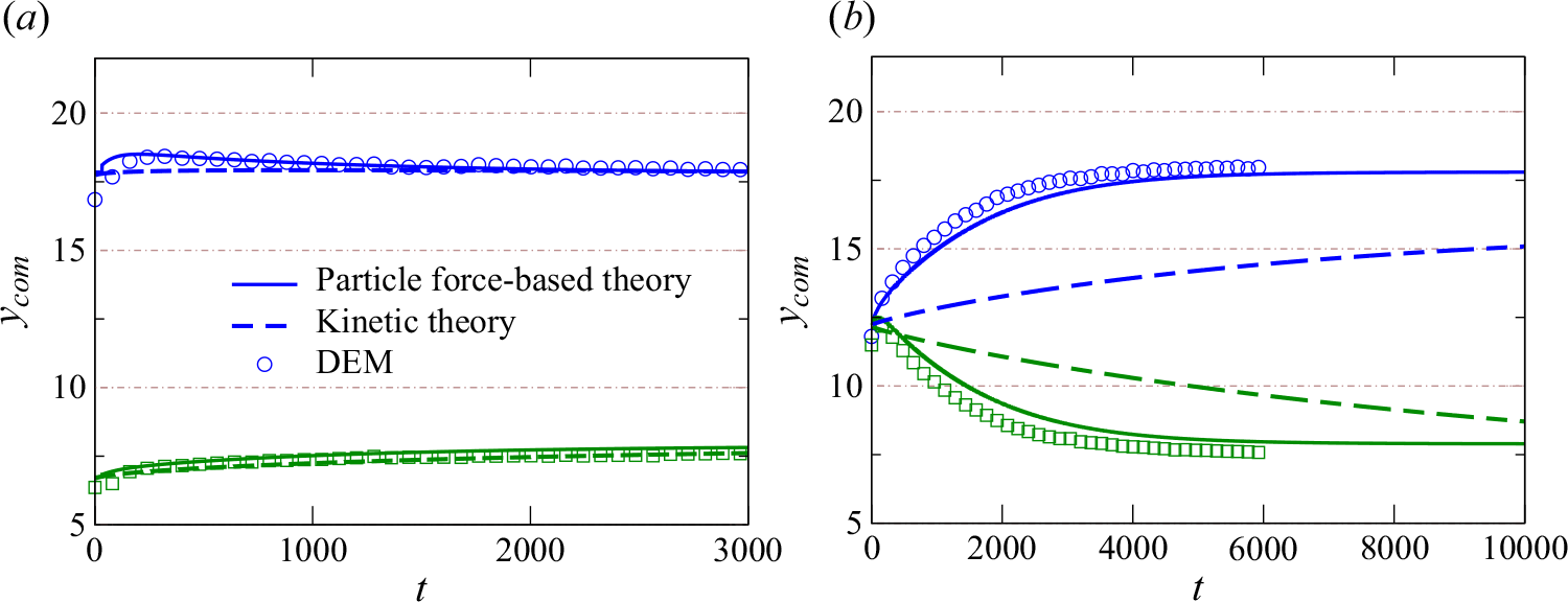
 $\theta = 25^\circ$ for two different initial configurations: (a) heavy-near-base and (b) well-mixed configuration. Symbols represent the DEM data, solid lines represent the predictions using the particle force-based segregation model, while dashed lines represent predictions using the kinetic theory model of Larcher & Jenkins (Reference Larcher and Jenkins2015). The blue colour corresponds to the light species and the green colour corresponds to the heavy species.

Larcher & Jenkins (Reference Larcher and Jenkins2015) have proposed a kinetic theory-based model to predict the evolution of segregation of binary granular mixtures in the dense flow regime for small size and density differences. In this section, we use their kinetic theory-based model to predict density segregation in a periodic chute and compare the predictions of their model with the present work. We solve the partial differential equation given by Larcher & Jenkins (Reference Larcher and Jenkins2015) (( $3.10$) of their work) along with the boundary conditions ((
 $4.3$) of their work) using the MATLAB PDEPE solver. For these predictions, we have used the same model parameters as used by these authors. For a meaningful comparison, the flowing layer thickness has been chosen equal to that used in the present work. Using their model, we predict the evolution of segregation for two different initial configurations of the mixture, namely heavy-near-base configuration and well-mixed configuration. Figure 7 shows the results for an equal composition binary mixture having density ratio
 $\rho = 2.0$ flowing at inclination angle
 $\theta = 25^\circ$. Figure 7(a) shows the time variation of the centre of mass of both heavy (green) and light (blue) species starting from the heavy-near-base configuration. Solid lines represent the predictions using the particle force-based model, while dashed lines represent predictions using the kinetic theory model of Larcher & Jenkins (Reference Larcher and Jenkins2015). Both models capture the evolution of segregation very well for this initial segregated state. Figure 7(b) shows the time variation of the centre of mass of both heavy (green) and light (blue) species starting from the well-mixed configuration. Predictions using kinetic theory (dashed lines) significantly deviate from the DEM data for both the species. Specifically, the time scale for segregation using the kinetic theory model for this initial state is much larger compared with that observed in the DEM simulation. While the DEM simulation shows that the centre of mass of the species becomes nearly constant after approximately 4000 time units, kinetic theory predictions for the species centre of mass do not reach a constant value even after 10 000 time units. Similar discrepancies are reported by the authors in the case of size segregation (figure 1 of Larcher & Jenkins Reference Larcher and Jenkins2015) for the well-mixed configuration of different size mixtures. The authors do acknowledge this limitation of their model prediction and report that the rate of evolution of segregation according to their theory is slower as compared with DEM simulations and experimental data available in the literature. While the authors suggest that adjustment of the kinetic theory model parameters may be helpful in predicting this rate of evolution in better agreement by DEM simulations, we were unable to observe good agreement of the time evolution and the steady-state values of the centre of mass of the species with the DEM simulations despite varying the parameters in the kinetic theory over a wide range.
5. Segregation evolution of multicomponent mixtures
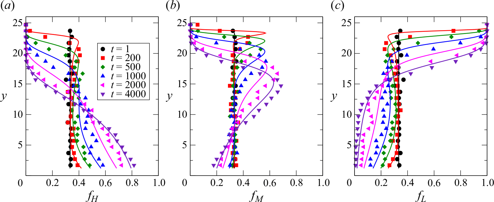
Instantaneous concentration profiles of (a) high-density, (b) medium-density and (c) low-density species in an equal composition ternary density mixture having density ratios  $\rho _H: \rho _M : \rho _L$ =
 $3:2:1$. Flow is started from an initial mixed configuration at inclination angle
 $\theta = 25^\circ$.

In this section, we report the results for mixtures having more than two species. Figure 8 shows the results for a ternary mixture having equal composition of each of the three species  $f^T_L = f^T_M = f^T_H = 1/3$. Species density ratios are
 $\rho _H: \rho _M : \rho _L$ =
 $3:2:1$ and the flow starts from a well-mixed initial configuration at inclination angle
 $\theta = 25^{\circ}$. Figure 8(a) shows the instantaneous concentration profiles of the heavy species at different time instants. The concentration profiles for medium and light species are shown in figures 8(b) and 8(c), respectively. Symbols represent the DEM data, while solid lines represent continuum model predictions. Different colours correspond to model predictions at different times. Initially, at time unit
 $t = 2$, the concentrations of heavy, medium and light species are
 $1/3$ throughout the layer height as the flow starts from a uniformly mixed state. As the flow evolves, the concentration of heavy species increases near the base and decreases near the free surface due to segregation. At
 $t = 4000$, the concentration of heavy species (purple line and symbols) is found to be zero near the free surface (see figure 8a). Similarly, the light particles experience net upward force in the presence of medium- and high-density particles. Hence, the concentration of light species decreases gradually towards the base with time, as shown in figure 8(c). The medium-density particles, however, experience an upward force in the basal region rich in high-density particles and a downward force in the free surface region rich in low-density particles. Hence, the concentration of medium-density species decreases near the base as well as near the surface with time. Increasingly more medium-density particles concentrate in the middle part of the layer with time and, hence, the concentration of medium species at
 $t = 4000$ is larger in the middle region compared with the free surface and base, as shown in figure 8(b).
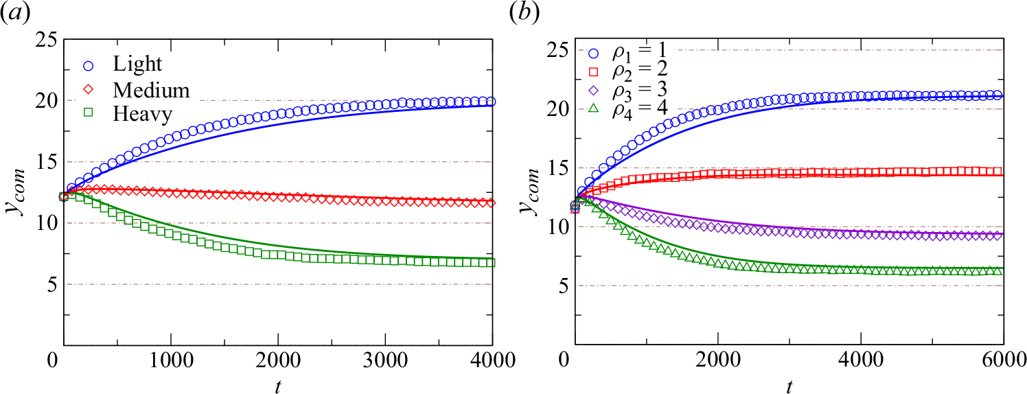
Time evolution of the centre of mass of all species in equal composition mixtures flowing at inclination angle  $\theta = 25^\circ$. (a) Ternary mixture having density ratios
 $\rho _H: \rho _M : \rho _L$ =
 $3:2:1$ and (b) quaternary mixture having density ratios
 $\rho _4: \rho _3 : \rho _2 : \rho _1 = 4:3:2:1$.

Figure 9(a) shows the variation of the centre of mass  $y_{com}$ with time for this equal composition ternary mixture. Evidently, predictions (solid lines) using the continuum model match well with the DEM data (symbols) for all the three species for the case of a ternary mixture as well. Figure 9(b) shows the variation of the centre of mass of the species for a quaternary mixture having density ratios
 $\rho _4: \rho _3 : \rho _2 : \rho _1 = 4:3:2:1$ starting from a well-mixed initial configuration at inclination angle
 $\theta = 25^\circ$. Again, an excellent match is observed between the DEM simulations and continuum model predictions for this case as well, without using any fitting parameter in the theoretical formulation. These results confirm that the proposed continuum model is able to capture the time evolution of the flow and segregation for multicomponent mixtures as well.
6. Effect of initial configuration of species
All the results reported above considered mixtures having a well-mixed initial configuration. We now report results exploring the applicability of our one-dimensional segregation model to capture the flow evolution for different initial configurations for binary and ternary density mixtures. Specifically, we consider the cases for binary and ternary mixtures with an initial configuration that is nearly completely segregated.
6.1. Heavy-near-base configuration
(a) Time variation of species centre of mass ( $y_{com}$) starting from the initial concentration profile (
 $t = 0$) shown in the inset. Variation of concentration of light species across the layer height with time for a ternary mixture with
 $\rho _H: \rho _M: \rho _L = 3:2:1$ starting from the heavy-near-base initial configuration at an inclination angle
 $\theta = 25^\circ$ from (b) DEM simulations and (c) continuum model predictions.

We first consider mixtures with high-density species located near bottom of the layer. The results for the binary mixture case are shown in figure S6 of the supplementary material and we present the results only for the ternary mixture case here. Figures 10(a)–10(c) show the results for an equal composition ternary mixture having density ratios  $\rho _H: \rho _M: \rho _L = 3:2:1$ and flowing at
 $\theta = 25^\circ$. The flow starts from a heavy-near-base configuration in which high-density particles are kept near the bottom and light-density particles are kept near the surface with the medium-density particles sandwiched in between the two. Time variation of
 $y_{com}$ for all the three species are shown in figure 10(a). Symbols represent the DEM data and solid lines represent continuum predictions. A very good match between the two is observed. Figures 10(b) and 10(c) show concentration colour maps of the light species obtained from the DEM and continuum simulations, respectively. Since the initial concentration of light species is present only near the upper one third of the layer in this case, the yellow region with
 $f_L = 1$ is observed near the top portion of the layer at early times along with narrow regions of red and purple (corresponding to the linear part of the concentration data shown in the inset of figure 10a). As time increases, the span of the yellow region across the layer appears to decrease, while that of the red and purple regions increase due to the diffusional mixing. This diffusional mixing observed in the concentration colour maps obtained from the DEM simulation is very well captured by the continuum model as well. The white, light grey, dark grey and black colour contour lines correspond to
 $f_L =0.2, 0.4, 0.6$ and
 $0.8$, respectively. Again, the agreement between DEM simulations and continuum predictions in figures 10(b) and 10(c) is found to be pretty good. Similar results are observed for heavy
 $f_H$ and medium species
 $f_M$ (not shown here) as well.
(a) DEM snapshot for an equal composition binary mixture of density ratio ( $\rho = 2.0$) for the light-near-base configuration. Green spheres represent the high-density particles, while blue spheres represent the low-density particles. The orange arrow indicates the direction of flow. (b) Time evolution of
 $y_{com}$ for both light (blue) and heavy (green) species using DEM data (symbol) and model predictions (solid lines). Colour map of light species concentration in the flowing layer over time range using (c) DEM and (d) continuum model at inclination angle
 $\theta = 25^{\circ}$.

6.2. Light-near-base configuration
We next report the results for the cases where the heavy species is near the free surface and the light species is near the base at the starting of the simulation. Figure 11(a) shows the DEM snapshot of the initial configuration for an equal composition binary mixture having density ratio  $\rho = 2.0$. The flow occurs at
 $\theta = 25^\circ$ and the variation of
 $y_{com}$ of both light and heavy species with time is shown in figure 11(b). The centre of masses of both the species rise for a brief initial period (up to
 $250$ time units) due to the layer dilation. After that, a sharp rise in the
 $y_{com}$ of light species (blue circles) and sharp decline in the
 $y_{com}$ of heavy species (green squares) is observed from the DEM simulations (symbols) during the next
 $250$ time units. After
 $t = 500$ time units,
 $y_{com}$ of both the species change gradually. In contrast to all other cases considered before, the predicted centre of mass from the continuum model (shown using solid lines) deviates significantly from the DEM data. It is evident that the model fails to capture the centre of mass behaviour observed in the case of DEM simulations.
The concentration colour map of the light species, as obtained from the DEM simulations, is shown in figure 11(c). The predictions from the continuum model are shown in figure 11(d). Lines in the colourmaps correspond to contour lines of different  $f_L$ values as before. Evidently, the predicted behaviour from the model is qualitatively different from that observed in the DEM simulations. The concentration colour map from the DEM simulations (figure 11c) show that the yellow region (having pure light species) in the lower part of the layer disappears around
 $500$ time units and very quickly appears near the top part of the layer. In addition, the concentration of heavy species in the lower part of the layer remains high (purple region) for all times larger than
 $750$ time units except for a very brief duration, (shown by the red coloured region in the lower part of the layer), where both the species appear to be well-mixed. The continuum model predictions in figure 11(d), however, show a gradual decrease in the light species concentration in the lower part of the layer and high concentration of heavy species (purple region) is observable only after
 $3000$ time units. Similarly significant qualitative differences are observable in the upper part of the layer as well where the contour line for a given colour corresponding to a particular
 $f_L$ shows very different trend in DEM simulation as compared with the continuum prediction.
We further investigate this configuration for a ternary mixture, in which particles with low density are concentrated near the base, medium-density particles are positioned in the middle and particles with high density are located at the top. Figure 12(a) shows the DEM snapshot of such an initial configuration where green, red and blue spheres represent the high-, medium- and low-density particles, respectively, and black spheres represent the static particles that form the rough, bumpy base. Figure 12(b) shows the variation of  $y_{com}$ for all three species in the mixture. As before, symbols represent the DEM data and lines correspond to predictions obtained from continuum model. As in the case of a binary mixture, DEM data show a very quick change in the centre of mass of the heavy (green) and light (blue) species, while the theoretical lines show a gradual variation. Evidently, the quick segregation observed in the initial
 $500$ time units is not captured by the model. Visible qualitative differences are observable in the concentration colour maps of the light species obtained from the DEM simulations (figure 12c) and the continuum model (figure 12d). Figures 12(e) and 12(f) show the concentration colour map for the heavy species and notable qualitative differences are observable between the model and the DEM simulations. The contour lines for the DEM and continuum predictions show very different trends for this initial configuration in the case of a ternary mixture as well. Similar differences are also observed in the concentration colour maps of medium-density species as well (not shown here).
DEM snapshot of a ternary mixture having density ratio  $\rho _H: \rho _M: \rho _L = 3:2:1$ for the light-near-base initial configuration at inclination angle
 $\theta = 25^\circ$. Green, red and blue particles represent the high-, medium- and low-density particles, respectively. Black particles represent the rough bumpy base of thickness
 $1.2d$. The orange arrow indicates the direction of flow. (b) Variation of
 $y_{com}$ with time for all species. Colour map for the concentration of light species using (c) DEM and (d) continuum model. (e) and (f) The same for the heavy species.

7. Rayleigh–Taylor-like instability in granular mixture flows
The results shown in figures 11 and 12 confirm that the model is unable to capture the evolution of segregation for the cases when the heavy species is situated at the top of the layer. The sudden changes in the species centre of mass as well as the light and heavy species concentration colour maps observed in the DEM simulations indicate that the mechanism of segregation operative in this case is not captured using our one-dimensional continuum model. To identify the reason for the quick segregation observed in these cases, we take a more careful look at our DEM simulation results.
(a) Variation of  $y_{com}$ with time for a ternary mixture at early times in the case of a light-near-base initial configuration. DEM snapshots for equal composition ternary mixture at different times: (b)
 $t = 150$; (c)
 $t = 200$; (d)
 $t = 250$; (e)
 $t = 300$ and (f)
 $t = 500$ starting from the light-near-base initial configuration at inclination angle
 $\theta = 25^{\circ}$ with density ratios
 $\rho _H : \rho _M : \rho _L = 3:2:1$. The orange arrow in panel (b) indicates the direction of flow.


Figure 13(a) (in the centre) shows the variation of the centre of mass of the heavy, medium and light species for the first  $500$ time units after the flow. Figures 13(b), 13(c), 13(d), 13(e) and 13(f ) show the DEM simulation snapshots corresponding to
 $150$,
 $200$,
 $250$,
 $300$ and
 $500$ time units, respectively. The arrangement of particles at
 $t = 150$ (figure 13b) shows that the heavy (green), medium (red) and light (blue) particles occupy the upper, middle and lower part of the layer. The onset of the instability and plume formation is clearly observable in the snapshots shown in figure 13(c)–13(e). Figure 13(b) shows the existence of a small perturbation of the light–medium as well as medium–heavy interface at
 $t=150$, which grows significantly by time
 $t=200$ (figure 13c) indicating the onset of formation of a medium and light species plume. This can be more clearly observed in the snapshots shown in figure 14, where particles of only one species are shown. Figures 14(a), 14(b) and 14(c) show the arrangement of particles of heavy, medium and light species at
 $t=200$. Figure 14(a) clearly shows the significantly perturbed interface of the heavy particles. The light particles also occupy a larger height in the centre of the simulation box compared with the sides at
 $t=200$ (figure 14c), while the medium species particles appear to be in the form of a mushroom-cap (figure 14b).
Returning back to figure 13(d), we see that by the time  $t=250$, a plume of light (blue) and medium (red) species rises to the free surface due to the settling of the heavy particles from the sides. The arrangement of the particles of individual species for this particular instant is shown in figures 14(d), 14(e) and 14(f). A comparison of the heavy-species particles shown in figure 14(a) and 14(d) confirms that the interface between the heavy and medium species deforms to a large extent and almost all the heavy particles concentrate in the form of two columns at the z-boundaries of the simulation box. This settling of the heavy species from the sides pushes the medium- and low-density particles concentrated in the centre portion of the box upwards. The formation of the plume of light- and medium-species particles is clear by the column-like structural arrangement of the light species (figure 14f), which are surrounded by the medium-density particles (figure 14e). The rising plume of the light and medium species first brings the medium-density particles at
 $t=250$ (see figure 13d) and then low-density particles to the top at
 $t=300$ (figure 13e). The medium-density particles quickly settle downwards leaving a pure layer of the light species at the top which grows further in thickness as time progresses to
 $t=500$ (figure 13f).
Thus, the instability quickly drives the light-near-base and heavy-at-the-top arrangement of particles into a configuration where the heavy species concentrates near the base and the light species gets concentrated near the free surface with the medium species occupying the space between these two species. This situation is reminiscent of the Rayleigh–Taylor instability observed in the case of classical fluids when a high-density fluid displaces a low-density fluid. We note that this instability is observable in the  $yz$ plane and forms a plume pattern of the light and medium species in the
 $y$ direction. Similar instabilities have been observed by D’Ortona & Thomas (Reference D’Ortona and Thomas2020) in the case of binary mixtures having particles of different densities and sizes flowing over a periodic chute. The results for the binary mixture case, shown in figure S7 of the supplementary material, also depict the presence of instability for the case of heavy species on top of light species.
The arrangement of particles depicted in figure 13(f) is very similar to the configuration studied in figure 10. Given the successful prediction of the centre of mass for the configuration in figure 10(a) from our model, we expect that the model should be able to capture the evolution of the species concentrations and species centre of masses reasonably well from this time onwards. Hence, we use the DEM data at  $t = 500$ to obtain the concentration profile
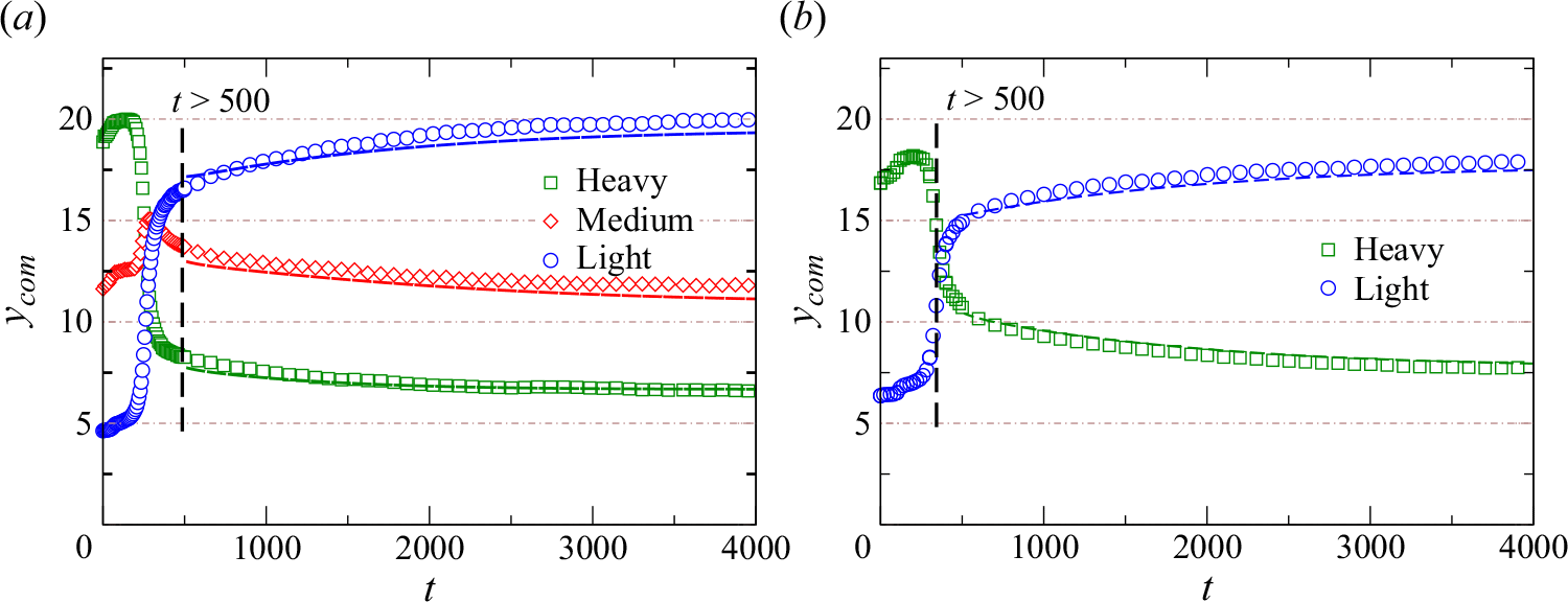
 $f_i(y)$ of the three species at this particular instant (snapshot shown in figure 13f) as the initial condition in the continuum model and predict the evolution of the species centre of mass for the ternary mixture. These model predictions are shown as dashed lines in figure 15(a), while symbols represent the DEM data. Interestingly, the theory can accurately predict the segregation behaviour for
 $t \gt 500$ time units by using the concentration profiles at
 $t=500$ as the initial condition. The concentration colour maps from the continuum model predictions are also found to be qualitatively as well as quantitatively very similar to those obtained from the DEM simulations for
 $t\gt 500$ (shown in figure 12c and 12e) and hence are not shown for the sake of brevity. Similarly, figure 15(b) shows the centre of mass evolution for the binary mixture case with heavy species on top (see figure 11a) using the concentration profiles of heavy and light species at
 $t=500$ for the snapshot shown in figure S7(f) of the supplementary material. Again, the continuum model predictions for the centre of mass are in very good agreement with the DEM data for
 $t\gt 500$.
Time evolution of  $y_{com}$ for the light-near-base configuration after
 $t = 500$ time units when the quick segregation due to instability is over. (a) Equal composition ternary mixture having density ratios
 $\rho _H : \rho _M : \rho _L = 3:2:1$ and (b) equal composition binary mixture having density ratio
 $\rho = 2.0$ for inclination angle
 $\theta = 25^{\circ}$.

The results shown in figures 15(a) and 15(b) confirm that the continuum model fails to predict the centre of mass evolution only for the brief time interval during which the instability occurs for the higher density species on top of lower density species configurations. This is not unexpected since the continuum model accounts for property variations only along the  $y$ direction and ignores the variations along the other two directions. While this assumption is reasonable for the well-mixed and heavy-near-base configurations studied in this work, it is not valid for the duration over which the instability is observed for the configurations with high-density species at the top. The snapshots shown in figure 13 confirm that the velocity as well as the species concentrations vary in all three directions. Hence, the momentum balance equations along with the rheological and segregation model must be solved in the three dimensions to be able to capture the flow and segregation due to the onset of the instability and the resulting quick segregation for heavy-on-top configurations. The snapshots depicting the position of the particles of the individual species (shown in figure 14) suggest that a two-dimensional model accounting for the variations in
 $y$ and
 $z$ direction may also be sufficient to capture the essential features since the variations along the flow direction do not seem to be very significant. Recently, D’Ortona et al. (Reference D’Ortona, Lueptow and Thomas2024) have suggested the existence of Rayleigh–Taylor instability in rotating tumblers for different size mixtures using their DEM simulation data, where the radial segregation leads to a small region of increased density due to more efficient packing of large and small grains, which ultimately leads to axial segregation of size-bidisperse granular mixtures. More detailed investigations about different aspects of the granular Rayleigh–Taylor instability are needed to gain a better understanding of these observations, including the spanwise wavelength of the longitudinal rolls.
8. Summary
In this work, we have developed a continuum model to predict the time-dependent density segregation for binary as well as multicomponent mixtures in a periodic chute flow. The model incorporates a transient segregation–diffusion equation for all the species along with an inertial number based mixture rheological description to solve the momentum balance equations for same-size, different-density granular mixtures. Specifically, the segregation model uses the particle force-based theory proposed by Sahu et al. (Reference Sahu, Kumawat, Agrawal and Tripathi2023) to calculate the segregation velocity. In contrast to the existing empirical segregation models (Xiao et al. Reference Xiao, Umbanhowar, Ottino and Lueptow2016; Jones et al. Reference Jones, Isner, Xiao, Ottino, Umbanhowar and Lueptow2018) for density segregation, the particle force-based model does not require any empirical parameter. The generalised form of the inertial number based rheology (Jop et al. Reference Jop, Forterre and Pouliquen2006) for granular mixtures, proposed by Tripathi & Khakhar (Reference Tripathi and Khakhar2011), is used to capture the flow evolution. It is important to note that solving the segregation–diffusion equation requires knowledge of the flow kinematics. Unlike most other approaches that use the flow kinematics data obtained from experiments or DEM simulations, we solve the time-dependent momentum balance equations by inter-coupling the mixture rheology and the segregation model. Due to the inter-coupling of rheology and segregation, the predictions from our model are able to capture non-monotonic evolution of the velocity field in the case of well-mixed initial configuration. Continuum model predictions use the no-slip boundary condition at the base, which is simulated by using a rough and bumpy base in DEM. For granular flows involving flat surfaces, however, the presence of a finite slip velocity at the base might need to be accounted for. The model is able to predict the concentration profiles and flow properties such as velocity, shear stress, pressure, solids fraction and inertial number reasonably well for two different initial configurations. In addition, the model successfully captures the segregation for different mixture compositions, density ratios and inclination angles. Significant differences, however, are observed in the predicted velocity profiles as compared with DEM data for a small time period after the start of the flow. These discrepancies are attributed to the limitations of the rheological model to describe flow at low inertial numbers. We have also investigated the effect of microscopic, particle-level properties on the evolution of macroscopic properties of the flow such as average mixture velocity and species centre of mass. As expected, the inter-particle friction coefficient affects the average mixture velocity significantly due to its strong influence on the rheological parameters. The proposed continuum model is able to account for this effect by incorporating appropriate rheological parameters corresponding to the microscopic particle properties. While the segregation does not get significantly altered by ignoring the anisotropy of the normal stresses, the average velocity of the mixture gets under-predicted by ignoring the normal stress differences. Further, the dilatancy effects can also be ignored by using a constant solids fraction in the dense flow regime. In addition to the proposed continuum model, kinetic theory-based predictions of segregation evolution have also been compared with DEM simulations. These predictions demonstrate good quantitative agreement only for the heavy-near-base configuration and exhibit significantly slower evolution of the segregation in the case of a well-mixed initial configuration.
While the properties of the well-mixed initial configuration as well as heavy-near-base initial configurations are predicted very well using our continuum model, the model does not accurately capture the behaviour for the light-near-base initial configuration. For this configuration, quick segregation is observed at early times followed by a slow evolution of the segregation at later times. The model fails to capture the quick segregation despite the inter-coupling of rheology and segregation due to its one-dimensional nature. By carefully observing DEM snapshots at different time instants during this quick segregation phase, we notice the presence of a Rayleigh–Taylor-like instability due to the unstable initial configuration of high-density species being on top of a low-density species. The slight perturbations of the species interface at early times are followed by bulk motion where the heavy species quickly moves downwards and pushes the lighter species upwards. Once the bulk motion induced due to the onset of instability subsides, the light species concentrates near the top and the heavy species gets concentrated near the base. By using the species concentration profiles at the end of this quick segregation phase as the initial concentration profile, the model is able to capture the evolution of all the flow properties at later times very well. Thus, the one-dimensional formulation presented in this work fails to capture the segregation and evolution of the flow properties only for the small time duration when bulk motion and segregation in more than one dimension become important. Tirapelle et al. (Reference Tirapelle, Santomaso, Richard and Artoni2021) also used the light-near-base initial configuration to study the density segregation in annular shear cell and found noticeable differences in their 1-D continuum model predictions and experiments. While the authors do not discuss the role of instability, our results indicate that the discrepancies observed could be attributed to instability driven bulk motion during the flow. These observations indicate the need to generalise our one-dimensional continuum model to three dimensions. The continuum approach presented in this work can be easily extended to different size mixtures by incorporating the particle force-based segregation theory of Tripathi et al. (Reference Tripathi, Kumar, Nema and Khakhar2021) to predict transient size segregation in periodic chute flows. In addition, it would be interesting to explore whether a quantitative comparison with DEM simulations can be observed using this approach for long chutes and in other free surface flows such as plane shear flow or heap flow.
Supplementary material.
Supplementary material is available at https://doi.org/10.1017/jfm.2025.207.
Acknowledgements.
S.K. acknowledges the help of Mr Satyabrata Patro in performing the DEM and continuum simulations. The authors also acknowledge discussions with Professor V. Shankar (IIT Kanpur) regarding the Rayleigh–Taylor-like instability.
Funding.
A.T. gratefully acknowledges the financial support provided by the Indian Institute of Technology Kanpur via the initiation grant IITK/CHE/20130338. A.T. and S.K. gratefully acknowledge the funding support provided to S.K. by the Prime Minister’s Research Fellowship (Government of India) grant.
Declaration of interests.
The authors report no conflict of interest.
Data availability statement.
The data that support the findings of this study are available from the corresponding author, A.T., upon reasonable request.