1 Introduction
The meridional overturning component of the ocean circulation can be regarded as a conveyor belt, transporting heat, salt and other tracers such as CO
 $_{2}$
in the ocean. It carries approximately half of the total heat accumulated in the equatorial regions towards high latitudes (Vonder Haar & Oort Reference Vonder Haar and Oort1973; Wunsch Reference Wunsch2005), greatly reducing the equator to pole surface temperature contrast induced by the latitudinal variation of solar radiation. Despite increasing awareness of this circulation’s significance in regulating the Earth’s climate, progress in understanding the subject has been relatively slow, and several major issues persist. Among them, the forcing of the circulation is fundamental, and much of the consideration as well as debate has been over the relative importance of the differential buoyancy forcing at the ocean surface and the diapycnal mixing in the ocean interior.
Based on a series of laboratory experiments on circulation driven solely by thermal forcing, Sandström (Reference Sandström1908, Reference Sandström1916) speculated that a closed steady circulation could only be maintained if the stabilizing buoyancy source is located at a lower level than the destabilizing buoyancy source. According to this hypothesis, often referred to as Sandström’s theorem, the differential buoyancy forcing for the ocean, which is mostly located at the sea surface, cannot drive a large-scale circulation without extra mechanical energy supporting interior mixing. Although as early as 1925, Jeffreys (Reference Jeffreys1925) pointed out that Sandström’s theorem was flawed because it ignored the effects of molecular diffusion, it was not until the 1960s that horizontal convection (HC hereinafter), a flow resulting from a buoyancy variation imposed along a horizontal boundary (Stern Reference Stern1975), was successfully demonstrated for the first time by Rossby (Reference Rossby1965) with laboratory experiments. He reported a single persistent convecting cell of marked asymmetric structure in a non-rotating, rectangular tank with differential heating imposed along the bottom. Though qualitatively similar features were found between HC and the overall picture of the oceanic overturning circulation (Miller Reference Miller1968; Beardsley & Festa Reference Beardsley and Festa1972; Rossby Reference Rossby1998; Coman, Griffiths & Hughes Reference Coman, Griffiths and Hughes2006; Hughes & Griffiths Reference Hughes and Griffiths2008), their remarkable differences compelled investigations on additional processes that could enable a better match with the ocean. For example, as demonstrated by several studies, extra mechanical stirring or mixing can substantially affect the structure and strength of the flow (Whitehead & Wang Reference Whitehead and Wang2008; Tailleux & Rouleau Reference Tailleux and Rouleau2010; Ilicak & Vallis Reference Ilicak and Vallis2012; Stewart Reference Stewart2012). This is consistent with the well-accepted hypothesis that the diapycnal diffusion induced by turbulent processes such as breaking of internal waves is vital for both the overturning circulation and the related heat transport (Munk & Wunsch Reference Munk and Wunsch1998).
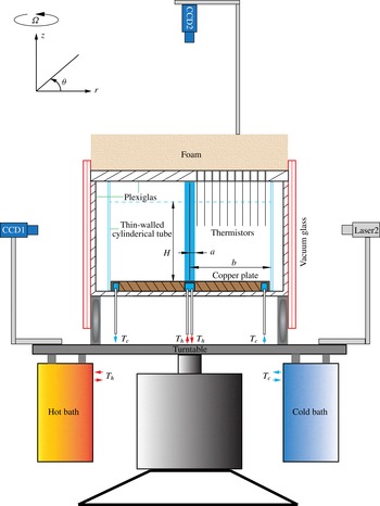
A schematic view of the experimental apparatus. The working fluid was contained in the open region bounded by two thin-walled cylindrical tubes. The fluid was heated and cooled at its lower boundary by two baths as described in the text.

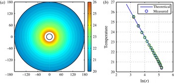
(a) Typical distribution of base temperature in the equilibrium state. (b) Radial profile of temperatures measured on the copper base (circles). They are measured at
 $16$
different radial locations and along different radial directions with increments of
 $10^{\circ }$
polar angle. The solid line denotes the theoretical value
 $T\sim \ln (r)$
.

What we are concerned with in the current study is the basic HC model and the essential ‘facts’ it can disclose for the oceanic overturning circulation. Since rotation is one of the two most fundamental features of the geophysical fluids, its effect on HC must be thoroughly understood before proceeding on to other issues. HC with rotation is not a new topic. Scaling laws for the thermal boundary layer and the lateral heat flux have been explored (Stern Reference Stern1975). Dynamics, as being controlled by the parameter
 $Q$
defined as the square of the ratio of the non-rotating thermal layer thickness to the viscous Ekman layer thickness, has been discussed (Hignett, Ibbetson & Killworth Reference Hignett, Ibbetson and Killworth1981; Park & Whitehead Reference Park and Whitehead1999; Barkan, Winters & Smith Reference Barkan, Winters and Smith2013; Sheard, Hussam & Tsai Reference Sheard, Hussam and Tsai2016). More recently, direct numerical simulations were used to examine effects of rotation on aspects such as energetic, heat transfer and baroclinic eddies within a relatively wide range of
 $Q$
(Barkan et al.
Reference Barkan, Winters and Smith2013; Hussam, Tsai & Sheard Reference Hussam, Tsai and Sheard2014; Sheard et al.
Reference Sheard, Hussam and Tsai2016). Unlike these aforementioned studies, we focus on the physics governing essential differences between rotating and non-rotating HC. We will demonstrate, using laboratory experiments performed in an annular gap with and without rotation or a full radial barrier, that potential vorticity (PV hereinafter) can impose a strong constraint on the meridional flow, affecting both the pattern and strength of the overall overturning. Thus PV is another decisive ingredient besides buoyancy forcing and diapycnal mixing for the overturning circulation, but has not been given enough attention in recent decades. Details of the experimental apparatus and measurements are described in § 2. We then present results in § 3, and finally give a summary and discussion in § 4.
2 Experiments
2.1 Apparatus
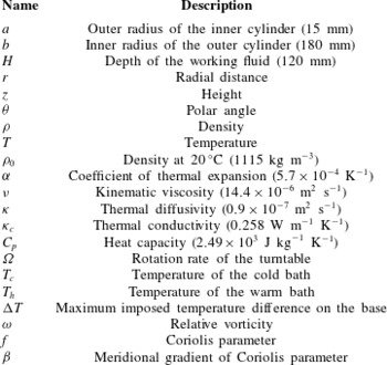
We applied the differential buoyancy forcing at the bottom of the annular gap by maintaining a radially varying distribution of temperature. As shown in figure 1, the annular gap, bounded by two coaxial Plexiglas cylinders with heights of 154 mm, was filled with ethylene glycol to a depth of
 $H=120$
mm (table 1). At
 $20\,^{\circ }$
C, it has density
 $\unicode[STIX]{x1D70C}_{0}=1115~\text{kg}~\text{m}^{-3}$
, thermal expansion coefficient
 $\unicode[STIX]{x1D6FC}=5.7\times 10^{-4}~\text{K}^{-1}$
, kinematic viscosity
 $\unicode[STIX]{x1D708}=14.4\times 10^{-6}~\text{m}^{2}~\text{s}^{-1}$
, thermal diffusivity
 $\unicode[STIX]{x1D705}=0.9\times 10^{-7}~\text{m}^{2}~\text{s}^{-1}$
, thermal conductivity
 $\unicode[STIX]{x1D705}_{c}=0.258~\text{W}~\text{m}^{-1}~\text{K}^{-1}$
and heat capacity
 $C_{p}=2.49\times 10^{3}~\text{J}~\text{kg}^{-1}~\text{K}^{-1}$
. The inner cylinder is a clear one with an outer radius of
 $a=15$
mm. The outer cylinder has inner radius
 $b=180$
mm and thickness
 $2$
mm. Both cylinders were secured to a
 $d=10$
mm thick copper plate which was heated at the centre and cooled near its outer circumference by recirculating water through two circular channels that were cut inward of the copper plate from below. Water circulating in the central channel was pumped out of a hot circulator bath with the target temperature
 $T_{h}$
; while that in the outer channel was from a cold bath with temperature
 $T_{c}$
. The two circulators used were Thermo Scientific EZ COOL 80, powerful enough to maintain temperature to the target value with an accuracy of
 $\pm 0.1$
K. Thermal conduction through the metal plate established a smooth conductive transition between the heating and cooling regions, leading to a radial temperature profile. Similar methods of maintaining a temperature distribution along the boundary have been adopted by many laboratory studies (Hignett et al.
Reference Hignett, Ibbetson and Killworth1981; Pedlosky, Whitehead & Veitch Reference Pedlosky, Whitehead and Veitch1997; Whitehead & Pedlosky Reference Whitehead and Pedlosky2000; Mullarney, Griffiths & Hughes Reference Mullarney, Griffiths and Hughes2004). In our study, the heat flux through the copper base can be estimated as
 $2\unicode[STIX]{x03C0}bd\unicode[STIX]{x1D705}_{c}^{c}\unicode[STIX]{x0394}T/(b-a)\approx 150~\text{W}$
, where
 $\unicode[STIX]{x1D705}_{c}^{c}\approx 400~\text{W}~\text{m}^{-1}~\text{K}^{-1}$
is thermal conductivity of copper. Meanwhile the heat flux through the fluid is approximately
 $\unicode[STIX]{x03C0}b^{2}\unicode[STIX]{x1D70C}_{0}C_{p}\unicode[STIX]{x1D705}\unicode[STIX]{x0394}T/H_{m}\approx 4$
W, where
 $H_{m}$
is the height of the overturning cell, being approximately
 $0.04$
m for experiment 1 (Exp1). Since it is negligible compared with that through the copper base, the base temperature,
 $T_{b}$
, was able to be decoupled from the fluid motion, remaining axisymmetric (figure 2
a) in space as well as stable in time with small perturbations of the order of
 $O(10^{-2})$
K in the equilibrium state. Moreover, to the lowest order, the radial heat flux,
 $2\unicode[STIX]{x03C0}r\,\text{d}\unicode[STIX]{x1D705}_{c}^{c}\unicode[STIX]{x2202}T_{b}/\unicode[STIX]{x2202}r$
, was constant through the base, so
 $T_{b}$
decreased logarithmically with
 $r$
, as shown by figure 2(b). With axisymmetric base temperatures, none of our experiments showed vulnerability to instabilities, which, as suggested by several recent studies, can be potentially incited with zonal perturbations of boundary conditions (Barkan et al.
Reference Barkan, Winters and Smith2013; Winters & Barkan Reference Winters and Barkan2013; Sheard et al.
Reference Sheard, Hussam and Tsai2016).
Notation and parameter values.

To reduce as much as possible the heat exchange with the environment, the cylinders with the copper base were snugly contained in a tank made of Plexiglas with a thickness of
 $15$
mm. Immediately adjacent to its four side walls, the tank was further encased with double-walled glass. A high vacuum of
 $2\times 10^{-7}$
bar was maintained in the small gap with a thickness of
 $0.25$
mm between its inner and outer walls.
The lid of the tank was made of
 $25$
mm thick Plexiglas, rested on the four side walls and in no direct contact with the fluid below, so the boundary condition for the top was a free surface condition. On the lid and along different rays passing through the axial central line of the inner cylinder there were arrays of holes with diameter of
 $3$
mm and separated by
 $10$
mm. Through these holes thermistor probes were traversed vertically, measuring temperature at different depths. To limit any potential loss of heat through the lid, the tank was further covered with
 $D_{t}=60$
mm of rubber foam.
To have a general idea of how much heat is lost through the enclosure boundaries we made following rough estimates. First, the heat loss through the top is
 $S_{t}\unicode[STIX]{x1D705}_{c}^{t}\unicode[STIX]{x0394}T_{t}/D_{t}\approx 0.1$
W, where
 $S_{t}\approx 0.2~\text{m}^{2}$
is the area of the rubber foam,
 $\unicode[STIX]{x1D705}_{c}^{t}=0.04~\text{W}~\text{m}^{-1}~\text{K}^{-1}$
is its heat conductivity and
 $\unicode[STIX]{x0394}T_{t}=1\,^{\circ }$
C is the controlled difference between room temperature and the temperature near the top of the fluid. Second, the heat loss through the four side walls is
 $S_{s}\unicode[STIX]{x1D705}_{c}^{s}\unicode[STIX]{x0394}T_{s}\approx 0.036$
W, where
 $\unicode[STIX]{x1D705}_{c}^{s}=0.006~\text{W}~\text{m}^{-2}~\text{K}^{-1}$
is heat conductivity of the double-walled glass,
 $S_{s}\approx 1~\text{m}^{2}$
is its area and
 $\unicode[STIX]{x0394}T_{s}\approx 6\,^{\circ }$
C is the maximum temperature difference across the glass. Hence, the total heat loss is approximately
 $0.15$
W, negligible compared with that through the fluid.
The principal measured quantities were temperature and velocity. Temperatures were measured using an array of
 $16$
thermistor probes with an accuracy of approximately
 $\pm \hspace{2.22198pt}0.01$
K. The upper ends of the probes were attached to a horizontal rack, which could be not only moved vertically but also turned azimuthally to measure temperatures at different depths and along different radial directions.
Velocities of the fluid were measured with two sets of PIV (particle image velocimetry) systems, one for velocity measurement on the horizontal plane (Laser2 and CCD2 in figure 1) and the other for the vertical plane (CCD1 and Laser1 which are not shown in figure 1). Each PIV set consisted of a semiconductor laser with a power of
 $2$
W at a wavelength of
 $532$
nm and a digital CCD (charge coupled device) camera with a spatial resolution of
 $3296\times 2472$
pixels for horizontal and
 $1920\times 1080$
pixels for vertical directions respectively. Lasers with necessary optical components were used to produce a green light sheet with a thickness of
 $3$
mm. The working fluid was seeded with silver-coated hollow glass spheres with a diameter of
 $0.01$
mm. These particles that traverse the light sheet are nearly neutrally buoyant and could be suspended in the fluid for over
 $200$
h. CCD cameras were used to acquire images, following which each pair of images could be translated into a velocity vector field. Motorized linear stages were used to traverse both lasers and cameras so that the velocity fields on horizontal/vertical planes could be measured as desired.
The tank containing the working fluid was levelled and centred on a
 $110~\text{cm}\times 110$
cm turntable, whose rotation rate
 $\unicode[STIX]{x1D6FA}$
could be changed smoothly between
 $3$
and
 $30$
r.p.m. with an accuracy of
 $0.05\,\%$
. Also mounted on the table were equipment for temperature and velocity measurements including the thermistor rack and the PIV system.
2.2 Theoretical considerations
Defined below are relevant parameters for the current study (Hignett et al. Reference Hignett, Ibbetson and Killworth1981; Pedlosky Reference Pedlosky1987),
 $$\begin{eqnarray}\displaystyle \left.\begin{array}{@{}c@{}}\text{Rayleigh number}:Ra={\displaystyle \frac{g\unicode[STIX]{x1D6FC}\unicode[STIX]{x0394}TL^{3}}{\unicode[STIX]{x1D708}\unicode[STIX]{x1D705}}},\\ \text{Prandtl number}:Pr={\displaystyle \frac{\unicode[STIX]{x1D708}}{\unicode[STIX]{x1D705}}},\\ \text{Ekman number}:E={\displaystyle \frac{\unicode[STIX]{x1D708}}{2\unicode[STIX]{x1D6FA}L^{2}}},\\ \text{Aspect ratio}:\unicode[STIX]{x1D70E}={\displaystyle \frac{H}{L}},\\ \text{Rossby number}:R_{0}={\displaystyle \frac{U}{2\unicode[STIX]{x1D6FA}L}}.\end{array}\right\} & & \displaystyle\end{eqnarray}$$
Here
 $\unicode[STIX]{x0394}T$
is the maximum temperature contrast imposed on the base of the annular gap,
 $L$
is the characteristic horizontal length scale and is
 $b-a$
in our experiments.
For non-rotating HC, the Rayleigh number
 $Ra$
, the Prandtl number
 $Pr$
and the aspect ratio
 $\unicode[STIX]{x1D70E}$
were considered crucial. Rossby (Reference Rossby1965) suggested scaling laws for HC that were verified by multiple authors (Rossby Reference Rossby1998; Mullarney et al.
Reference Mullarney, Griffiths and Hughes2004; Chiu-Webster, Hinch & Lister Reference Chiu-Webster, Hinch and Lister2008; Ilicak & Vallis Reference Ilicak and Vallis2012). By considering dominant balances of the thermal boundary layer along the base on which a temperature distribution was applied, he obtained the relation for the boundary layer thickness
 $\unicode[STIX]{x1D6FF}_{t}$
 $$\begin{eqnarray}\unicode[STIX]{x1D6FF}_{t}\sim LRa^{-1/5},\end{eqnarray}$$
when
 $Ra$
is large. Here
 $L=(b-a)=0.165$
m,
 $\unicode[STIX]{x0394}T=6\,^{\circ }$
C,
 $Ra\approx 10^{8}$
,
 $Pr=160$
and
 $\unicode[STIX]{x1D6FF}_{t}=0.004$
m. For the turbulent ocean, we have
 $\unicode[STIX]{x1D708}\approx \unicode[STIX]{x1D705}\approx 1\times 10^{-4}~\text{m}^{2}~\text{s}^{-1}$
,
 $L=10^{6}~\text{m}$
,
 $\unicode[STIX]{x0394}T=20\,^{\circ }$
C, yielding
 $Ra\approx 10^{25}$
and
 $\unicode[STIX]{x1D6FF}_{t}=100~\text{m}$
.
In a homogeneous rotating system, the thickness of the Ekman layer,
 $\unicode[STIX]{x1D6FF}_{E}=\sqrt{\unicode[STIX]{x1D708}/2\unicode[STIX]{x1D6FA}}$
, comes into play. The combination of the two thicknesses defines a new non-dimensional parameter
 $$\begin{eqnarray}Q=(\unicode[STIX]{x1D6FF}_{t}/\unicode[STIX]{x1D6FF}_{E})^{2}=Ra^{-2/5}/E,\end{eqnarray}$$
which was first suggested by Hignett et al. (Reference Hignett, Ibbetson and Killworth1981) in his experimental study of a rotating annulus. As a linear function of the rotation rate,
 $Q$
was generally believed to govern the effects of rotation and hence to determine the flow regimes (Hignett et al.
Reference Hignett, Ibbetson and Killworth1981; Park & Whitehead Reference Park and Whitehead1999; Barkan et al.
Reference Barkan, Winters and Smith2013; Hussam et al.
Reference Hussam, Tsai and Sheard2014; Sheard et al.
Reference Sheard, Hussam and Tsai2016). For example, it was found that rotation dominates the dynamics when
 $Q$
is
 $O(1)$
and above and a critical value of
 $Q_{c}$
exists above which instability sets in and waves are seen (Hignett et al.
Reference Hignett, Ibbetson and Killworth1981; Barkan et al.
Reference Barkan, Winters and Smith2013; Sheard et al.
Reference Sheard, Hussam and Tsai2016). On the other hand, the large-scale oceanic circulation operates in a very strong rotation regime, likely having
 $Q>O(100)$
(Hignett et al.
Reference Hignett, Ibbetson and Killworth1981; Barkan et al.
Reference Barkan, Winters and Smith2013). This is a value that laboratory experiments cannot even get close to and can only be reached by numerical simulations (Barkan et al.
Reference Barkan, Winters and Smith2013; Sheard et al.
Reference Sheard, Hussam and Tsai2016), thus making the reliability of the latter a more pertinent issue. Nevertheless, we cannot help noticing that the existing theoretical framework of HC only considers two-dimensional or quasi-two-dimensional situations such as non-rotating HC (Rossby Reference Rossby1965) or the axisymmetric solution of the rotating HC (Hignett et al.
Reference Hignett, Ibbetson and Killworth1981), and does not encompass three-dimensional effects such as those induced by the geometry of a closed basin (Pedlosky Reference Pedlosky1969; Hignett et al.
Reference Hignett, Ibbetson and Killworth1981). Thus the parameter
 $Q$
, though important for flow regimes, may have limited utility for geophysical problems like large-scale oceanic overturning, as will be suggested by our experimental results.
All parameters described so far are entirely externally determined, while the last one in the list, the Rossby number
 $R_{0}$
, as an important indicator of the relative importance of nonlinear advection to rotation (Pedlosky Reference Pedlosky1987), depends on the characteristic horizontal velocity scale
 $U$
. When
 $R_{0}\ll 1$
, as for the oceanic large-scale circulations, flow is dominantly horizontal and largely in geostrophy, in which the Coriolis force is balanced by the force of horizontal pressure gradient (Pedlosky Reference Pedlosky1987).
2.3 Procedure and measurements
Once set up and filled with the working fluid, the tank was left for at least a few hours to obtain a nearly thermal equilibrium with the environment, which was chosen as the initial state for all experiments. Knowing the initial state, we can relatively easily understand the subsequent evolution of the flow after heating/cooling is switched on. In addition, with the same initial state, the evolution of different experiments can be compared if necessary.
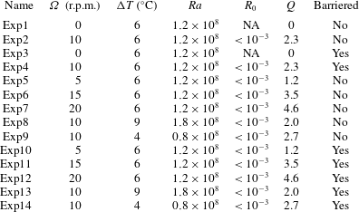
Experimental data and computed values for the non-dimensional parameters.
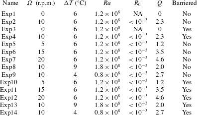
Since the main focus of the current study is the fundamental effects of rotation on HC, we chose to have
 $Q>1$
where rotation is believed to be important, but below values where baroclinic instability might emerge (
 $Q>O(5)$
). As listed in table 2, the experiments performed and investigated may be divided into two sets. In each set, the rotation rate
 $\unicode[STIX]{x1D6FA}$
and the base temperature difference
 $\unicode[STIX]{x0394}T$
were varied in such a way that
 $Q$
was changed from approximately
 $1$
to over
 $4$
, making it possible to analyse quantitatively effects of its magnitude on flow characters. In the first set, the domain is the axisymmetric annular gap. All experimental settings, including the boundary forcing, were axisymmetric, and so was the resulting flow. No instabilities were observed, probably because of the smallness of
 $Q$
and the axisymmetry of the boundary forcing (Sheard et al.
Reference Sheard, Hussam and Tsai2016) (figure 2). The experimental configurations in the second set were the same as those in the first one except that the axisymmetry broke down as a
 $4$
mm thick Plexiglas plate was mounted on the annulus base along a semi-radial plane. The plate acts as a full solid boundary, changing the annular gap into a closed basin. Effects of a closed geometry could therefore be studied through a comparison of the two sets.
A cylindrical polar coordinate system
 $(r,\unicode[STIX]{x1D703},z)$
was used in analysing results. The system has the origin located at the centre of the copper plate, the radial direction directed outwards from the origin, the azimuthal direction directed anti-clockwise when viewed from above and the polar axis directed upward from the base. For convenience, we sometimes used ‘zonal’ and ‘meridional’ to refer to azimuthal and radial directions.
Three-dimensional distribution of horizontal velocity and temperature were measured for all experiments. For velocity measurement, the horizontal light sheet created by Laser2 was traversed downward from the top to the bottom of the fluid and stopped every
 $2$
mm for a period of
 $5$
minutes. During this period,
 $1201$
images were taken by CCD2 at a sampling rate of
 $4$
Hz, yielding
 $1200$
instantaneous velocity fields.
For temperature measurements,
 $36$
radial sections were taken sequentially in
 $10^{\circ }$
increments of the polar angle. For each section, thermistor probes were traversed downward through holes in the lid and stopped every
 $2$
mm. At each depth, temperatures were measured at
 $16$
equally spaced radial locations between
 $r=25$
mm and
 $r=175$
mm in a period of
 $20$
s and at a sampling rate of
 $0.5$
Hz.
3 Experimental results
3.1 The establishment of circulation
Before settling down to an equilibrium state, the fluid experienced a transient stage. Evolution during that stage was believed to be sensitive to many factors such as the geometry of the tank, forcing, dissipation and initial and boundary conditions etc. (Mullarney et al. Reference Mullarney, Griffiths and Hughes2004; Wang & Huang Reference Wang and Huang2005). Hence the circulation during the transient period could be energetic with a pattern rather different from that of the steady state. For example, rested for a few hours after being filled in the tank, the working fluid initially had nearly uniform temperature, close to that of the environment. Shortly after the heating and cooling sources were turned on, the fluid right above the heating source achieved the highest temperature in the entire domain, forming convecting plumes that rose upward to the top of the fluid and inducing a fully penetrating overturning cell. The cell did not last long and was quickly replaced by a much lower cell as the fluid fed into the convecting region was continuously cooled.
The diffusion process determined an upper limit of the time scale for the system to reach a quasi-equilibrium state. According to the expression of the diffusion time
 $\unicode[STIX]{x1D70F}\sim H^{2}/\unicode[STIX]{x1D705}$
, the length of time for the current settings was approximately 40 h. The velocity field on a
 $r$
–
 $z$
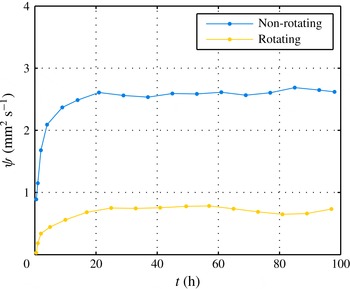
plane was measured every few hours from the onset of the experiment until over 100 h for Exp1 and Exp2. Defining the overturning streamfunction as the downward integration of the zonally averaged radial velocity
 $\bar{v}(r,z)$
 $$\begin{eqnarray}\unicode[STIX]{x1D713}(r,z)=\int _{z}^{H}\bar{v}(r,z)\,\text{d}z,\end{eqnarray}$$
we obtained its evolution over time as shown in figure 3. For both cases, the system reached a quasi-equilibrium state within 20–30 h, a time scale of the same order of magnitude but shorter than our estimate of the diffusion time. Based on this result and the estimate of
 $\unicode[STIX]{x1D70F}$
, all other experiments were run for over 50 h to make sure that the quasi-equilibrium state was reached.
3.2 Axisymmetric non-rotating and rotating HC
According to the well-accepted paradigm, as described in physical oceanography textbooks and in the literature (Thorpe Reference Thorpe2005; Lumpkin & Speer Reference Lumpkin and Speer2007; Talley et al. Reference Talley, Pickard, Emergy and Swift2011; Marshall & Speer Reference Marshall and Speer2012), the zonally averaged meridional overturning circulation is a global circulation cell wherein subtropical warm water is advected poleward at the surface; it then cools and sinks at high latitudes to form ‘deep’ and ‘bottom’ waters. These dense waters subsequently flow towards the equator below the thermocline at depth, cross isopycnals by mixing with lighter waters to return to the surface and eventually flow towards high latitudes to complete the cell. In somewhat of a contrast to the turbulent sinking motion occurring in confined polar regions, the upwelling takes place basin-wide in a relatively slow manner.
3.2.1 Non-rotating HC
Compared with the large-scale oceanic circulation described above, the circulation of the non-rotating HC was similar yet much simpler. For example, the flow had no azimuthal component and trajectories followed by fluid parcels were purely two-dimensional, on radial planes of constant
 $\unicode[STIX]{x1D703}$
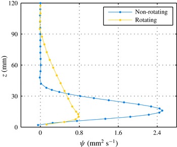
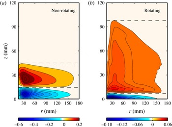
. The plot of the overturning streamfunction indicates a shallow overturning cell occupying only one-third of the total depth (figure 4) near the bottom. Three regions with obviously different radial flows existed in the vertical direction (as illustrated by dashed lines in figure 5): a quiescent upper region with vanishing overturning above
 $z=40$
mm, a thin bottom boundary layer with relatively strong inward velocity below approximately
 $z=15$
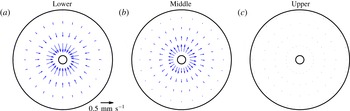
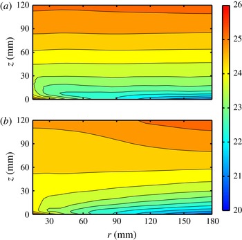
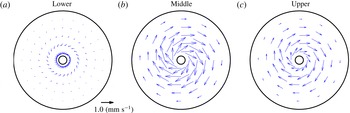
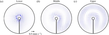
mm and a region in between with outward velocity (figures 5 and 6). Correspondingly, fluid parcels with lower temperature were advected towards the warmer part of the base within the boundary layer that was analogous to the oceanic thermocline (figure 7). They then entered an area of static instability above the warmer base and were fed into convecting plumes rising up along the inner wall. In the middle region water went outward and downward across isotherms, returning to the bottom to close the circulation loop.
Evolution of the overturning streamfunction at
 $r=60$
mm in time in the axisymmetric non-rotating case Exp1 (blue) and the axisymmetric rotating case Exp2 (yellow). The relative relation of the two curves is qualitatively similar at other radii.

Vertical distribution of the overturning streamfunction at radii
 $r=60$
mm in the axisymmetric non-rotating case Exp1 (blue) and the axisymmetric rotating case Exp2 (yellow).

Dynamically, we know the radial flows in the bottom boundary layer and in the interior, though in opposite directions, are both advective and driven by a radial pressure gradient (Mullarney et al. Reference Mullarney, Griffiths and Hughes2004; Hughes & Griffiths Reference Hughes and Griffiths2008). Both vertical components of the cell were diabatic. The rising component along the inner wall was forced by convective instability whereby potential energy was transferred to kinetic energy (Gayen, Griffiths & Hughes Reference Gayen, Griffiths and Hughes2014; Tsai et al. Reference Tsai, Hussam, Fouras and Sheard2016). The sinking motion was however driven by mixing primarily at the molecular scale. Ignoring the molecular diffusion, Sandström (Reference Sandström1908, Reference Sandström1916) hypothesized that without extra mechanical energy supporting diapycnal mixing, no persistent large-scale circulation can be maintained with the present geometry of the buoyancy forcing. On the other hand, the addition of mechanical stirring or mixing is able to significantly impact strength and structure of the circulation (Whitehead & Wang Reference Whitehead and Wang2008; Tailleux & Rouleau Reference Tailleux and Rouleau2010; Ilicak & Vallis Reference Ilicak and Vallis2012; Stewart Reference Stewart2012). Thus the diapycnal mixing can be terminal, acting as a choke point for the circulation. This is largely consistent with the popular hypothesis embraced by many in recent decades that the diapycnal mixing is crucial for the oceanic overturning circulation.
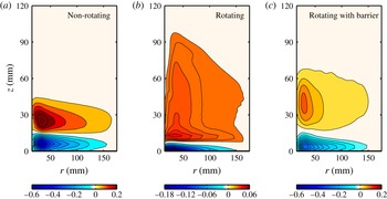
Distributions of the azimuthally averaged radial velocity (
 $\text{mm}~\text{s}^{-1}$
) in (a) the axisymmetric non-rotating case Exp1 and (b) the axisymmetric rotating case Exp2. Dashed lines in each figure schematically illustrate three regions with obviously different flow patterns, that is, an ‘upper’ region without mean radial velocity, a ‘middle’ region with outward (positive) radial velocity and a ‘lower’ region with inward (negative) radial velocity. It is important to note that these regions are defined by their distinctive flow patterns, rather than depth. So regions with the same name, ‘Upper’ for example, may not necessarily have the same depth ranges across different experiments.

Vectors of horizontal velocity averaged in three vertical regions in the axisymmetric non-rotating case Exp1, with ‘Lower’ denoting the bottom boundary layer with inward radial velocity, ‘Middle’ denoting the region with outward radial velocity and ‘Upper’ for the region above. The vector length legend is below panel (a) on the left.

3.2.2 Rotating HC
Introducing rotation caused noticeable changes to the zonally averaged stratification and overturning circulation (figures 4 and 7). First, the overturning cell was much weaker yet extended much higher from the bottom up to
 $z=100$
mm, with a greatly reduced radial velocity distributed more evenly in the vertical (figure 5). Second, isotherms were displaced in such a way that a bulge-like structure formed near the inner cylinder in the convecting region. Fundamental differences emerged as we further examined patterns of horizontal velocity in different regions. Most importantly, through the entire water column, the flow developed an azimuthal component in addition to the background rotation. This was because in presence of rotation, the radial pressure gradient generated by differential heating, instead of driving a radial flow, tended to support a relative azimuthal circulation as affected by the Coriolis force. Thus the circulation, originally along the
 $r$
–
 $z$
plane in the non-rotating case became three-dimensional.
Temperature distribution at quasi-equilibrium state in (a) the axisymmetric non-rotating case Exp1 and (b) the axisymmetric rotating case Exp2.

As illustrated in figure 8, in the bottom boundary layer, the flow was directed towards the warmer base but meanwhile turned cyclonically, as affected by the Coriolis force. From the boundary layer edge up to
 $z=100$
mm, the fluid circled around the inner wall anti-cyclonically, opposite to that in the boundary layer, due to a tendency to flow outward. Little radial component was observed although there was indeed some to support the weak overturning circulation. Above the overturning cell, the horizontal flow pattern looked almost the same as that in the middle region, but the azimuthally integrated radial transport was vanishingly small.
Vectors of horizontal velocity averaged in three vertical regions in the axisymmetric rotating case Exp2, with ‘Lower’ denoting the bottom boundary layer with inward radial velocity, ‘Middle’ denoting the region with outward radial velocity and ‘Upper’ for the region above. The vector length legend is below panel (a) on the left.

Potential vorticity is an important quantity that is related to the velocity and the stratification
 $\unicode[STIX]{x1D735}\unicode[STIX]{x1D70C}$
of the fluid. It is materially conserved when effects of non-conservative processes are absent, and satisfies (Pedlosky Reference Pedlosky1987)
 $$\begin{eqnarray}\boldsymbol{u}\boldsymbol{\cdot }\unicode[STIX]{x1D735}q=F,\end{eqnarray}$$
where time dependency has been dropped for the quasi-equilibrium state and
 $F$
denotes effects of unspecified sources or sinks such as diffusion and friction processes. We used Ertel’s formula to define PV,
 $$\begin{eqnarray}q\equiv \frac{(\unicode[STIX]{x1D74E}+2\unicode[STIX]{x1D734})}{\unicode[STIX]{x1D70C}}\boldsymbol{\cdot }\unicode[STIX]{x1D735}\unicode[STIX]{x1D70C},\end{eqnarray}$$
where
 $\unicode[STIX]{x1D74E}+2\unicode[STIX]{x1D734}$
is the absolute vorticity,
 $\unicode[STIX]{x1D74E}$
is the relative vorticity. The equation simply states that fluid parcels tend to move along PV contours and the cross-PV motion is allowed only when non-conservative processes exist. This theorem is at the core of classical theories of the wind-driven circulation such as Sverdrup balance (Sverdrup Reference Sverdrup1947) and the ventilated thermocline (Luyten, Pedlosky & Stommel Reference Luyten, Pedlosky and Stommel1983). It is also the backbone of probably the only well-known modern theory for the abyssal flow (Stommel Reference Stommel1958; Stommel, Arons & Faller Reference Stommel, Arons and Faller1958; Stommel & Arons Reference Stommel and Arons1960a
,Reference Stommel and Arons
b
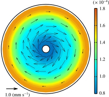
), but since then little progress has been made in its further application to the study of overturning circulation. In axisymmetric rotating experiments such as Exp2, PV contours were azimuthally aligned due to axisymmetry (figure 9), so away from the bottom boundary layer and the central convecting region where either friction or diabatic effects were relevant, flow to zero order was azimuthal, leaving the radial velocity that was mandatory for the overturning circulation to the next order with much smaller amplitude. In this sense, PV conservation imposed a severe constraint on the outward radial flow and hence the overturning circulation. As the outward motion of the interior flow was impeded by this constraint, fluid parcels carried upward by rising convective plumes tended to pile up next to the inner wall, causing the much deeper penetration depth of the circulation cell compared with their non-rotating counterparts.
Vectors of the isopycnal component of horizontal velocity superimposed on PV distribution on an isopycnal of the middle region where the azimuthally integrated radial flow is directed outward from the centre of the gap in the axisymmetric rotating experiment Exp2.

Since the horizontal velocity is of the order of
 $0.1$
mm s
 $^{-1}$
, the Rossby number
 $R_{0}\approx 3.0\times 10^{-4}$
and the zero-order flow was in geostrophy. Naturally one would argue that it was geostrophy instead of PV that constrained the overturning circulation, but we will show in the following experiments, that the role of PV variation is the decisive one.
3.2.3 Effects of a full radial barrier in the annulus
Experiments with an axisymmetric annulus are of limited relevance to oceanic overturning, except to those in the Antarctic Circumpolar Current and in the atmosphere. One reason is the lack of the effects of a closed geometry (Hignett et al.
Reference Hignett, Ibbetson and Killworth1981). With a radial barrier, the original axisymmetric annulus can be viewed as a
 $360^{\circ }$
wide sector, probably a closer match to the realistic ocean geometry compared with rectangular ones that were often adopted by previous HC studies (Rossby Reference Rossby1965; Speer & Whitehead Reference Speer and Whitehead1998; Park & Whitehead Reference Park and Whitehead1999; Wang & Huang Reference Wang and Huang2005). Moreover, interesting and important questions arise such as what the circulation pattern looks like, whether there exists advective radial flow along the wall, as suggested by Hignett et al. (Reference Hignett, Ibbetson and Killworth1981), and if so, what is its relation to the PV field?
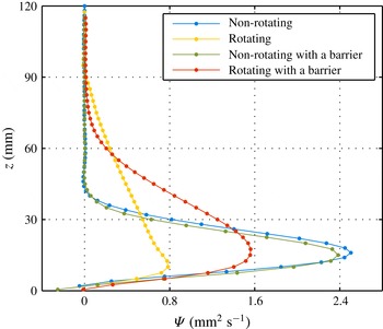
(i) Azimuthally averaged overturning circulation. Introducing a full radial barrier in the non-rotating situation only caused a slight decrease of the overturning streamfunction (figure 10), due to the viscosity exerted by the solid wall. In contrast, inserting a radial barrier in the rotating situation produced substantial changes and rendered to the flow a noticeable resemblance to that in the non-rotating situation. Instead of being distributed relatively homogeneously in the vertical above the boundary layer, the azimuthally averaged radial velocity showed a well-defined jet structure (figure 11), similar to those in the non-rotating situation yet with a weaker amplitude and higher vertical extent. As a result, the structure of the streamfunction indicated a much stronger but lower overturning cell (figure 10) compared with its axisymmetric counterpart. Therefore, inserting a radial barrier seemed to be able to eliminate effects of rotation, and how that happened will be closely examined in what follows.
Vertical distribution of the overturning streamfunction at radii
 $r=60$
mm in the axisymmetric non-rotating case Exp1 (blue), the axisymmetric rotating case Exp2 (yellow), the non-rotating barriered case Exp3 (green) and the rotating barriered case Exp4 (red).

Distributions of azimuthally averaged radial velocity (
 $\text{mm}~\text{s}^{-1}$
) in (a) the axisymmetric non-rotating case Exp1, (b) the axisymmetric rotating case Exp2 and (c) the rotating barriered case Exp4.

Vectors of horizontal velocity averaged in three vertical regions in the rotating barriered case Exp4, with ‘Lower’ denoting the bottom boundary layer with inward radial velocity, ‘Middle’ denoting the region with outward radial velocity and ‘Upper’ for the region above. The vector length legend is below panel (a) on the left.

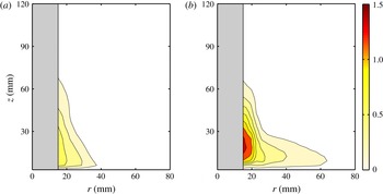
Distributions of vertical velocity ((
 $\text{mm}~\text{s}^{-1}$
), positive only) on two vertical sections which are parallel but facing each other on different sides of the radial barrier in Exp4, the rotating barriered case. Panel (a) is for the section near the western boundary where a strong radial current exists; panel (b) for that near the eastern boundary, if the domain is considered as a 360
 $^{\circ }$
wide pie-shaped sector with its northern boundary along the wall of the inner cylinder. Both sections are
 $5$
mm away from the barrier and extend only half way through the annulus, from the outer cylinder to the inner cylinder. The horizontal axis denotes distance to the centre of annulus.

(ii) Structure of velocity fields. As before, we divided the full depth into three regions of apparently different dynamics and examined the horizontal circulation in each of them. As shown in figure 12(a), in the bottom boundary layer, the general flow pattern was somewhat similar to the axisymmetric rotating case: flow was directed towards the centre of the cylinders to be heated and meanwhile turned anti-clockwise. Upon approaching the solid wall, fluid parcels with relatively high temperatures tended to be accumulated near the northeastern corner of the domain (if the annular gap with the barrier is considered as a pie-shaped sector, that is
 $360^{\circ }$
wide, and its northern boundary is along the wall of the inner cylinder), where more intense convection took place, as characterized by much stronger upward motion compared with other places along the entire northern boundary such as the western boundary (figure 13). At the top of convecting plumes that were formed along the northern boundary, fluid parcels became no more buoyant than their surroundings, moving outward and turning clockwise around the inner cylinder until they encountered the barrier on its eastern side (or the western boundary of the domain) (figure 12
b). They were then directed southward along the western boundary in a well-defined strong jet, turning anti-clockwise after meeting the southern boundary (the edge of the outer cylinder). Other than this radial jet, the flow in other regions was largely zonal, making small contribution to the overturning circulation. Furthermore, starting from the inner wall, the flow amplitude quickly weakened following the circulation path to nearly zero close to the eastern boundary. This tendency for continuous weakening of the horizontal motion indicated a divergence supporting more or less homogeneous downward motion in the interior and away from the central region, which supplied the northward mass flux observed in the bottom boundary layer. Above the middle region, the flow pattern was qualitatively similar to that below (figure 12
c), but had a very anti-symmetric structure about the barrier. In fact, the two opposing radial jets on the two sides of the wall were so anti-symmetric that the integration along the entire latitude was small, indicating the vanishing of the overturning circulation in this vertical range.
(iii) Potential vorticity. For axisymmetric (non-barriered) rotating experiments such as Exp2, we argued that the outward radial flow in the interior was severely constrained by zonally aligned PV barriers. In other words, in closing the overturning cell fluid parcels had to break the PV constraint before they had a chance to overcome the constraint of gravity and moved downward across isopycnals. In this regard, the PV constraint was a limiting factor for the overturning circulation. In rotating experiments with a radial barrier such as Exp4, outside the bottom boundary layer and the central convecting region, the relative vorticity was of the order of
 $10^{-4}$
, negligible compared with the planetary vorticity
 $f\equiv 2\unicode[STIX]{x1D6FA}$
(the ratio between the two is of the order of the Rossby number which was much smaller than 1), so according to (3.3), PV can be written as
 $$\begin{eqnarray}q\approx \frac{f}{\unicode[STIX]{x1D70C}}\frac{\unicode[STIX]{x2202}\unicode[STIX]{x1D70C}}{\unicode[STIX]{x2202}z},\end{eqnarray}$$
which is a function of the stratification.
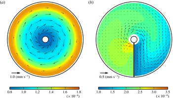
Vectors of the isopycnal component of horizontal velocity superimposed on PV distribution on an isopycnal of the middle region where the azimuthally integrated radial flow is directed outward from the centre of the gap in (a) the axisymmetric rotating case Exp2 and (b) the rotating barriered case Exp4.

Contrasting differences emerged as we compared side-by-side PV distributions of the two rotating experiments with and without the barrier (figure 14). Instead of being concentric, the PV contours, in the presence of the radial barrier, emanate from the inner cylinder without forming concentric closed contours, and terminate at the outer wall at an azimuthal angle similar to where they originate. Even though between the two zonal walls they turn first clockwise and then anti-clockwise in two azimuthal meanders, the pattern is still largely radial. Especially near the western boundary where the aforementioned strong jet was observed, the PV contours are entirely along the barrier, being meridional and parallel with the flow. A calculation of its vertical shear and horizontal density gradient confirmed the dominance of geostrophy (or thermal wind relation). Hence it is this particular pattern of PV distribution that functioned as a ‘conduit’, making it possible for a geostrophic flow to go southward, connecting the upwelling and downwelling stages with relatively little effort. If the previous axisymmetric rotating experiment was regarded as an example of PV exerting a constraint on the overturning circulation, the current case is a perfect one of PV removing its barrier and allowing for a southward flow. This was possible because of the presence of a closed geometry, against the western boundary of which the flow adjusted itself to develop a zonal pressure gradient to support the large-scale geostrophic flow.
(iv) Dependence on
 $Q$
. As
 $Q$
changes from approximately
 $1$
to over
 $4$
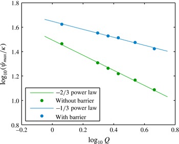
, the rotating non-barriered experiments (Exp2, Exp5–Exp9) are qualitatively similar to each other in basic flow patterns, and those barriered experiments (Exp4, Exp10–Exp14) also bear strong resemblance. The two sets, however, are dramatically different, due to the effects of the closed geometry. Furthermore, the peak value of
 $\unicode[STIX]{x1D713}$
in the non-barriered cases is scaled as
 $Q^{-2/3}$
, but its dependence on
 $Q$
in the barriered cases is notably weaker, with only a power of
 $-1/3$
(figure 15). Obviously, the influence of the closed geometry is crucial for rotating HC but is not covered by the existing theoretical framework including the hypothesis of
 $Q$
. One therefore needs to be more careful in applying this parameter to consideration of geophysical problems such as the large-scale oceanic overturning circulation.
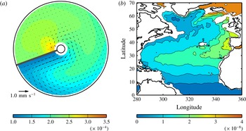
(v) Discussion. As a striking feature of the flow in the presence of a radial barrier, the strong current along the western boundary is reminiscent of the ‘Deep Western Boundary Current’ (DWBC) (Hogg Reference Hogg1983; Pickart Reference Pickart1992) in the North Atlantic basin, since both are closely related to the overturning circulation (or thermohaline circulation) and directed away from the region of deep water formation. Even with these apparent similarities, it is still a formidable challenge to establish any analogy between the two, since the oceanic situation differs from laboratory experiments in so many aspects such as the existence of the background PV gradient, and quite different values of those important parameters defined in § 2.2. However, the general patterns of PV distribution of the two are surprisingly similar (figure 16): contours of both are largely meridional, connecting the cooling and heating regions, and are closely aligned with the solid wall near the western boundary. Presumably, the realistic DWBC in this region is also dynamically similar to that in our experiments, being geostrophic in nature. The conjecture that the DWBC, or at least part of it, is aligned with PV contours and in geostrophic balance is different from the conventional wisdom, according to which the western boundary currents are directed across background PV contours and friction processes are crucial for their dynamical balance (Pedlosky Reference Pedlosky1987).
Dependence of
 $\unicode[STIX]{x1D713}_{max}/\unicode[STIX]{x1D705}$
on the parameter
 $Q$
in non-barriered (green) and barriered (blue) cases.

(a) The same as figure 14(b), but rotated
 $70^{\circ }$
clockwise. (b) Distribution of the mean PV (calculated as
 $-f\unicode[STIX]{x2202}\unicode[STIX]{x1D70C}/\unicode[STIX]{x2202}z$
) on the mean potential density surface
 $\unicode[STIX]{x1D70E}_{2}=36.895~\text{kg}~\text{m}^{-3}$
in the North Atlantic basin, calculated using the US Navy Generalized Digital Environment Model (GDEMVersion 3.0) annual mean climatology of observed temperature and salinity fields. Data sources are described by Wang et al. (Reference Wang, Xie, Q and Huang2011).

4 Summary and discussion
Much of the long-standing debate regarding what controls the overturning circulation has been mostly concerned with differential buoyancy forcing at the surface and diapycnal mixing in the interior, especially the latter, which, from the energetic point of view, was recognized as crucial in determining the overturning circulation. In the current study however, we want to remind the reader that besides diapycnal mixing, the theorem of PV conservation is also very important for overturning circulation by putting a strong constraint on the meridional component of the circulation in the ocean interior. As required by this rule, the isopycnal component of the flow to zero order is along PV contours except that the effects of non-conservative processes such as friction and diffusion are strong enough to break the PV constraint.
In the current study, the two sets of rotating experiments, the non-barriered and barriered cases, have exactly the same external parameters such as axisymmetric distribution of base temperature, viscosity and diffusivity, but their differences are remarkable simply because the insertion of a radial barrier dramatically changed the relationship between the meridional flow and PV distribution. In the non-barriered experiments, since the distribution of PV is axisymmetric without any zonal variation, any flow in the radial direction has to overcome the PV constraint, as affected by friction, leading to the small amplitude of the overturning circulation. Once a full radial barrier was introduced, the flow equilibrated towards a state where PV contours were radially aligned within a sub-region near the western boundary. Through this conduit, fluid parcels were carried more readily southward, leading to a substantial strengthening of the overturning circulation. Apparently, the theorem of PV conservation imposed a strong constraint over the circulation, and under certain circumstances, it could be a limiting factor, prohibiting the meridional flow and hence the overturning cell.
This is not the first time that PV conservation has been considered in respect of overturning circulation, but little speculation has been made about its role in the overall picture of the circulation relative to other ingredients such as differential buoyancy forcing and diapycnal mixing. Probably the first dynamical theory of the abyssal circulation, developed through a series of papers by Stommel and his collaborators (Stommel Reference Stommel1958; Stommel et al. Reference Stommel, Arons and Faller1958; Stommel & Arons Reference Stommel and Arons1960a ,Reference Stommel and Arons b ), is a straightforward application of Sverdrup theory, which, in essence, is about PV conservation. However, diapycnal mixing was not explicitly considered: its effect was only crudely represented by the stretching of vortex tubes in a barotropic fluid. Thus to what extent their theory would be relevant for the real ocean remains an open question.
With the above having been said, we believe that the PV distribution is central in shaping the overturning circulation but not much attention has been paid to the subject in recent years. It should be noted that although our experimental results disclosed some essential facts, their direct applicability to the real ocean is probably limited, due to ignorance of many complicating factors. First, a PV gradient that is independent of circulation, such as the topographic and planetary
 $\unicode[STIX]{x1D6FD}$
, was not considered. The effect of the former on the overturning is currently being investigated with laboratory experiments, but as to the planetary
 $\unicode[STIX]{x1D6FD}$
, numerical models are probably necessary. Second, effects of waves and eddies resulting from instabilities were not considered. Geostrophic eddies are a ubiquitous feature of the ocean, and are believed to be able to induce strong along-isopycnal mixing of various properties such as temperature, salinity and PV. However, many relevant issues regarding eddies and their effects remain unclear. For example, what the overturning circulation is like if the rotating annular gap is seeded with turbulent eddies, an analogy to the Antarctic Circumpolar Current. Will they allow the meridional flow to zero order by eroding the PV gradient or act as an external forcing, driving fluid across PV contours? Answers to these questions await further studies with laboratory or numerical experiments in the future.
Acknowledgements
This work was supported by the National Basic Research Priorities Program of China through grant 2015CB954300 and the National Natural Science Foundation of China under grants 41376011 and 41276014. The authors would like to thank the anonymous reviewers for their valuable suggestions.