1. Introduction
Water entry and exit of objects can create cavities in a fluid, see Birkhoff (Reference Birkhoff and Zarantonello1957). Real-life examples include water entry of projectiles, water exit of underwater vehicles and TNT (trinitrotoluene) explosions near a water surface, see Truscott, Epps & Belden (Reference Truscott, Epps and Belden2014). A depression on the water’s surface, followed by its collapse, can be generated by high-speed vessels with transom sterns. Martinez-Legazpi et al. (Reference Martìnez-Legazpi, Korobkin and Lasheras2015) studied the early-time evolution of such depressions for a rectangular stern using the ‘two-dimensions-plus-time’ approach. The depression behind the stern collapses under gravity, leading to the formation of so-called corner waves. These waves propagate toward the centre of the wake and collide there, producing the so-called rooster tail, which significantly contributes to flow aeration in the vessel’s wake.
Sketch of the problem at
 $t'=0$
.

In this paper, short-time behaviour of a two-dimensional flow caused by the collapse of a wedge-shaped cavity on a water free surface is investigated, see figure 1, where
 $g$
is the gravitational acceleration acting along the negative
 $y$
-axis. The liquid is assumed to be inviscid and incompressible, and the flow induced by the collapse of the depression is taken to be potential. The depression is symmetric in the present study. The distance
 $h_1$
from the cavity vertex to the bottom is smaller than the total water depth
 $h_2$
. No motion occurs when
 $h_1=h_2$
. When
 $h_1=0$
, the problem reduces to a dam-break scenario with a rigid vertical wall in front of an inclined initial free surface. It is shown in this paper that the ratio
 $\delta =h_1/h_2$
determines the strength of the singularity in the global leading-order flow at the depression vertex. To the best of the authors’ knowledge, the flow resulting from the collapse of a wedge-shaped depression has not been previously studied.
The flow caused by a cavity collapse is of interest in several applications. Khanga et al. (Reference Khangaonkar and LeMehaute1992) studied cylindrical cavity collapse on a dry sea bed. They wrote that such a cavity can be caused by ‘…explosions performed in shallow lagoons, or ponds, and nuclear explosions carried out on the continental shelf. It would also be the case of water waves generated by the fall of a large meteorite in the ocean, an event which some researchers claim to have occurred some 65 million years ago’. They noticed that ‘this collapse is similar to the dam-break problem on a dry bed’. The problem was solved for large times using the shallow water equations and the method of characteristics. The water waves generated by the cavity collapse were computed. The obtained results were suggested to be used to estimate the initial size of the cavity and the source of the cavity using measurements of the waves at a distance from the cavity. Another application concerns high-speed vessels with transom sterns. Martinez-Legazpi et al. (Reference Martìnez-Legazpi, Korobkin and Lasheras2015) studied the latter problem for a rectangular stern using the ‘two-dimension-plus-time’ approach. The depression in the water’s surface behind the stern collapses due to gravity with the formation of so-called corner waves. The corner waves propagate towards the cavity centre and collide there, making the so-called rooster tail, which significantly contributes to the flow aeration in the wake of the vessel. The cavity collapse problem is linked to the jet formation in bubbles bursting at a free surface, see Duchemin et al. (Reference Duchemin, Popinet, Josserand and Zaleski2002). In this numerical investigation, it is argued that, for some parameter values, the jet formation, which is inertia dominated, is similar to a singular flow that is caused by the collapse of a conical cavity. More applications are reported by Zeff et al. (Reference Zeff, Kleber, Fineberg and Lathrop2000). In this theoretical and experimental investigation, experiments are carried out to show that surface singularities are formed ‘by the collapsing depressions of standing waves’. Recently, Gordillo et al. (Reference Gordillo and Blanco-Rodríguez2023) introduced a ‘theory of the jets after the initial collapse of cavities with applications to the bubble bursting jets’. It is argued that their results are applicable to the very fast jets ‘produced after a bubble cavitates very close to a wall’ and to ‘the quantification of the so-called bazooka effect’.
The flow due to symmetric wedge cavity collapse can be thought as a dam-break flow with the vertical wall at the line of symmetry and a part of the free surface, being initially inclined. The flow can also be considered as that caused by instant removal of a rigid wedge floating on the free surface. Initially, at
 $t=0^-$
, there is no flow and the pressure in the fluid is hydrostatic. When the wedge is suddenly removed, at
 $t=0^+$
, the gravity-driven flow starts as the cavity is filled by the surrounding fluid. From the experimental and theoretical investigations of dam-break problems (Stansby, Chegini & Barnes Reference Stansby, Chegini and Barnes1998; Korobkin et al. Reference Korobkin and Yilmaz2009; Yilmaz, Korobkin & Iafrati Reference Yilmaz, Korobkin and Iafrati2013) the leading-order flow singularities are expected at the corner points of the free surfaces or where a fluid meets a rigid surface (for the dry-bed dam-break problem). It will be shown that the flow velocity is singular at the leading order of small times at the vertex of the wedge cavity.
Initial dam breaking flows can be considered as a class of nonlinear Cauchy–Poisson flows released from rest, see Tyvand (Reference Tyvand2020). Cauchy–Poisson flows are defined as flows with an initial free-surface elevation, released from rest to flow freely under gravity. Both infinite and finite-depth problems were investigated by Tyvand (Reference Tyvand2020). It was concluded that ‘the influence of the bottom is remarkably small on the surface flow field with maximum amplitude’. Tyvand, Mulstand & Bestehorn (Reference Tyvand, Mulstand and Bestehorn2021) investigated a nonlinear Cauchy–Poisson problem with impulsive free-surface forcing analytically and numerically. A small-time expansion of the fully nonlinear free-surface flow has been carried out exactly to third order. In both investigations of Tyvand (Reference Tyvand2020) and Tyvand et al. (Reference Tyvand, Mulstand and Bestehorn2021), there are no singularities at the free surface unlike in the present study, because the initial disturbances of the free surface in Tyvand (Reference Tyvand2020) and Tyvand et al. (Reference Tyvand, Mulstand and Bestehorn2021) are smooth.
The short-time behaviour of a three-dimensional cavity collapse flow was studied by Fetahu, Yaman & Yilmaz (Reference Fetahu, Yaman and Yilmaz2022), where the cavity was in the shape of a vertical cylinder starting at the rigid bed and extending all the way to the free surface. It was concluded that the leading-order flow singularity at the intersection line between the rigid bottom and the cavity free surface is logarithmic, similar to the classical two-dimensional dam-break problem and that three-dimensional effects are important when the radius of the cavity is small compared with the fluid height. Large-time behaviour of the same problem was studied by Khanga et al. (Reference Khangaonkar and LeMehaute1992) by using the nonlinear long-wave equations and the method of characteristics. They claimed that their method simulates the generation and collapse of water craters created by explosions in shallow water.
Martinez-Legazpi et al. (Reference Martìnez-Legazpi, Korobkin and Lasheras2015) investigated the pattern of corner waves formed in the wake of high-speed ships with transom sterns. The corner waves are responsible for air/water mixing in the wake, which makes the wake as well as the ship’s path visible for a long time. For short distances from the stern, the problem near the corner points was converted to a dam-break problem with a wet basin. Using matched asymptotic expansions, the flow near the corner was described for short distances from the stern, which is equivalent to short times in our formulation. Numerical computations were performed using a boundary element method, which showed mushroom-shaped jet formation at the corner points. This was found first for the wet dam break Stansby et al. (Reference Stansby, Chegini and Barnes1998). The present problem is similar to that of Martinez-Legazpi et al. (Reference Martìnez-Legazpi, Korobkin and Lasheras2015) in the leading order, with the only difference between the two problems being the initial cavity shape.
The formulation of the problem and the short-time expansions of the velocity potential and the free-surface displacement are presented in § 2. In § 3, the leading-order boundary-value problem is solved by conformal mapping and the singular behaviour of the flow at the corner points is analysed. The flow velocities and the free-surface shapes are presented in § 4 and compared with the numerical solution by OpenFOAM. The boundary-value problem describing the local flow near the wedge cavity vertex is formulated in § 5. Finally, conclusions are drawn in § 6.
2. Formulation of the problem
A two-dimensional gravity-driven flow generated when a rigid wedge floating on a liquid free surface is suddenly removed is investigated, see figure 1. The depth of the liquid is
 $h_2$
and the distance of the wedge vertex from the bottom is
 $h_1$
,
 $0\lt h_1\lt h_2$
. Initial shape of the flow region is symmetric in the present study. Note that the horizontal dimension of the wetted part of the wedge is selected to be double the water depth. We focus on a simple non-smooth configuration here to explain the method of analysis of gravity-driven problems for short times. More complex symmetric and asymmetric cases can be studied using the same methods as in the present investigation, but calculations will be more elaborate.
The problem of the gravity-driven flow is considered in the Cartesian coordinate system
 $Ox'y'$
, where
 $y'=0$
corresponds to the liquid bottom and
 $x'=0$
corresponds to the vertical line of the flow symmetry. The liquid is assumed to be inviscid and incompressible. Throughout the paper, a prime stands for dimensional variables. Initially, the liquid is at rest. The gravity-generated flow is assumed to be potential flow and symmetric with respect to
 $x'=0$
. The free surface for
 $t'\gt 0$
consists of two parts: the initially horizontal part
 ${\textit{FS}}_{h}^{\prime}(t')$
, and the initially wedge-shaped part
 ${\textit{FS}}_{v}^{\prime}(t')$
 \begin{align}{\textit{FS}}_{h}^{\prime}(t') = \left \{(x',y',t') \,:\,y'= h_2 + {\eta}_{v}^{\prime}(x',t'),\,|x'|\gt h_2 \right \},\end{align}
 \begin{align}{\textit{FS}}_{v}^{\prime}(t') = \left \{(x',y',t') \,:\,y'=h_1+\frac {h_2-h_1}{h_2}|x'| + {\eta}_{d}^{\prime}(x',t'),\,|x'|\lt h_2 \right \},\end{align}
where
 ${\eta}_{d}^{\prime}(x',t')$
is the vertical displacement of the initially wedge-shaped free surface and
 ${\eta}_{v}^{\prime}(x',t')$
is the vertical displacement of the initially horizontal free surface. The functions
 ${\eta}_{d}^{\prime}(x',t')$
and
 ${\eta}_{v}^{\prime}(x',t')$
are even functions of
 $x'$
. The free surface is continuous at each time instant, in particular
 ${\eta}_{d}^{\prime}(h_2,t')={\eta}_{v}^{\prime}(h_2,t')$
, but its slope can be discontinuous there. Initially
 ${\eta}_{d}^{\prime}(x',0)=0$
and
 ${\eta}_{v}^{\prime}(x',0)=0$
.
The flow is described by the velocity potential
 $\varphi '(x',y',t')$
that satisfies the following initial-boundary-value problem:
 \begin{align}{\nabla} ^2 \varphi ' = 0\quad \text{in} \quad \varOmega '(t'),\end{align}
 \begin{align}p' =p_{atm}\quad &\text{on} \quad {\textit{FS}}'(t'),\end{align}
 \begin{align}\frac {\partial \varphi '}{\partial y'} -sgn(x')\frac {h_2-h_1}{h_2}\frac {\partial \varphi '}{\partial x'}-\frac {\partial \varphi '}{\partial x'} \frac {\partial {\eta}_{d}^{\prime}}{\partial x'}-\frac {\partial {\eta}_{d}^{\prime}}{\partial t'} &=0\quad \text{on} \quad {\textit{FS}}_{v}^{\prime}(t'),\end{align}
 \begin{align}\frac {\partial \varphi '}{\partial y'}- \frac {\partial \varphi '}{\partial x'}\frac {\partial {\eta}_{v}^{\prime}}{\partial x'}-\frac {\partial {\eta}_{v}^{\prime}}{\partial t'} &=0\quad \text{on} \quad {\textit{FS}}_{h}^{\prime}(t'),\end{align}
 \begin{align}\frac {\partial \varphi '}{\partial y'} &=0 \quad \text{at} \quad y' = 0,\end{align}
 \begin{align}\varphi ' \rightarrow 0, \quad {\eta}_{v}^{\prime}(x',t')\rightarrow 0 & \quad \text{as} \quad x' \rightarrow \mp \infty,\end{align}
 \begin{align}\varphi '(x',y',0)=0,\, {\eta}_{v}^{\prime}(x',0) &=0,\, {\eta}_{d}^{\prime}(x',0)=0,\end{align}
where
 $sgn(x')=1$
for
 $x'\gt 0$
and
 $sgn(x')=-1$
for
 $x'\lt 0$
,
 $\varOmega '(t')$
is the flow region bounded by the free surfaces,
 $FS'(t')= {\textit{FS}}_{h}^{\prime}(t') \cup {\textit{FS}}_{v}^{\prime}(t')$
and the bottom
 $y'=0$
,
 $p_{atm}$
is the atmospheric pressure above the liquid and
 $p'$
is the hydrodynamic pressure related to the velocity potential by Bernoulli’s equation
 \begin{eqnarray} \frac {p'}{\rho _0}+\frac {\partial \varphi '}{\partial t'}+\frac {1}{2}|\boldsymbol{\nabla }\varphi '|^2+g(y'-h_2)+q(t')=\frac {p_{atm}}{\rho _0}, \end{eqnarray}
where
 $\rho _0$
is the liquid density and
 $g$
is the gravitational acceleration. The conditions in the far field (2.8) and the dynamic condition (2.4) on the free surface provide
 $q(t')=0$
. Equations (2.5) and (2.6) are the kinematic boundary conditions at the free surface. They imply that fluid particles on the surface stay there at any time instant
 $t'\geqslant 0$
. Equation (2.7) is the slip boundary condition at the rigid bottom. The initial conditions (2.9) imply that initially the fluid is at rest. Bernoulli’s equation (2.10) and the initial conditions (2.9) yield that the fluid pressure is hydrostatic initially. It is convenient to introduce dimensionless variables, which are denoted with the same symbols but without a prime
 \begin{align}x' = h_2 x,\quad y'= h_2 y,\quad t'=Tt, \quad \delta =h_1/ h_2,\end{align}
 \begin{align}\varphi ' = g h_2 T \varphi ,\quad p'=\rho _0gh_2 p,\quad {\eta}_{d}^{\prime}= \varepsilon h_2 \eta _d,\quad {\eta}_{v}^{\prime}=\varepsilon h_2 \eta _v\end{align}
where
 $\textrm{T}$
is a suitable time scale,
 $0\lt \delta \lt 1$
and
 $\varepsilon = gT^2/h_2$
is a small dimensionless parameter. The parameter
 $\varepsilon$
is introduced in order to indicate that we are concerned with the initial stage of the flow.
The problem (2.3)–(2.9) reads in the dimensionless variables
 \begin{align}{\nabla} ^2 \varphi =0\quad \text{in} \quad \varOmega (t),\end{align}
 \begin{align}\frac {\partial \varphi }{\partial t} + \frac {1}{2}\varepsilon |\boldsymbol{\nabla }\varphi |^2 +y-1=0 \quad \text{on} \quad {\textit{FS}}(t),\end{align}
 \begin{align}\frac {\partial \varphi }{\partial y} -sgn(x)(1-\delta )\frac {\partial \varphi }{\partial x}-\varepsilon \frac {\partial \varphi }{\partial x} \frac {\partial \eta _d}{\partial x}-\frac {\partial \eta _d}{\partial t}=0\quad \text{on} \quad {\textit{FS}}_v(t),\end{align}
 \begin{align}\frac {\partial \varphi }{\partial y}-\varepsilon \frac {\partial \varphi }{\partial x}\frac {\partial \eta _v}{\partial x}-\frac {\partial \eta _v}{\partial t}=0\quad \text{on} \quad {\textit{FS}}_h(t),\end{align}
 \begin{align}\frac {\partial \varphi }{\partial y}=0 \quad \text{at} \quad y=0,\end{align}
 \begin{align}\varphi \rightarrow 0,\quad \eta _v(x,t)\rightarrow 0 \quad \text{as} \quad x \rightarrow \mp \infty,\end{align}
 \begin{align}\varphi (x,y,0)=0,\, \eta _v(x,0)=0,\, \eta _d(x,0)=0,\end{align}
where
 $ {\textit{FS}}(t)$
is the union of the free surfaces
 $FS_h(t)$
and
 $FS_v(t)$
 \begin{align} {\textit{FS}}_h(t)&= \left \{(x,y,t):\, y= 1+\varepsilon \eta _v(x,t) ,\, |x|\gt 1\right \}, \end{align}
 \begin{align} {\textit{FS}}_v(t)&= \left \{(x,y,t):\,y=\delta +(1-\delta )|x|+\varepsilon \eta _d(x,t),\,|x|\lt 1 \right \}. \end{align}
At
 $t=0$
, (2.20) and (2.21) become
 \begin{align} {\textit{FS}}_h(0)&= \{(x,y,0)\big |\, y= 1 ,\, |x|\gt 1\}, \end{align}
 \begin{align} {\textit{FS}}_v(0)&= \{(x,y,0)\big |\,y=\delta +(1-\delta )|x|,\, |x|\lt 1\}. \\[9pt] \nonumber \end{align}
The velocity potential and the free-surface elevations are sought in the form
 \begin{align} \varphi (x,y,t,\varepsilon ) &= \hat {\varphi }_0(x,y,t) + \varepsilon \hat {\varphi }_1(x,y,t) + \textit {O}(\varepsilon ^2),\nonumber \\ \eta _v(x,t,\varepsilon ) &= \hat {\eta }_{v0} (x,t) + \varepsilon \hat {\eta }_{v1} (x,t) + \textit {O}(\varepsilon ^2),\nonumber \\ \eta _d(x,t,\varepsilon ) &= \hat {\eta }_{d0} (x,t) + \varepsilon \hat {\eta }_{d1} (x,t) + \textit {O}(\varepsilon ^2), \end{align}
as
 $\varepsilon \rightarrow 0$
. Substituting asymptotic formulae (2.24) in (2.13)–(2.19), using the Taylor expansions of the boundary conditions (2.14)–(2.16) around the initial position of the free surface and collecting terms with the same powers of
 $\varepsilon$
, we arrive at the boundary-value problems for the functions
 $\hat {\varphi }_j(x,y,t)$
,
 $\hat {\eta }_{vj}(x,t)$
,
 $\hat {\eta }_{dj}(x,t)$
. The corresponding boundary-value problems,
 $j\geqslant 0$
, can be solved one after another starting from the leading-order problem with
 $j=0$
.
3. The leading-order flow
The boundary-value problem for the leading-order solution is obtained from (2.13)–(2.19) by setting
 $\varepsilon =0$
 \begin{align}{\nabla} ^2 \hat {\varphi }_0 &= 0\quad \text{in} \quad \varOmega (0),\end{align}
 \begin{align}\hat {\varphi }_0 &= 0 \quad \text{at}\quad\, y=1, \,|x|\gt 1,\end{align}
 \begin{align}\hat {\varphi }_0= t(1-y) \quad \text{at} \quad & y=\delta +(1-\delta )|x|,\,|x|\lt 1,\end{align}
 \begin{align}\frac {\partial \hat {\varphi }_0}{\partial y} - sgn(x)(1-\delta )\frac {\partial \hat {\varphi }_0}{\partial x} -\frac {\partial \hat {\eta _{d0}}}{\partial t} =0 &\quad \text{at}\quad y=\delta +(1-\delta )|x|,\,|x|\lt 1,\end{align}
 \begin{align}\frac {\partial \hat {\varphi }_0}{\partial y} - \frac {\partial \hat {\eta }_{v0}}{\partial t} =0 \quad &\text{at}\quad y=1,\, |x|\gt 1,\end{align}
 \begin{align}\frac {\partial \hat {\varphi }_0}{\partial y}=0 \quad &\text{at}\quad y=0,\quad -\infty \lt x\lt \infty ,\end{align}
 \begin{align}\hat {\varphi }_0(x,y,t) \rightarrow 0,\quad \hat {\eta }_{v0}(x,t)\rightarrow 0 \quad &\text{as} \quad x\rightarrow \mp \infty,\end{align}
 \begin{align}\hat {\varphi }_0(x,y,0)=0,\, \hat {\eta }_{v0}(x,0) &= 0,\, \hat {\eta }_{d0}(x,0)=0.\end{align}
The dynamic boundary condition (2.14) provides, at the leading order,
 $\partial \hat {\varphi }_0/\partial t+y-1=0$
on the free surface
 $FS(0)$
. Integrating this condition with respect to time we obtain
 $\hat {\varphi _0}+yt-t=\text{constant},$
where the constant is zero when accounting for the initial conditions (2.19), we arrive at the boundary conditions (3.2) and (3.3). Equations (3.1)–(3.8) show that the time
 $t$
can be separated in such a way that
 $\hat {\varphi }_0(x,y,t)=t\varphi _0(x,y)$
,
 $\hat {\eta }_d(x,t)=({1}/{2})t^2\eta _d(x)$
,
 $\hat {\eta }_v(x,t)=({1}/{2})t^2\eta _v(x)$
, where the new unknown functions
 $\varphi (x,y)$
,
 $\eta _d(x)$
and
 $\eta _v(x)$
depend on the single dimensionless parameter
 $\delta$
,
 $0\leqslant \delta \leqslant 1$
, see figure 2. The function
 $\varphi _0(x,y)$
is the leading-order acceleration potential of the initial flow. The velocity potential is continuous along the free surface, including the corner points D, E and F, as it follows from the boundary conditions (3.2) and (3.3). However, the flow velocity could be discontinuous at these corner points within the present approximation.
Sketch of the leading-order boundary-value problem.

We shall determine the structures of the local flows near the corner points
 $\textrm{E}$
and
 $\textrm{F}$
before solving the leading-order problem (3.1)–(3.8), see the encircled regions in figure 3.
Local problems around the corner points
 $\textrm{E}(0,\delta )$
and
 $\textrm{F}(1,1)$
.

First, the flow in a small vicinity of the vertex point
 $\textrm{E}$
is analysed. The local Cartesian
 $(\tilde {x},\tilde {y})$
and polar
 $(\tilde {r},\tilde {\theta })$
coordinates near the corner point
 $\textrm{E}$
are introduced by
 \begin{align} x &= \tilde {x}=\tilde {r}\cos {\tilde {\theta }}, \end{align}
 \begin{align} y &= \tilde {y}+\delta =\tilde {r}\sin {\tilde {\theta }}+\delta , \\[9pt] \nonumber \end{align}
where
 $\tilde {r}\gt 0$
,
 $\tilde {r}\ll 1$
and
 $-\pi -\alpha \lt \tilde {\theta }\lt \alpha$
, see figure 3(a), and
 $\alpha$
is the angle between the right inclined part of the wedge cavity
 $EF$
and the horizontal line,
 $\alpha =\arctan (1-\delta )$
and
 $0\lt \alpha \lt \pi /4$
. There are two boundary conditions to be satisfied by the local flow on the free surface near the corner point
 $\textrm{E}$
 \begin{eqnarray} \varphi _0(\tilde {x},\tilde {y}) = 1-(\delta +\tilde {y})=(1-\delta )(1-|\tilde {x}|)\,\, \text{on}\,\,\tilde {\theta }=\alpha \, \text{and}\,\,\tilde {\theta }=-\pi -\alpha . \end{eqnarray}
The local solution of the Laplace equation in the region
 $-\pi -\alpha \lt \tilde {\theta }\lt \alpha$
,
 $\tilde {r} \ll 1$
subject to the boundary conditions (3.11) is obtained by separation of variables
 \begin{eqnarray} \varphi _0(\tilde {x},\tilde {y})=(1-\delta -\tilde {y})+C_1\tilde {r}^{\gamma }\sin \big [\gamma (\tilde {\theta }-\alpha )\big]+o(\tilde {r}^\gamma ), \end{eqnarray}
where
 $\gamma =\pi / (\pi + 2\alpha )$
and
 $C_1$
is a constant which can be determined by using the complete solution of the problem (3.1)–(3.8), see Appendix A.
The singular nature of the flow depends on the angle
 $\alpha$
. As
 $\alpha \to (\pi /4)^-$
, which corresponds to a right-angled symmetric wedge-shaped cavity,
 $\delta \to 0^+$
, the singularity of the flow velocity is of the order
 $\textit {O}(\tilde {r}^{-1/3})$
as
 $\tilde {r}\rightarrow 0$
. At the other extreme, as
 $\alpha \to 0^+$
and
 $\delta \to 1$
, which is the case that there is no cavity and the flow domain is a horizontal infinite strip, we have
 $\gamma -1=0$
and there is no singularity of the velocity field at
 $\textrm{E}$
. This type of a power-law singularity of the leading-order short-time flow velocity,
 $\textit {O}(\tilde {r}^{-1/3})$
as
 $\tilde {r}\rightarrow 0$
, is known as a power-singular velocity. A power-singular velocity of leading-order short-time flows is typical for some dam-break and impact problems (see Yilmaz et al. Reference Yilmaz, Korobkin and Iafrati2013; Fetahu et al. Reference Fetahu, Yaman and Yilmaz2022; Korobkin et al. Reference Korobkin and Yilmaz2023). Yilmaz et al. (Reference Yilmaz, Korobkin and Iafrati2013) investigated initial stages of a dam-break problem involving two fluids of differing heights on either side of a dam. One of the conclusions of that paper is that, when the fluids are of the same density, the leading-order flow singularity at the triple point, where the free surfaces of the fluids and the interface meet, is of the order of
 $\tilde {r}^{-1/3}$
, using the same notation as in this paper. The same singular behaviour in both cases is not a coincidence. In fact, the dam-break problem studied in Yilmaz et al. (Reference Yilmaz, Korobkin and Iafrati2013) can be considered as an asymmetric, right-angled wedge-shaped cavity collapse problem which can be obtained from the present symmetric wedge problem by a rotation of an angle
 $\alpha$
in the counter-clockwise direction. Note that the symmetric and asymmetric wedge-shaped cavity collapse problems have the same singular flow behaviour at the leading order. The local analysis of the flow at the leading order implies that the solution of the problem (3.1)–(3.8) should be considered as the outer solution valid outside a small vicinity of the corner point
 $\textrm{E}$
. In a close proximity of this corner point, an inner problem should be formulated for
 $\varepsilon \rightarrow 0$
. The dimension of the vicinity tends to zero as
 $\varepsilon \rightarrow 0$
. It will be shown in § 5 below that the local flow is nonlinear and self-similar. The inner solution describes the flow with bounded velocities.
The local flow around the corner point
 $\textrm{F}$
(the vicinity of the corner point
 $\textrm{D}$
is considered in a similar way) is described in the local Cartesian
 $(\overline {x},\overline {y})$
and polar
 $(\overline {r},\overline {\theta })$
coordinates is defined by
 \begin{align} x &= \overline {x}+1=\overline {r}\cos {\overline {\theta }}+1, \end{align}
 \begin{align} y &= \overline {y}+1=\overline {r}\sin {\overline {\theta }}+1. \end{align}
The local velocity potential as
 $\bar {r}\rightarrow 0$
behaves as
 \begin{eqnarray} \varphi _0(\overline {r},\overline {\theta })=-\overline {r}\sin {\overline {\theta }}+C_2\overline {r}^{\mu }\sin \left (\mu \overline {\theta }\right )+O(\bar {r}^{2\mu }). \end{eqnarray}
For details see Appendix B.
The constant
 $C_2$
can be determined using the solution of the complete problem (3.1)–(3.8). Note that the order of the singularity of the second term in (3.15) decreases,
 $\mu (\alpha )$
becomes larger, with an increase of the angle
 $\alpha$
.
The asymptotic formula (3.15) predicts that the flow velocity is finite and continuous at the corner point
 $\textrm{F}$
but the velocity gradient is not. On approaching the point
 $\textrm{F}$
from the right,
 $\bar {\theta }=0$
, the vertical flow velocity of the free surface, obtained by differentiating (3.15) with respect to y, behaves as
 \begin{equation} \frac {\partial \varphi _0}{\partial \overline {y}}\sim -1+\tilde {C_2}\overline {r}^{\mu -1}, \end{equation}
where
 $\tilde {C_2}=C_2\mu$
. Using (3.16) and the kinematic condition (3.5), the free-surface elevation on the right from the corner point
 $\textrm{F}$
behaves as
 \begin{eqnarray} \eta _{v0}(\overline {x})=\frac {\partial \varphi _0}{\partial \overline {y}}(\bar {x},0)\sim -1+\tilde {C_2}\overline {x}^{\mu -1},\,\,(\overline {x}\to 0^+). \end{eqnarray}
The boundary condition (3.4) provides
 \begin{align} \frac {\partial \varphi _0}{\partial \bar {y}}-(1-\delta )\frac {\partial \varphi _0}{\partial \bar {x}}=\eta _{d0}(\bar {x}), \end{align}
where the left-hand side is equal to
 $-({\partial \varphi }/{\partial \bar {\theta }})(\bar {r},-\pi +\alpha )/(\bar {r}\cos \alpha )$
in the polar coordinates. The potential (3.15), approaching the point F along the line
 $\bar {y}=(1-\delta )\bar {x}$
, yields
 \begin{eqnarray} \eta _{d0}(\bar {x})\sim -1+ \tilde {C_2}\overline {r}^{\mu -1}/\cos \alpha =-1+\tilde {C_2}|\overline {x}|^{\mu -1}/\cos ^\mu \alpha ,\,\,(\overline {x}\to 0^-). \end{eqnarray}
The free-surface shapes, (3.17) and (3.19), are continuous at the corner point
 $\textrm{F}$
. But the
 $\overline {x}$
derivative of the free-surface shape behaves as
 $\textit {O}(\bar {r}^{\mu -2})$
as
 $\overline {r}\to 0$
, where
 $\mu -2=(2\alpha -\pi )/(\pi -\alpha )$
increases from
 $-1$
at
 $\alpha =0$
to
 $-2/3$
at
 $\alpha =\pi /4$
. Therefore, the surface has a cusp at the point
 $\textrm{F}$
, where
 $|\partial \eta _{d0}(\bar {x})/\partial \bar {x}|\to \infty$
as
 $\bar {x}\to 0^{-}$
and
 $|\partial \eta _{v0}(\bar {x})/\partial \bar {x}|\to \infty$
as
 $\bar {x}\to 0^{+}$
. Note that the order of the singularity is increasing as
 $\alpha \to 0$
.
The behaviours of the velocity potential and the flow velocity at the corner points are taken into account in the next section, where the leading-order problem is solved by using a conformal mapping.
Mapping of the lower half-
 $\zeta$
-plane,
 $\eta \lt 0$
, onto the flow domain in the
 $z$
-plane,
 $z=Z(\zeta )$
.

3.1. Conformal mapping of the flow region
To solve the problem (3.1)–(3.8) written with respect to
 $\varphi _0(x,y)$
,
 $\eta _{v0}(x)$
and
 $\eta _{d0}(x)$
, a conformal mapping
 $z=Z(\zeta )$
of the lower half-plane
 $\eta \lt 0$
, where
 $\zeta =\xi +i\eta$
and
 $z=x+iy$
, onto the flow region
 $\varOmega (0)$
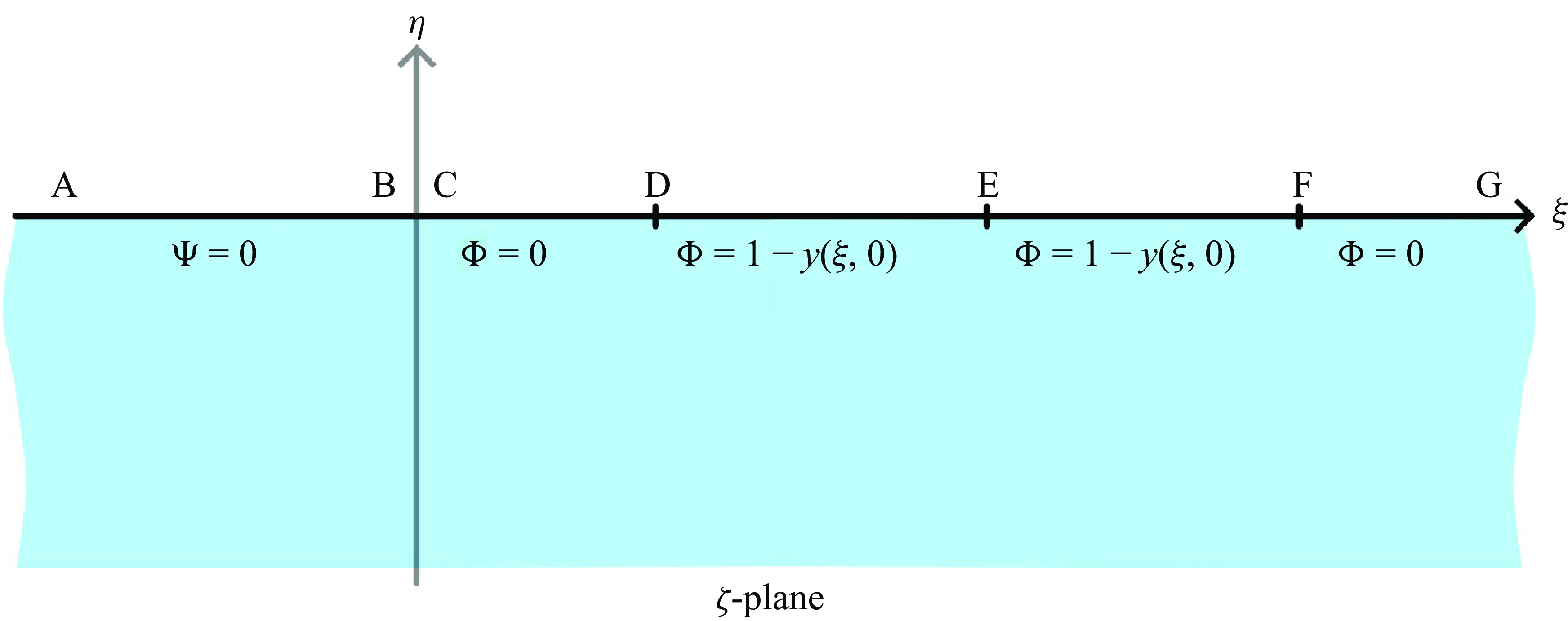
is used. This mapping is known as Schwarz–Christoffel mapping, see chapter 11 in Brown et al. (Reference Brown and Churchill1996), and figure 4 for correspondence of points on the boundaries of the regions in the physical
 $z$
-plane and
 $\zeta $
-plane of the conformal mapping. The mapping
 $z=Z(\zeta )$
has the following behaviour at infinity and zero:
 \begin{align} Z &\sim \frac {1}{\pi }\log \zeta +i+A_{0R},\,\,\texttt{as}\,\,\zeta \to \infty , \end{align}
 \begin{align} Z &\sim \frac {1}{\pi }\log \zeta +i+B_{0R},\,\,\texttt {as}\,\,\zeta \to 0, \\[9pt] \nonumber \end{align}
where
 $A_{0R}$
and
 $B_{0R}$
are real constants. These constants have no effect on the velocity field calculations that are carried out in § 2, § 3 and § 4. The mapping is defined by its derivative
 \begin{eqnarray} \frac {{\rm d}Z}{{\rm d}\zeta }=\frac {1}{\pi \zeta }\left (\frac {(k_1-\zeta )^2}{(k_2-\zeta )(1-\zeta )}\right )^{\alpha /\pi }, \end{eqnarray}
where
 $\alpha =\arctan (1-\delta )$
, and the power term in (3.21) is calculated as
 \begin{align} \left (\frac {(k_1-\zeta )^2}{(k_2-\zeta )(1-\zeta )}\right )^{\alpha /\pi } &= \left (\frac {(-\rho _2e^{i\alpha _2})^2}{(-\rho _3e^{i\alpha _3})(-\rho _1e^{i\alpha _1})}\right )^{\alpha /\pi }\nonumber\\[4pt]&=\left (\frac {\rho _2^2}{\rho _3\rho _1}\right )^{\alpha /\pi } e^{i(2\alpha _2-\alpha _3-\alpha _1)(\alpha /\pi )}. \end{align}
See figure 5 for definitions of
 $\rho _1,\rho _2,\rho _3$
and polar angles
 $\alpha _1, \alpha _2,\alpha _3$
.
The branch cuts and definitions of local polar coordinates.

By integrating (3.21) along the boundary
 $\zeta =\xi -i0$
, we find the relations
 $x(\xi )$
and
 $y(\xi )$
between the coordinates in the
 $\zeta $
-plane and the
 $z$
-plane for the parts of the free surface
 $CD$
,
 $DE$
,
 $EF$
and
 $FG$
, respectively,
 \begin{align} x+iy &=\frac {1}{\pi }\int _1^\xi \frac {1}{\tau }\left (\frac {(\tau -k_1)^2}{(k_2-\tau )(1-\tau )}\right )^{\alpha /\pi }{\rm d} \tau +i-1,\,\,(0\lt \xi \lt 1), \end{align}
 \begin{align} x+iy &=\frac {1}{\pi }e^{-i\alpha }\int _1^\xi \frac {1}{\tau }\left (\frac {(\tau -k_1)^2}{(k_2-\tau )(\tau -1)}\right )^{\alpha /\pi }{\rm d}\tau +i-1,\,\,(1\lt \xi \lt k_1), \end{align}
 \begin{align} x+iy &=\frac {1}{\pi }e^{i\alpha }\int _{k_1}^\xi \frac {1}{\tau }\left (\frac {(\tau -k_1)^2}{(k_2-\tau )(\tau -1)}\right )^{\alpha /\pi }d\tau +i\delta ,\,\,(k_1\lt \xi \lt k_2), \end{align}
 \begin{align} x+iy &=\frac {1}{\pi }\int _{k_2}^\xi \frac {1}{\tau }\left (\frac {(\tau -k_1)^2}{(\tau -k_2)(\tau -1)}\right )^{\alpha /\pi }{\rm d}\tau +i+1,\,\,(\xi \gt k_2). \end{align}
The mapping parameters
 $k_1$
and
 $k_2$
are determined from the asymptotic behaviour of the mapping as
 $\zeta \to 0$
, see (3.20), and the formulae (3.23), (3.25), (3.26). The formula (3.23) gives as
 $\xi \to 0^+$
 \begin{align} x+iy &= \frac {1}{\pi }\left (\frac {k_1^2}{k_2}\right )^{\alpha /\pi }\int _1^\xi \frac {{\rm d}\tau }{\tau }\\ &+\frac {1}{\pi }\int _1^\xi \frac {1}{\tau }\left [\left (\frac {(\tau -k_1)^2}{(k_2-\tau )(1-\tau )}\right )^{\alpha /\pi }-\left (\frac {k_1^2}{k_2}\right )^{\alpha /\pi }\right ]{\rm d}\tau +i-1.\nonumber \end{align}
Comparing the first term in (3.27), which is the leading-order term as
 $\xi \rightarrow 0$
, and (3.20b
) for
 $\zeta =\xi -i0\to 0$
, we conclude
 \begin{eqnarray} k_2=k_1^2. \end{eqnarray}
The formula (3.25) should match (3.26) as
 $\xi \to k_2$
. This condition provides
 \begin{eqnarray} \frac {1}{\pi }e^{i\alpha }\int _{k_1}^{k_2}\frac {1}{\tau }\left (\frac {(\tau -k_1)^2}{(k_2-\tau )(\tau -1)}\right )^{\alpha /\pi }{\rm d}\tau +i\delta =i+1. \end{eqnarray}
By taking the real part of (3.29), we obtain the following:
 \begin{eqnarray} \frac {\pi }{\cos \alpha }=\int _{k_1}^{k_2}\frac {1}{\tau }\left (\frac {(\tau -k_1)^2}{(k_2-\tau )(\tau -1)}\right )^{\alpha /\pi }{\rm d}\tau , \end{eqnarray}
between
 $k_1$
,
 $k_2$
and the angle
 $\alpha$
. Equations (3.28) and (3.30) yield
 $k_1(\alpha )$
. Equation (3.30) is solved by the Newton Raphson method taking (3.28) into account to find numerical values of
 $k_1$
corresponding to fixed
 $\alpha$
values. In figure 6,
 $k_1$
is depicted as a function of
 $\delta$
, where
 $\delta =1-\tan \alpha$
,
 $0\leqslant \delta \leqslant 1$
. It can be shown that
 $k_1(\delta )\to \infty$
as
 $\delta \to 0$
.
The function
 $k_1(\delta )$
.

For
 $\alpha =0$
, (3.21) provides the mapping
 $Z(\zeta )=({1}/{\pi })\log \zeta -i-1$
of the lower half-plane
 $\eta \lt 0$
onto the strip
 $0\lt y\lt 1$
in the
 $z$
-plane. Here
 $\zeta =re^{i\alpha }$
,
 $r\gt 0$
,
 $\pi \lt \alpha \lt 2\pi$
. The correspondence of the points in figure 4 for
 $\delta =1$
,
 $\alpha =0$
gives
 $k_1(1)=e^\pi$
and
 $k_2(1)=e^{2\pi }$
.
3.2. Leading-order velocity potential
The problem (3.1)–(3.8) is reformulated in terms of the complex velocity potential
 $w(\zeta )$
in the lower half-plane
 $\eta \lt 0$
, where
 $w(\zeta )=W(Z(\zeta ))$
,
 $W(Z) = \varphi _0(x,y) + i \psi _0(x,y)$
 \begin{eqnarray} \varphi _0(x,y)+i\psi _0(x,y)=W(z)=W(Z(\zeta ))=w(\zeta )=\varPhi (\xi ,\eta )+i\varPsi (\xi ,\eta ), \end{eqnarray}
where
 $\psi _0(x,y)$
is the leading-order streamfunction.
The flow in the present problem is symmetric with respect to
 $x=0$
. The velocity potential
 $\varphi _0$
at a distance from the cavity,
 $|x|\gt 1$
, is zero on the free surface,
 $y=1$
, and its
 $y$
-derivative is zero at
 $y=0$
. A general form of the velocity potential in
 $|x|\gt 1$
,
 $0\lt y\lt 1$
is
 \begin{align} \varphi _{0}(x,y) &= \mathop\sum\nolimits_{n=0}^{\infty } B_n \cos \left (\frac {\pi }{2}\left ( 2n + 1\right )y\right )e^{-\frac {\pi }{2}(2n+1) |x|}, \end{align}
with certain coefficients
 $B_n$
.
As
 $|x|\rightarrow \infty$
, we have
 $ \varphi _{0}(x,y)\sim B_0 \cos (\pi y /2) e^{-\pi |x| /2}$
, and in another form,
 $ \varphi _{0}(x,y)\sim {Re}[B_0 e^{-\pi z/2}]$
where
 $z=x+iy$
and
 $|x|\rightarrow + \infty$
. The limit
 $|x|\rightarrow + \infty$
corresponds to
 $\zeta \rightarrow \infty$
in the plane of conformal mapping. The asymptotic formula (3.20
a) provides
 $\varPhi (\xi ,\eta )\sim {Re}(1/\sqrt {\zeta })$
as
 $|\zeta |\rightarrow \infty$
. Therefore, the complex velocity potential
 $w(\zeta )$
decays as
 $1/\sqrt {\zeta }$
where
 $|\zeta |\rightarrow \infty$
.
We shall determine the function
 $w(\zeta )$
in the lower half-plane
 $\eta \lt 0$
, which decays as
 $1/\sqrt {\zeta }$
at infinity, and satisfies the following boundary conditions on
 $\eta =0$
:
 \begin{eqnarray} \varPsi (\xi ,0)=0\,\, (\xi \lt 0),\quad &\varPhi (\xi ,0)=0\,\,(0\lt \xi \lt 1\,\, \text{and}\,\, \xi \gt k_2),\nonumber \\ \varPhi (\xi ,0)=1-y(\xi ,0)\,\,&(1\lt \xi \lt k_2), \end{eqnarray}
where
 $y(\xi ,0)$
is given by (3.24), (3.25), see figure 7. Note that
 $1-y(\xi ,0)=(1-\delta )(1-|x(\xi ,0)|)$
where
 $1\lt \xi \lt k_2$
, see (3.3). The boundary conditions (3.33) are of mixed type: the imaginary part of
 $w(\xi -i 0)$
is given on
 $\eta =0$
,
 $\xi \lt 0$
and the real part of
 $w(\xi -i 0)$
is given on
 $\xi \gt 0$
. Such a mixed boundary-value problem can be reduced to a problem for an analytic function, the real part of which is prescribed on the boundary, using the so-called characteristic function
 $R(\zeta )=1/\sqrt {\zeta }$
. This function is defined on the
 $\zeta$
-plane with the cut along the negative
 $\xi$
-axis,
 $\eta =0$
,
 $\xi \lt 0$
. For
 $\zeta =\rho _4 e^{i\alpha _4}$
,
 $\rho _4\gt 0$
,
 $-\pi \lt \alpha _4\lt \pi$
, we have
 $R(\zeta )=\rho _4^{-1/2}e^{-i\alpha _4/2}$
. Then
 $R(\xi )=1/\sqrt {\xi }$
, where
 $\alpha _4=0$
,
 $\xi \gt 0$
,
 $\eta =-0$
and
 $R(\xi )=i/\sqrt {|\xi |}$
, where
 $\alpha _4=-\pi$
,
 $\xi \lt 0$
,
 $\eta =-0.$
The product
 $\tilde {w}(\zeta )=R(\zeta ) w(\zeta )$
is also an analytic function in
 $ \eta \lt 0$
with its real part being given on the boundary
 $\eta =0$
 \begin{align} {Re}(\tilde {w}(\xi -i 0)) = \begin{cases} 0,& \xi \lt 1,\, \xi \gt k_2,\\ \dfrac {1-y(\xi ,0)}{\sqrt {\xi }},& 1\lt \xi \lt k_2. \end{cases} \end{align}
The solution of this boundary problem is given by the Cauchy integral Gakhov (Reference Gakhov1966)
 \begin{eqnarray} \tilde {w}(\zeta )=\frac {i}{\pi }\int _{-\infty }^{\infty } \frac {Re[\tilde {w}(\tau -i0)] {\rm d}\tau }{\tau -\zeta }\quad (\eta \lt 0), \end{eqnarray}
which yields, for the boundary condition (3.34),
 \begin{eqnarray} \tilde {w}(\zeta )=\frac {i}{\pi }\int _{1}^{k_2} \frac {1-y(\tau ,0)}{\sqrt {\tau }(\tau -\zeta )} {\rm d}\tau \quad (\eta \lt 0). \end{eqnarray}
To calculate the flow velocity in the
 $z\hbox{-}$
plane, we differentiate (3.31) and obtain
 \begin{eqnarray} \frac {{\rm d}W}{{\rm d}z}=\frac {{\rm d}w/{\rm d}\zeta }{{\rm d}Z/{\rm d}\zeta }, \end{eqnarray}
where the derivative
 ${\rm d}Z/{\rm d}\zeta$
is given by (3.21) and
 ${\rm d}w/{\rm d}\zeta$
is calculated by differentiating
 $\tilde {w}(\zeta )=R(\zeta )w(\zeta )$
and (3.36).
The leading-order boundary-value problem for the complex potential in the
 $\zeta$
-plane (
 $\eta \lt 0$
).

Dimensionless acceleration of the flow along the rigid bed;
 $\delta =0.5$
.

4. Results and discussion
The leading-order flow accelerations on the boundaries,
 $\textit{AB}$
,
 $\textit{CD}$
,
 $\textit{DE}$
,
 $\textit{EF}$
and
 $\textit{FG}$
, are presented in figures 8 and 9. The flow is symmetric with respect to the
 $y$
-axis. The horizontal and vertical components of the flow acceleration are odd and even functions of
 $x$
, respectively.
Dimensionless horizontal (a) and vertical (b) accelerations of the flow along the free surface for different
 $\delta$
values.

The coefficients of the singular terms of the outer solution,
 $\tilde {C_1}$
and
 $\tilde {C_2}$
, as functions of
 $\delta$
.

The liquid flows towards the cavity along the rigid bed at speed
 $|t\partial \varphi _0/\partial x(x,0)|$
in the leading order. The flow acceleration along the bed is shown in figure 8. It is seen that the maximum acceleration is achieved under the cavity. The dimensionless accelerations,
 $\partial \varphi _0/\partial x$
and
 $\partial \varphi _0/\partial y$
, on the free surface are shown in figure 9. The particles of the free surface move towards the symmetry line horizontally. The particles move downwards at a distance from the symmetry line, which monotonically increases with increase of the parameter
 $\delta$
, and upwards near this line. The leading-order solution derived in § 3.2, is not valid in a close vicinity of the vertex E. This solution should be considered as the outer solution. The problem governing the fine structure of the flow in the small vicinity of point E, as well as the size of this vicinity for small
 $\varepsilon$
, are obtained using methods of asymptotic analysis in § 5. The outer solution and the solution in the vicinity of the vertex E should match one another, in order to make a uniformly valid solution in the leading order as
 $\varepsilon \to 0$
. The outer velocity potential close to the vertex E is given by the asymptotic formula (3.12) which will be used in deriving the leading-order inner solution there. At the other two corner points of the wedge cavity D and F, the linear theory predicts a continuous velocity field but singular derivatives of the velocity, see asymptotic formulae (3.15) and (3.16), and the cusps at these points correspondingly, see (3.19). The solution of § 3.2 should be also corrected in vicinities of points D and F using corresponding inner solutions. The inner solutions should be matched to the outer solution near points D and F, the behaviour of which is described by (3.15). The fine structures of the flows near corners D and F are not studied in this paper.
The products
 $\tilde {C_1}=\gamma C_1$
and
 $\tilde {C_2}=\mu C_2$
, which are the coefficients of the singular parts of the outer velocity of the flow close to the points E and F, correspondingly, are depicted in figure 10 as functions of
 $\delta$
. As
 $\delta \to 1$
, we have
 $\tilde {C_1}\to 1$
and
 $\tilde {C_2}\to 1$
, which corresponds to the limiting case of no motion since the cavity disappears in this limit. At the other limiting case as
 $\delta \to 0$
, where the vertex
 $\textrm{E}$
is on the bottom, we have
 $\tilde {C_2}\to 0.98$
and
 $\tilde {C_1}\to 0$
; this means that the strength of the leading-order flow singularity at the cavity vertex becomes weaker as the vertex approaches the rigid bed. For
 $\delta =0$
, that is when the vertex touches the rigid bed, there is no power-law singularity of the flow velocity at the leading order. The latter case corresponds to the inclined dam-break problem with the dam making a 45-degree angle with the rigid bed. The values of
 $\tilde {C_1}$
and
 $\tilde {C_2}$
in figure 10 are calculated numerically by using a routine of the software package Mathematica 12.0 which is based on the method of general least squares. In this method, the velocity data near the points E and F calculated by the method of § 3.2 are fitted into the curves of the form
 $y=c |x|^{\gamma -1}$
and
 $y=d|x-1|^{\mu -1}$
respectively.
The leading-order free-surface shape is shown in figure 11 for some values of the parameters
 $\delta$
,
 $\varepsilon$
and dimensionless time
 $t$
. The vertical displacement of the free surface is unbounded at the vertex E, see figure 11(a). The predicted free-surface shapes have cusps at the corner points
 $\textrm{D}$
and
 $\textrm{F}$
.
To plot the free-surface shape near F, see figure 11(b), we resort to the Lagrangian variables. The reason for this comes from the definition of the free-surface shapes, see (2.20) and (2.21), where the line
 $x=1$
forms an ‘imaginary’ boundary between the initially horizontal free surface and the initially inclined free surface near F. In this case, it is necessary to let the free-surface fluid particles on either side of the line
 $x=1$
to pass freely to the other side by using the Lagrangian variables. Using (3.15), and the fact that the velocities
 $\bar {u}$
,
 $\bar {v}$
are given as
 \begin{eqnarray} \bar {u}=\frac {{\rm d}\bar {x}}{{\rm d}t}=\varepsilon t \frac {\partial \varphi _0}{\partial \bar {x}},\,\,\bar {v}=\frac {{\rm d}\bar {y}}{{\rm d}t}=\varepsilon t \frac {\partial \varphi _0}{\partial \bar {y}}, \end{eqnarray}
we find the following initial value problem for the position of the fluid particles
 $\bar {x}(t)$
,
 $\bar {y}(t)$
, near the point
 $\textrm{F}$
:
 \begin{align} \frac {{\rm d}\bar {x}}{{\rm d}t}(t)&=\varepsilon \tilde {C_2} t \left (\bar {x}(t)^2+\bar {y}(t)^2\right )^{(\mu -1)/2}\sin \left [(\mu -1)\arctan \left (\frac {\bar {y}(t)}{\bar {x}(t)}\right )\right ],\nonumber \\ \frac {{\rm d}\bar {y}}{{\rm d}t}(t)&=-\varepsilon t+\varepsilon \tilde {C_2} t \left (\bar {x}(t)^2+\bar {y}(t)^2\right )^{(\mu -1)/2}\cos \left [(\mu -1)\arctan \left (\frac {\bar {y}(t)}{\bar {x}(t)}\right )\right ],\nonumber \\ \bar {x}(0)&=\bar {x}_i,\,\,\bar {y}(0)=\bar {y}_i, \end{align}
where
 $(\bar {x}_i,\bar {y}_i)$
,
 $i=1,N$
, are the initial coordinates of the fluid particles on the free surface near
 $\textrm{F}$
, and
 $\tilde {C_2}=1.02$
is used for figure 11.
Dimensionless leading-order free-surface shape;
 $\delta =0.5, \,\varepsilon =0.2, \,t=1$
. (a). Close-up views around the vertices E (b) and F (c).

Problem geometry and meshing in OpenFOAM.

To understand how accurately the theoretical results of § 3.2 describe the evolution of the free surface and the initial flow, the formulated problem of cavity collapse is simulated using the computational fluid dynamics software OpenFOAM. Calculations are performed in the dimensional variables. The numerical domain of the problem is finite and includes both the liquid and air phases. The width of the numerical domain is chosen to be
 $40$
 ${\rm m}$
and the total height is
 $1.2$
 ${\rm m}$
, see figure 12. The initial liquid height outside the cavity is
 $h_2=1$
 ${\rm m}$
and the distance of the wedge vertex E from the bottom is
 $h_1 = 0.5$
 ${\rm m}.$
The domain above the liquid is filled with air. The liquid is incompressible and inviscid with density
 $1000$
 $\rm kg\,m^-{^3}$
. The air is incompressible. The viscosity and density of the air are
 $1.48 \times 10^{-5}$
 $\rm Ns$
and
 $1$
 $\rm kg\,m^-{^3}$
, respectively. Surface tension between the two phases is not included. OpenFOAM uses the volume of fluid method. In this method, the immiscible fluids air and water are considered as one effective fluid throughout the domain. The physical properties of this ‘effective fluid’ are calculated as weighted averages based on the distribution of the liquid volume fraction,
 $\bar {\gamma }$
,
 $0\leqslant \bar {\gamma }\leqslant 1$
. The value
 $\bar {\gamma }=0$
corresponds to the regions containing only air, and
 $\bar {\gamma }=1$
to the regions of pure water. At the interface of water and air,
 $0\lt \bar {\gamma }\lt 1$
. The mathematical model of OpenFOAM consists of the conventional Navier Stokes equations and the supplementary phase fraction equation for capturing the position of the interface between air and water. The boundary conditions are imposed at the sidewalls, the rigid bottom and the atmosphere, see figure 12. On the sidewalls
 $|x'|= 40$
 ${\rm m}$
and the rigid bottom
 $y'=0$
, slip conditions are imposed. For the atmosphere
 $y'=1.2$
 ${\rm m}$
, the total pressure
 $(p+({1}/{2})U^2)$
is initially zero and equal to the internal field value for later times. There is also a velocity condition at the atmosphere, which has zero gradient for outflow and the same value as that of the normal component of the internal cell for inflow. Initially, the fluids are at rest. The meshing, see figure 12, is done in such a way that the cell dimensions are reduced approaching the corner points D, E and F. Reduction of cell size is defined as ‘grading’ in OpenFOAM, which is based on geometric progression. The parameters used in the grading are the expansion ratio, the cell number and the total length. Using these parameters, the minimum cell size is calculated. For the meshing shown in figure 12, the minimum cell size is
 $2.3\, \times \,$
 $2.3$
 ${\rm mm}^2$
. In all OpenFOAM simulations in this paper, the Courant number, which indicates how much the information travels across a computational grid cell in a unit of time, is set to 0.2. It is recommended in the OpenFOAM that for transient flows the Courant number should be less than 1.
Comparisons of the theoretical and numerical velocities on the flow boundaries for
 $\delta = 0.5$
and
 $\varepsilon = 0.1$
at the time instant
 $t'= 0.101 \,\rm s$
are given in figure 13. The agreement is good except in the vicinities of the corner points D, E and F where some discrepancies are expected, since the leading-order outer solution is not valid close to these points. Similarly, for the free-surface shapes, see figure 14, the agreement between the numerical and theoretical results is good except for the corner points. At D and F, the theoretical solution predicts a cusp, whereas the numerical solution predicts a smooth boundary there. At the vertex point E, the boundary displacement is unbounded in the leading-order solution and the numerical method predicts a finite displacement there.
Dimensional horizontal flow velocity on the bottom
 $u'$
(a) and dimensional vertical flow velocity on the free surface
 $v'$
(b) for
 $\delta = 0.5$
,
 $\varepsilon = 0.1$
,
 $t'= 0.101$
 $\rm s$
.

Dimensional leading-order free-surface shape for
 $\delta =0.5, t'=0.143$
(a), and close-up views around the vertices E (b) and F (c).

5. Fine structure of the flow near the vertex of the cavity
Close to the vertex point E of the cavity, the leading-order outer solution derived in § 3.2 predicts a singular flow velocity and infinite displacement of the free surface at the early stage. To find fine details of the flow near the vertex, we zoom a vicinity of the point E introducing stretched inner variables
 \begin{equation} x=\varepsilon ^k \xi , \quad y=\delta +\varepsilon ^k \eta , \end{equation}
where
 $k\gt 0$
and
 $\xi , \eta$
are of
 $\textit {O}(1)$
as
 $\varepsilon \to 0$
. The power
 $k$
is to be determined using the condition that the inner problem is non-trivial and the condition of matching the leading-order inner solution in the variables
 $\xi , \eta , t$
and the outer solution, behaviour of which is described by (3.12) approaching the inner region. Note that
 $\gamma \lt 1$
in (3.12), which yields that the dimensionless velocity potential
 $\varphi (x,y,t)$
as the solution of the problem (2.13)–(2.19) should be sought in the form
 \begin{equation} \varphi (x,y,t) =t(1-\delta )+\varepsilon ^{k\gamma }\varPhi (\xi , \eta , t). \end{equation}
Note that the symmetry of the flow makes it possible to consider only the right side of the inner flow region,
 $\xi \gt 0$
, imposing the condition
 $\varPhi _{\xi }(0,\eta ,t)=0$
on the symmetry line,
 $\xi =0$
. The shape of the free surface provided by the outer solution in the dimensionless variables, see (2.21), (3.4) and (3.12), behaves as
 \begin{equation} y=\delta +(1-\delta )x+ \varepsilon \eta _d(x,t),\quad \eta _d(x,t)\sim \frac {1}{2}(1-\delta )^2 t^2 + \frac {\tilde {C_1}t^2}{2\cos \alpha } x^{\gamma -1}, \end{equation}
close to the vertex point E as
 $x\to 0$
for the right half of the flow domain,
 $x\gt 0$
. The asymptotic formula (5.3) in the inner variables (5.1) reads at the leading order
 \begin{equation} \eta \sim \xi (1-\delta )+\frac {\tilde {C_1}t^2}{2\cos \alpha }\varepsilon ^{k(\gamma -2)+1}\xi ^{\gamma -1}. \end{equation}
The terms on the right-hand side of (5.4) are of the same order as
 $\varepsilon \to 0$
if
 $k=1/(2-\gamma )=(\pi +2\alpha )/(\pi +4\alpha )$
, which defines the dimension of the inner region. The asymptotic formula (5.4) predicts that the shape of the cavity surface in the inner variables should be sought in the form
 \begin{equation} \eta =(1-\delta )\xi +h(\xi ,t) \qquad (\xi \geqslant 0), \end{equation}
where the matching condition of the free-surface shapes in the inner and outer solutions provides
 \begin{equation} h(\xi ,t)\sim \frac {\tilde {C_1}t^2}{2\cos \alpha }\xi ^{\gamma -1}, \end{equation}
as
 $\xi \to +\infty$
. Comparing (5.5) and (2.21), we conclude that
 \begin{equation} \eta _d(x,t)=\varepsilon ^{k-1}h(x/\varepsilon ^k, t). \end{equation}
Correspondingly, the matching condition for the inner velocity potential
 $\varPhi (\xi , \eta , t)$
in the inner polar variables
 $\rho$
and
 $\theta$
, where
 $\xi =\rho \cos \theta$
and
 $\eta =\rho \sin \theta$
, follows from (5.2) and (3.12) and reads
 \begin{equation} \varPhi (\xi , \eta , t)\sim C_1t \rho ^{\gamma }\sin [\gamma (\theta -\alpha )], \end{equation}
where
 $-\pi /2\lt \theta \lt \alpha$
, see (5.5), and
 $\rho \to \infty$
.
Substituting (5.2) and (5.5) in (2.13)–(2.15) and retaining the leading-order terms, we obtain the problem describing the flow close to the vertex point
 \begin{align} {\nabla} ^2\varPhi &=0 \quad (\eta \lt (1-\delta )\xi +h(\xi ,t), \xi \geqslant 0),\nonumber \\ \varPhi _t+\frac {1}{2}|\boldsymbol{\nabla }\varPhi |^2&=0\quad (\eta =(1-\delta )\xi +h(\xi ,t), \xi \geqslant 0),\\ h_t+\varPhi _{\xi }h_{\xi }&=\varPhi _{\eta }-(1-\delta )\varPhi _{\xi }\quad (\eta =(1-\delta )\xi +h(\xi ,t), \xi \geqslant 0),\nonumber \\ \varPhi _{\xi }(0,\eta ,t)&=0\quad (\eta \lt h(0,t))\nonumber . \end{align}
The nonlinear boundary-value problem is supplemented by the conditions at infinity (5.6) and (5.7). The obtained problem does not include the boundary conditions at the bottom of the liquid and on the other parts of the free surface, which are initially horizontal. The leading-order inner problem is independent of gravity, which is the driving force in the original problem. The gravity and other boundaries of the flow region affect the inner flow through the coefficient
 $\tilde {C_1}$
, see figure 10(a), in the far-field conditions.
The solution of the inner problem is self-similar. The self-similar variables can be selected in such a way that the solution in the new variables is independent of time and the coefficient
 $\tilde {C_1}$
, which is responsible for the global geometry of the flow region, and depends only on the angle of the cavity
 $\alpha$
. We are searching for appropriate self-similar variables in the form
 \begin{equation} \hat {\xi }=\frac {\xi }{qt^b},\,\,\hat {\eta }=\frac {\eta }{qt^b},\,\,h(\xi ,t)=qt^b\hat {h}(\hat {\xi }),\,\,\varPhi (\xi ,\eta ,t)=B_1t^a\hat {\varPhi }(\hat {\xi },\hat {\eta }), \end{equation}
where
 $a$
,
 $b$
and
 $q$
are positive numbers. The constants
 $a$
,
 $b$
,
 $q$
and
 $\textrm{B}$
are selected in such a way that (5.6)–(5.9) allow the solution in (5.10) and the boundary-value problem for the new unknown functions
 $\hat {\varPhi }(\hat {\xi },\hat {\eta })$
and
 $\hat {h}(\hat {\xi })$
has the simplest form.
The equation of the free surface in the self-similar variables is
 \begin{equation} \hat {\eta }=(1-\delta )\hat {\xi }+\hat {h}(\hat {\xi }). \end{equation}
The derivatives
 \begin{equation} h_t=bqt^{b-1}(\hat {h}-\hat {\xi }\hat {h}_{\hat {\xi }}),\,\,h_\xi =\hat {h}_{\hat {\xi }}(\hat {\xi }),\,\,\varPhi _\xi =\frac {B_1}{q}t^{a-b}\hat {\varPhi }_{\hat {\xi }}(\hat {\xi },\hat {\eta }),\,\,\varPhi _\eta =\frac {B_1}{q}t^{a-b}\hat {\varPhi }_{\hat {\eta }}(\hat {\xi },\hat {\eta }), \end{equation}
are substituted in the kinematic boundary condition. Then both sides of this condition are divided by
 $bqt^{b-1}$
resulting in
 \begin{equation} \hat {h}-\hat {\xi }\hat {h}_{\hat {\xi }}=\frac {B_1}{bq^2}t^{a+1-2b}\left (\hat {\varPhi }_{\hat {\eta }}-(1-\delta )\hat {\varPhi }_{\hat {\xi }}-\hat {\varPhi }_{\hat {\xi }}\hat {h}_{\hat {\xi }}\right )\,\,\left(\hat {\eta }=(1-\delta )\hat {\xi }+\hat {h}(\hat {\xi }),\,\hat {\xi }=0 \right). \end{equation}
This combination does not include time
 $t$
if
 $2b=a+1$
. To simplify the condition, we require
 $B_1=bq^2$
. The dynamic boundary condition, where
 \begin{equation} \varPhi _t=bB_1t^{a-1}\left (\frac {a}{b}\hat {\varPhi }-\hat {\xi }\hat {\varPhi }_{\hat {\xi }}-\hat {\eta }\hat {\varPhi }_{\hat {\eta }}\right ),\,\,|\boldsymbol{\nabla }\varPhi |^2=\frac {{B_1}^2}{q^2}t^{2a-2b}|\boldsymbol{\nabla }\hat {\varPhi }|^2, \end{equation}
yields using equalities
 $2b=a+1$
and
 $B_1=bq^2$
 \begin{equation} \frac {a}{b}\hat {\varPhi }-\hat {\xi }\hat {\varPhi }_{\hat {\xi }}-\hat {\eta }\hat {\varPhi }_{\hat {\eta }}+\frac {1}{2}|\boldsymbol{\nabla }\hat {\varPhi }|^2=0. \end{equation}
Substituting self-similar variables (5.10) in the far-field conditions (5.6) and (5.7), we find
 \begin{align} \hat {\varPhi }(\hat {\xi },\hat {\eta }) & \sim \frac {C_1q^\gamma }{B_1}t^{1+b\gamma -a}(\hat {\xi }^2+\hat {\eta }^2)^{\gamma /2}\sin [\gamma (\theta -\alpha )], \end{align}
 \begin{align} \hat {h}(\hat {\xi }) &\sim \frac {\gamma C_1 q^{\gamma -2}}{2\cos \alpha }t^{2+b(\gamma -1)-b}\hat {\xi }^{\gamma -1}, \end{align}
as
 $\hat {\xi }\to \infty$
and
 $\hat {\eta }\to \infty$
. Requiring that the right-hand sides in these conditions are independent of time and selecting
 $B_1=C_1q^\gamma$
, we obtain
 \begin{align} a=b\gamma +1,\,\,b &=2+b(\gamma -1),\,\,2b=a+1, \end{align}
 \begin{align} q &=\bigg (\frac {\tilde {C_1}}{b\gamma }\bigg )^{\frac {1}{2-\gamma }},\,\,B_1=bq^2, \end{align}
where
 $\tilde {C_1}(\delta )$
,
 $\delta =1-\tan \alpha$
, is depicted in figure 10(a). Equations (5.18) give
 \begin{equation} b=\frac {2}{2-\gamma },\,\,a=\frac {2+\gamma }{2-\gamma },\,\,\gamma =\frac {\pi }{\pi +2\alpha }. \end{equation}
The boundary-value problem (5.6)–(5.9) in the self-similar variables has the form
 \begin{align} {\nabla} ^2\hat {\varPhi }&=0\,\,\,\big(\hat {\eta }\lt \hat {\xi } \tan \alpha +\hat {h}(\hat {\xi }),\hat {\xi }\gt 0\big),\nonumber \\\frac {2+\gamma }{2}\hat {\varPhi }-\hat {\xi }\hat {\varPhi }_{\hat {\xi }}&-\hat {\eta }\hat {\varPhi }_{\hat {\eta }}+\frac {1}{2}|\boldsymbol{\nabla }\hat {\varPhi }|^2=0\,\,\,\big(\hat {\eta }=\hat {\xi }\tan \alpha +\hat {h}(\hat {\xi }), \hat {\xi }\gt 0\big),\nonumber \\\hat {h}-\hat {\xi }\hat {h}_{\hat {\xi }}=\hat {\varPhi }_{\hat {\eta }}&-\tan \alpha \hat {\varPhi }_{\hat {\xi }}-\hat {\varPhi }_{\hat {\xi }}\hat {h}_{\hat {\xi }}\,\,\,\left(\hat {\eta }=\hat {\xi }\tan \alpha +\hat {h}(\hat {\xi }), \hat {\xi }\gt 0\right),\nonumber \\&\hat {\varPhi }_{\hat {\xi }}(0,\hat {\eta })=0\,\,\,\big(\hat {\eta }\lt \hat {h}(0)\big),\nonumber \\\hat {\varPhi }(\hat {\xi },\hat {\eta }) &\sim \big(\hat {\xi }^2+\hat {\eta }^2\big)^{\gamma /2}\sin \left[\gamma (\theta -\alpha )\right]\,\,\,\left(\hat {\xi }^2+\hat {\eta }^2\to \infty , -\frac {\pi }{2}\lt \theta \lt \alpha \right),\nonumber \\\hat {h}(\hat {\xi }) &\sim \frac {\gamma }{(2-\gamma )\cos \alpha }\hat {\xi }^{\gamma -1}\,\,\,(\hat {\xi }\to \infty ). \end{align}
The problem (5.21) contains only the parameter
 $\alpha$
, which is related to the angle at the cavity vertex. The potential
 $\hat {\varPhi }(\hat {\xi },\hat {\eta })$
increases in the far field as
 $\hat {\xi }^2+\hat {\eta }^2\to \infty$
. However, on the free surface,
 $\hat {\eta }=\hat {\xi }\tan \alpha +\hat {h}(\hat {\xi })$
,
 $\hat {\xi }\to \infty$
, it decays as
 $O(\hat {\xi }^{\gamma -2})$
because
 $\theta \to \alpha$
there. The problem (5.21) is similar to the inner self-similar problems considered in Iafrati et al. (Reference Iafrati and Korobkin2004), Martinez-Legazpi et al. (Reference Martìnez-Legazpi, Korobkin and Lasheras2015) and Iafrati (Reference Iafrati2012).
Using a new unknown function
 $S(\hat {\xi },\hat {\eta })=({1}/{2})(\hat {\xi }^2+\hat {\eta }^2)-\hat {\varPhi }(\hat {\xi },\hat {\eta })$
, the boundary conditions of problem (5.21) can be simplified. The kinematic boundary condition gives that the normal derivative
 $\partial S/\partial n=0$
on the free surface, and the dynamic boundary condition provides
 $S_{\tau }^{2}=(2+\gamma )S-({1}/{2})\gamma (\hat {\xi }^2+\hat {\eta }^2)$
on the free surface, where
 $S_\tau$
is the tangential derivative. The latter condition can be integrated along the free surface, if the shape of the free surface is known. This technique was used in Iafrati et al. (Reference Iafrati and Korobkin2004) and Iafrati (Reference Iafrati2012) to find higher-order terms in the far-field asymptotics of the solutions to the corresponding self-similar problems. The problem (5.21) can be solved numerically by the boundary element method. The function
 $S(\xi ,\eta )$
helps us to find the higher-order terms in the far-field asymptotic behaviour of the solution, which significantly reduces the numerical domain. See Iafrati et al. (Reference Iafrati and Korobkin2004), Iafrati (Reference Iafrati2012) and Martinez-Legazpi et al. (Reference Martìnez-Legazpi, Korobkin and Lasheras2015) for details. Figure 15 shows the time evolution of the free-surface shape near the vertex E by OpenFOAM with two different meshings, which confirms that the flow is mesh-independent. Also, we observe that the results near vertex are self-similar. This shows that both meshings predict a similar shape for the complicated jet head. It is highly probable that the boundary element solution of the inner region problem will reveal more details of the jet head, which was indeed the case in Martinez-Legazpi et al. (Reference Martìnez-Legazpi, Korobkin and Lasheras2015).
Time evolution of the free surface near the vertex E for
 $0\lt t'\lt 0.14$
s and
 $\delta =0.5$
by OpenFOAM with two different meshings: black lines are obtained using the meshing with minimum cell size of
 $2.3$
 $\times$
 $2.3$
 $\rm mm^2$
and red lines with minimum cell size of
 $1.23$
 $\times$
 $1.23$
 $\rm mm^2$
.

6. Conclusions
Short-time behaviour of two-dimensional gravity-driven flow of a fluid that initially has a wedge-shaped cavity at the free surface is examined analytically and numerically. The maximum leading-order flow acceleration along the rigid bed is achieved at some point under the cavity. At the free surface the fluid particles move towards the symmetry line horizontally and they move downwards at some distance from the symmetry line and upwards near this line.
It is shown by local analysis that the leading-order flow velocity exhibits a power-law singularity at the vertex of the wedge and that the power of the singularity depends on the wedge angle. As the initial wedge cavity becomes bigger and extends towards the rigid basin, the finite-depth effects become more important, and the leading-order flow singularity at the vertex becomes stronger. The similarities between the present problem and the wet-bed dam-break problem are established, namely that the flow velocities in both problems exhibit power-law singularities near the corner points. At the other two corner points, D and F, the flow velocity is continuous but the velocity gradient is not.
The theoretical results are compared with the numerical ones by OpenFOAM, and the agreement is generally good except for the vicinities of the vertex point E where the linear theory fails and the corner points D and F where the linear theory predicts a corner in the free-surface shape. At the vertex point E, the boundary displacement is unbounded in the leading order and the numerical method predicts a finite displacement there. At the other two corner points of the wedge, D and F, while the linear theory predicts a continuous velocity field but discontinuous velocity gradient field of the flow, the numerical results predict a smooth flow.
The leading-order solution is clearly not valid near the vertex. Inner region formulations are derived near the vertex point of the wedge, which shows that the local flow near the vertex is self-similar. The OpenFOAM simulations confirm that the flow near the vertex is indeed self-similar and that the jet head has a complicated shape.
Local problem around the corner point
 $E(0,\delta)$

For a future work, three-dimensional effects are to be investigated by replacing the two-dimensional wedge by a circular or elliptical cone.
Acknowledgements
The authors are grateful to the referees for their important comments, which helped improve the paper.
Declaration of interests
The authors report no conflict of interest.
Appendix A.
In polar coordinates
 $(\tilde {r},\tilde {\theta })$
near the corner point
 $\textrm{E}$
, the Laplace equation and the associated boundary conditions can be expressed as shown in figure 16
 \begin{align} \frac {\partial ^2 \varphi _0}{\partial \tilde {r}^2} + \frac {1}{\tilde {r}} \frac {\partial \varphi _0}{\partial \tilde {r}} + \frac {1}{\tilde {r}^2} \frac {\partial ^2 \varphi _0}{\partial \tilde {\theta }^2} &= 0, \end{align}
 \begin{align} \varphi _0(\tilde {x},\tilde {y})=1-\delta -\tilde {y}=(1-\delta )(1-|\tilde {x}|)\,\, \text{on}\,\,\tilde {\theta }&=\alpha \, \text{and}\,\,\tilde {\theta }=-\pi -\alpha . \end{align}
We seek the solution of the form
 \begin{eqnarray} \varphi _0(\tilde {r}, \tilde {\theta }) = 1-(\delta +\tilde {y}) + \varphi _{00}(\tilde {r}, \tilde {\theta }), \end{eqnarray}
where
 $ \varphi _{00}$
satisfies the Laplace equation and homogeneous boundary conditions
 \begin{eqnarray} {\nabla} ^2 \varphi _{00}=0,\ \varphi _{00}\big |_{\tilde {\theta }=\alpha }=0\ \text{and} \ \varphi _{00}\big |_{\tilde {\theta }=-\pi -\alpha }=0. \end{eqnarray}
We obtain the solution
 $\varphi _{00}$
by using separation of variables in the form,
 $\varphi _{00}=R(\tilde {r})\varTheta (\tilde {\theta })$
. The regular solution at the origin takes the form
 $R(\tilde {r}) = \tilde {r}^{\gamma }$
while the angular part is given by
 $\varTheta (\tilde {\theta }) = C_1\sin (\gamma \tilde {\theta }) + C_2\cos (\gamma \tilde {\theta })$
. Considering the homogeneous boundary conditions, we find
 $\gamma _n= \pi n/ (\pi +2\alpha )$
,
 $n \in \mathbb{Z}$
. Since
 $\varphi _{00}$
is bounded for
 $n \geqslant 1$
, we can write the general solution as follows:
 \begin{eqnarray} \varphi _{00}=\sum _{n=1}^\infty C_n \tilde {r}^\gamma \sin \big(\gamma _n(\tilde {\theta }-\alpha )\big). \end{eqnarray}
Thus, the corresponding leading-order eigenvalue solution given in (A3) for the local problem defined in (A1) can be expressed as follows:
 \begin{align} \varphi _0(\tilde {x},\tilde {y})=(1-\delta -\tilde {y})+C_1\tilde {r}^{\gamma }\sin \big [\gamma (\tilde {\theta }-\alpha )\big ]+o(\tilde {r}^\gamma ). \end{align}
Appendix B.
To analyse the solution near the corner point F, we consider the Laplace equation in the polar coordinates
 $(\bar {r},\bar {\theta })$
as illustrated in figure 17. The Laplace equation is accompanied by the following boundary conditions:
 \begin{eqnarray} \varphi _0(\overline {r},0)=0, \quad \varphi _0(\overline {r},-\pi +\alpha )=-\bar {y}=-(1-\delta )\bar {x}. \end{eqnarray}
We propose a decomposition of the velocity potential of the form
 \begin{eqnarray} \varphi _0(\overline {r},\overline {\theta })=-\overline {r}\sin {\overline {\theta }}+ \varphi _{00}(\overline {r},\overline {\theta }) \end{eqnarray}
where the term
 $ \varphi _{00}$
satisfies a homogeneous Laplace problem
 \begin{eqnarray} {\nabla} ^2 \varphi _{00}=0,\ \varphi _{00}\big |_{\bar {\theta }=0}=0\ \text{and} \ \varphi _{00}\big |_{\bar {\theta }=-\pi +\alpha }=0. \end{eqnarray}
By applying the method of separation of variables, we express the solution as
 $\varphi _{00} = R(\bar {r})\varTheta (\bar {\theta })$
with
 $ R(\bar {r})=\bar {r}^\mu$
and
 $\varTheta (\bar {\theta }) = C_2\sin (\mu \bar {\theta }) + C_3\cos (\mu \bar {\theta })$
.
Imposing the homogenous boundary conditions in (B3), we find
 $\mu _n=\pi n /(\alpha -\pi )$
,
 $n \in \mathbb{Z}$
. The general bounded solution is therefore given by
 \begin{eqnarray} \varphi _{00}(\bar {r},\bar {\theta })=\sum _{n=1}^\infty C_{n+1} \bar {r}^\mu \sin (\mu _n(\bar {\theta }-\alpha )). \end{eqnarray}
It follows that the leading-order solution of the local problem (B1) as
 $\bar {r}\rightarrow 0$
behaves as
 \begin{align} \varphi _0(\bar {r},\bar {\theta })=-\overline {r}\sin {\overline {\theta }}+C_2\overline {r}^{\mu }\sin \left (\mu \overline {\theta }\right )+O(\bar {r}^{2\mu }). \end{align}
This potential satisfies the Laplace equation in the sector
 $-\pi +\alpha \lt \bar {\theta }\lt 0$
and the boundary conditions
 $\varphi _0(\overline {r},0)=0$
,
 $\varphi _0(\overline {r},-\pi +\alpha )=-(1-\delta )\bar {x}$
, where
 $\mu =\pi /(\pi -\alpha )$
,
 $1\lt \mu \lt 4/3$
. We use here that
 $1-\delta =\tan \alpha$
and
 $(1-\delta )\bar {x}=(1-\delta )\bar {r}\text{cos}(-\pi +\alpha )=\bar {r}\tan \alpha \cos (-\pi +\alpha )=\bar {r}\sin (-\pi +\alpha )$
at
 $\bar {\theta }=-\pi +\alpha$
.
Local problem around the corner point
 $F(1,1)$
.