1 Introduction
Major developments have been made to Boussinesq-type (BT) models of water waves over the last five decades following the works of Peregrine (Reference Peregrine1967), Madsen, Murray & Sörensen (Reference Madsen, Murray and Sörensen1991) and Nwogu (Reference Nwogu1993). An attractive attribute of a conventional BT model is that it is able to reduce a complex three-dimensional (3D) problem into a two-dimensional (2D) problem, thereby greatly reducing the computational cost. Therefore, many numerical codes employing BT models have been developed to simulate water wave propagation, including the Mike21 commercial software tool (BT models) and the open-source codes FUNWAVE and COULWAVE. Antuono, Liapidevskii & Brocchini (Reference Antuono, Liapidevskii and Brocchini2009) proposed a novel approach to extending the nonlinear shallow-water equations with dispersive terms to form a hyperbolic BT model. The resulting equations can model nearshore dynamics and offer a complete representation of dispersive and nonlinear wave phenomena. The hyperbolic BT model is computationally efficient and overcomes many limitations of conventional BT models. Comprehensive reviews on BT model theories can be found in Madsen & Fuhrman (Reference Madsen, Fuhrman and Ma2010), Brocchini (Reference Brocchini2013) and Kirby (Reference Kirby2016).
Dispersion is among the most crucial properties of BT models. An accurate representation of dispersion is crucial for simulating surface waves in deep water, and many BT models have been developed to achieve such a goal. An accurate prediction of wave motions in a BT model requires accurate representations of other properties as well, including velocity profiles, shoaling amplitude and nonlinear wave–wave interaction to match the accuracy of dispersion. Unfortunately, most of the existing models are unable to ensure accurate representations of all those quantities due to the different approximations employed in these models. For example, fourth-order BT models are considered as the most accurate models in the framework of conventional Boussinesq equations. Because these fourth-order BT models usually employ a Padé
 $[4,4]$
approximation to the exact wave celerity, their applications are limited by the deep-water limit (
 $kh=6.0$
), and the limit is further reduced with respect to nonlinearity. The third-order transfer function and amplitude dispersion in the fourth-order BT models by Madsen & Schäffer (Reference Madsen and Schäffer1998) and Zou & Fang (Reference Zou and Fang2008) can achieve reasonable accuracies only for
 $kh<0.5$
, and the corresponding second-order transfer function achieves a slightly better accuracy range that extends to
 $kh=1.0$
. The other available fourth-order BT model developed by Gobbi & Kirby (Reference Gobbi and Kirby2000) exhibits some relatively accurate second-order superharmonics up to
 $kh=3.0$
, and second-order subharmonics are accurate only for water depths of up to
 $kh=1.2$
. Thus, improvements can be made to extend the water depth limits for BT models.
Among the various properties embodied in BT models, high dispersion and nonlinearity are the most promising attributes that can lead to high accuracy (e.g. Agnon, Madsen & Schäffer Reference Agnon, Madsen and Schäffer1999; Madsen, Bingham & Liu Reference Madsen, Bingham and Liu2002; Madsen, Bingham & Schäffer Reference Madsen, Bingham and Schäffer2003; Madsen, Fuhrman & Wang Reference Madsen, Fuhrman and Wang2006; Chazel et al. Reference Chazel, Benoit, Ern and Piperno2009; Antuono & Brocchini Reference Antuono and Brocchini2013; Liu & Fang Reference Liu and Fang2016). Like their unique characteristics, the vertical velocity component in highly dispersive and nonlinear BT models is retained in the governing equations, whereas the vertical velocity in conventional BT models is expressed as a function of horizontal velocity, and its explicit appearance is excluded from the governing equations. Two approaches are usually employed to derive highly dispersive and nonlinear BT models.
The first approach was introduced by Agnon et al. (Reference Agnon, Madsen and Schäffer1999) based on an exact formulation of the boundary conditions at the free surface and sea bottom combined with an approximate solution to the Laplace equation that is expressed in terms of a truncated series expansion. The model consists of six coupled equations for surface elevation, horizontal gradient of the velocity potential at the surface, horizontal and vertical velocity components at the surface, and still water level. The approach was further generalized by Madsen et al. (Reference Madsen, Bingham and Liu2002) to obtain accurate velocity profiles in two main steps. The first step involves generalizing the velocities at the still water level by using the velocities defined at an arbitrary water depth, and the second step involves replacing the velocities at the arbitrary water depth by one computational horizontal velocity vector and one vertical velocity to achieve the Padé approximation that is valid at both the still water level and the bottom location.
The second approach is the multi-layer concept proposed by Lynett & Liu (Reference Lynett and Liu2004a ,Reference Lynett and Liu b ), who used several separate quadratic velocity polynomials that are matched at the interfaces between adjacent layers to avoid calculating fifth-order derivatives in BT models. Thus only the third-order spatial derivatives remain in the governing equations, which is especially convenient for coding.
Chazel et al. (Reference Chazel, Benoit, Ern and Piperno2009) and Liu & Fang (Reference Liu and Fang2016) developed a two-layer BT model for highly dispersive and nonlinear waves by combining the two aforementioned approaches. Chazel et al. (Reference Chazel, Benoit, Ern and Piperno2009) derived a double-layer BT model that is expressed by two pseudo-horizontal velocity potentials and two pseudo-vertical velocities, where the highest spatial derivative is second-order, and they reported excellent linear and nonlinear properties of that model. Liu & Fang (Reference Liu and Fang2016) reviewed the findings of previous studies (Madsen et al.
Reference Madsen, Bingham and Liu2002, Reference Madsen, Fuhrman and Wang2006; Lynett & Liu Reference Lynett and Liu2004b
; Liu & Fang Reference Liu and Fang2015) and formulated a BT model according to two groups of horizontal and vertical velocities that are defined at mid-depth in each layer before replacing those velocities with the computational horizontal and vertical velocities to obtain the Padé approximation at the still water level, interface and sea bottom, where the highest spatial derivative is third-order. This new BT model is applicable up to
 $kh\approx 53$
in linear dispersion, up to
 $kh\approx 30$
in the second-order nonlinear property (with a 1 % error) and up to
 $0<kh<60$
in the linear shoaling property (with a 0.13 % error). Antuono & Brocchini (Reference Antuono and Brocchini2013) proposed another interesting approach starting from the Reynolds equations, and they decomposed the velocity into depth-averaged components and deviations from the mean profiles and obtained an integro-differential Boussinesq model with accurate linear dispersion for monochromatic waves.
In this paper, the two-layer model reported by Liu & Fang (Reference Liu and Fang2016) is extended to a new multi-layer irrotational BT model. The proposed multi-layer model achieves the following improvements over the two-layer model reported by Liu & Fang (Reference Liu and Fang2016). (1) Although Liu & Fang (Reference Liu and Fang2016) achieved high accuracy by combining the two classical approaches, the potential of their model in extremely deep waters has not been fully demonstrated. The present study presents a complete model through vigorous derivations and analysis and demonstrates the efficiency of the model through comparisons with analytical solutions and experimental results. (2) A reduced order of the new multi-layer BT model with second-order spatial derivatives and an enhanced order model with fifth-order spatial derivatives (see details in the main text) are proposed to broaden the applications of the new model. (3) A numerical implementation of the new model is conducted to validate the proposed model. To the best of the authors’ knowledge, this is the second study of a multi-layer BT model following that of Lynett & Liu (Reference Lynett and Liu2004a ). The derivations and theoretical analysis offered in this study provide further insights into the multi-layer BT model.
The remainder of this paper is organized as follows. Section 2 describes the systematic derivation of the multi-layer BT model. Section 3 presents an analysis of the linear properties of the model, including wave celerity, linear velocity profile, linear shoaling gradient, shoaling amplitude and their nonlinear properties, including the second-order nonlinear harmonics for regular waves and the sub- and superharmonics for bichromatic waves, third-order harmonics and amplitude dispersion. Section 4 introduces two versions of multi-layer BT models for which the highest derivatives are second-order and fifth-order. Section 5 presents a numerical solution of the vertical 2D form of the four-layer BT equations and numerical results to validate the model. Section 6 provides the conclusions.
2 Derivation of the Boussinesq-type equations
The Cartesian coordinate system is used, where the
 $x$
- and
 $y$
-axes are located on the mean water surface and the
 $z$
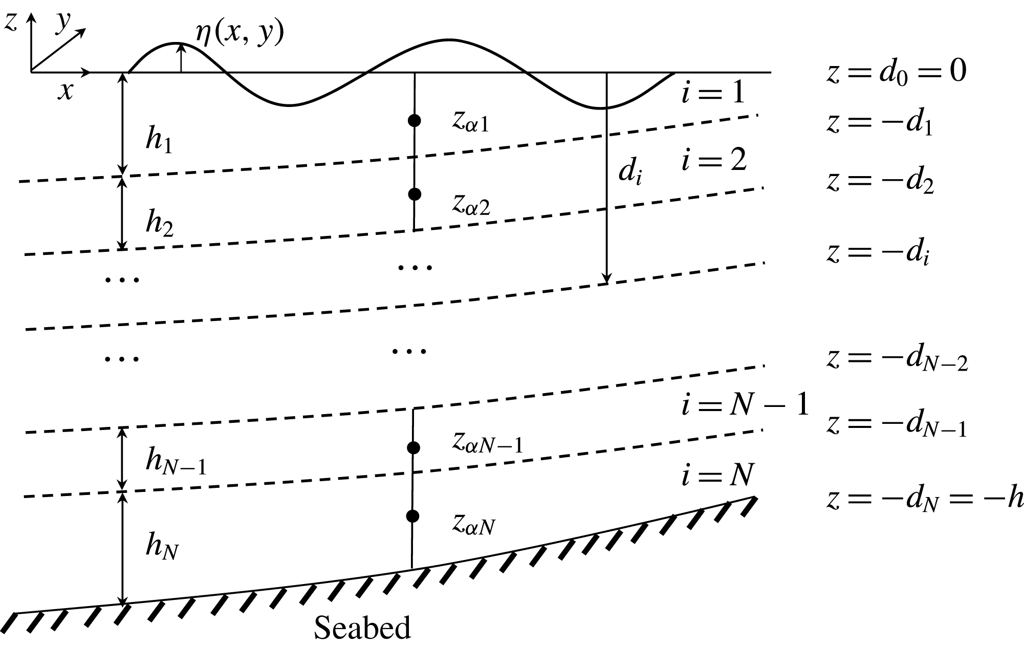
-axis points vertically upwards, as shown in figure 1. In this figure,
 $\unicode[STIX]{x1D702}(x,y,t)$
is the surface elevation measured from the mean water level,
 $z=0$
,
 $h_{i}(x,y)$
is the thickness of the
 $i$
th layer, and
 $z_{\unicode[STIX]{x1D6FC}i}$
represents the location where the velocity components are defined in the
 $i$
th layer (e.g.
 $\unicode[STIX]{x1D6FC}_{i}=0.5$
, which corresponds to the mid-layer location). The interface location between adjacent layers
 $d_{i}$
is defined as follows (measured from the still water level):
 $$\begin{eqnarray}\displaystyle d_{i}=\mathop{\sum }_{j=1}^{i}h_{j}, & & \displaystyle\end{eqnarray}$$
with
 $d_{0}=0$
in the following derivations.
Schematic of a multi-layer concept for waves propagating over a slowly varying seabed. The dashed lines represent the locations of the interfaces between adjacent layers.

2.1 Governing equations
Assuming that the fluid is irrotational, a velocity potential
 $\unicode[STIX]{x1D753}$
exists in the interior fluid domain bounded by the seabed
 $z=-h(x,y)$
and the free surface
 $z=\unicode[STIX]{x1D702}(x,y,t)$
. To facilitate the utilization of the multi-layer approach, the potential
 $\unicode[STIX]{x1D753}$
is decomposed into
 $N$
groups (i.e.
 $\unicode[STIX]{x1D753}_{i}(x,y,z,t),~i=1,2,\ldots ,N$
) in the following derivation. These velocity potentials are governed by the following Laplace equation:
 $$\begin{eqnarray}\displaystyle \unicode[STIX]{x1D6FB}^{2}\unicode[STIX]{x1D753}_{i}+\unicode[STIX]{x1D753}_{izz}=0,\quad i=1,2,\ldots ,N, & & \displaystyle\end{eqnarray}$$
where subscript
 $z$
represents the partial derivative with respect to
 $z$
.
The Laplace equation (2.2) together with the irrotational assumption can be written as follows:
 $$\begin{eqnarray}\displaystyle (\unicode[STIX]{x1D735}\boldsymbol{\cdot }\boldsymbol{u}+w_{z})_{i}=0,\quad (\unicode[STIX]{x1D735}w-\boldsymbol{u}_{z})_{i}=0, & & \displaystyle\end{eqnarray}$$
where
 $\boldsymbol{u}_{i}=\unicode[STIX]{x1D735}\unicode[STIX]{x1D753}_{i},~w_{i}=\unicode[STIX]{x1D753}_{iz}$
.
The kinematic and dynamic boundary conditions on the free surface are written as
 $$\begin{eqnarray}\displaystyle \unicode[STIX]{x1D702}_{t}+\unicode[STIX]{x1D735}\unicode[STIX]{x1D753}\boldsymbol{\cdot }\unicode[STIX]{x1D735}\unicode[STIX]{x1D702}=\unicode[STIX]{x1D753}_{z} & & \displaystyle\end{eqnarray}$$
and
 $$\begin{eqnarray}\displaystyle (\unicode[STIX]{x1D753}_{t}+\unicode[STIX]{x1D702})+{\textstyle \frac{1}{2}}[(\unicode[STIX]{x1D735}\unicode[STIX]{x1D753})^{2}+\unicode[STIX]{x1D753}_{z}^{2}]=0. & & \displaystyle\end{eqnarray}$$
According to previous studies (Agnon et al. Reference Agnon, Madsen and Schäffer1999; Madsen et al. Reference Madsen, Bingham and Liu2002; Liu & Fang Reference Liu and Fang2016), equations (2.4) and (2.5) can be expressed as follows according to the velocities defined on the free surface:
 $$\begin{eqnarray}\displaystyle & \displaystyle \unicode[STIX]{x1D702}_{t}+\boldsymbol{U}\boldsymbol{\cdot }\unicode[STIX]{x1D735}\unicode[STIX]{x1D702}-w_{\unicode[STIX]{x1D702}}(1+\unicode[STIX]{x1D735}\unicode[STIX]{x1D702}\boldsymbol{\cdot }\unicode[STIX]{x1D735}\unicode[STIX]{x1D702})=0, & \displaystyle\end{eqnarray}$$
 $$\begin{eqnarray}\displaystyle & \displaystyle \boldsymbol{U}_{t}+g\unicode[STIX]{x1D735}\unicode[STIX]{x1D702}+{\textstyle \frac{1}{2}}\unicode[STIX]{x1D735}[\boldsymbol{U}\boldsymbol{\cdot }\boldsymbol{U}-w_{\unicode[STIX]{x1D702}}^{2}(1+\unicode[STIX]{x1D735}\unicode[STIX]{x1D702}\boldsymbol{\cdot }\unicode[STIX]{x1D735}\unicode[STIX]{x1D702})]=0 & \displaystyle\end{eqnarray}$$
and
 $$\begin{eqnarray}\displaystyle \boldsymbol{U}=\boldsymbol{u}_{\unicode[STIX]{x1D702}}+w_{\unicode[STIX]{x1D702}}\unicode[STIX]{x1D735}\unicode[STIX]{x1D702}, & & \displaystyle\end{eqnarray}$$
where
 $\boldsymbol{U}$
is the horizontal gradient of the velocity potential defined on the free surface,
 $\boldsymbol{u}_{\unicode[STIX]{x1D702}}$
and
 $w_{\unicode[STIX]{x1D702}}$
are the horizontal velocity vector and the vertical velocity component defined on the free surface, respectively, and
 $g$
is the acceleration due to gravity.
The kinematic boundary condition at the sea bottom is expressed as
 $$\begin{eqnarray}\displaystyle \boldsymbol{u}\boldsymbol{\cdot }\unicode[STIX]{x1D735}h+w=0,\quad z=-h. & & \displaystyle\end{eqnarray}$$
The following matching conditions are used to establish a relationship between the velocities at the interface of two adjacent layers:
 $$\begin{eqnarray}\displaystyle \boldsymbol{u}_{i}(x,-d_{i},t)=\boldsymbol{u}_{i+1}(x,-d_{i},t),\quad w_{i}(x,-d_{i},t)=w_{i+1}(x,-d_{i},t). & & \displaystyle\end{eqnarray}$$
2.2 Velocity field expressed in terms of the velocities defined at the mid-water depth using the Taylor expansion method
Following Liu & Fang (Reference Liu and Fang2016), the actual velocity components are defined at the mid-depth location of each layer (see figure 1). The horizontal velocity vector and vertical velocity component in each layer are defined as
 $\boldsymbol{u}_{\unicode[STIX]{x1D6FC}i}=\boldsymbol{u}(\boldsymbol{x},z_{\unicode[STIX]{x1D6FC}i}(\boldsymbol{x}),t)$
and
 $w_{\unicode[STIX]{x1D6FC}i}=w(\boldsymbol{x},z_{\unicode[STIX]{x1D6FC}i}(\boldsymbol{x}),t)$
, respectively. Based on the
 $N$
groups of velocities, equation (2.3) can be reformulated as
 $$\begin{eqnarray}\displaystyle \unicode[STIX]{x1D735}\boldsymbol{\cdot }\boldsymbol{u}_{\unicode[STIX]{x1D6FC}i}-\unicode[STIX]{x1D735}z_{\unicode[STIX]{x1D6FC}i}\boldsymbol{\cdot }\boldsymbol{u}_{\unicode[STIX]{x1D6FC}iz}+w_{\unicode[STIX]{x1D6FC}iz}=0,\quad \unicode[STIX]{x1D735}w_{\unicode[STIX]{x1D6FC}i}-\unicode[STIX]{x1D735}z_{\unicode[STIX]{x1D6FC}i}w_{\unicode[STIX]{x1D6FC}iz}-\boldsymbol{u}_{\unicode[STIX]{x1D6FC}iz}=0, & & \displaystyle\end{eqnarray}$$
where
 $\unicode[STIX]{x1D735}\boldsymbol{\cdot }\boldsymbol{u}_{\unicode[STIX]{x1D6FC}i}=\unicode[STIX]{x1D735}\boldsymbol{\cdot }(\boldsymbol{u}|_{z=z_{\unicode[STIX]{x1D6FC}i}}),~\boldsymbol{u}_{\unicode[STIX]{x1D6FC}iz}=\unicode[STIX]{x2202}\boldsymbol{u}/\unicode[STIX]{x2202}z|_{z=z_{\unicode[STIX]{x1D6FC}i}},~\unicode[STIX]{x1D735}w_{\unicode[STIX]{x1D6FC}i}=\unicode[STIX]{x1D735}(w|_{z=z_{\unicode[STIX]{x1D6FC}i}}),~w_{\unicode[STIX]{x1D6FC}iz}=\unicode[STIX]{x2202}w/\unicode[STIX]{x2202}z|_{z=z_{\unicode[STIX]{x1D6FC}i}}$
,
 $z_{\unicode[STIX]{x1D6FC}1}=-(1/2)h_{1}$
and
 $z_{\unicode[STIX]{x1D6FC}(i+1)}=z_{\unicode[STIX]{x1D6FC}i}-(1/2)(h_{i}+h_{i+1})$
.
The high-order terms related to
 $(\unicode[STIX]{x1D735}z_{\unicode[STIX]{x1D6FC}})^{2}$
and
 $\unicode[STIX]{x1D6FB}^{2}z_{\unicode[STIX]{x1D6FC}}$
represent the effects of the high-order derivatives and are valid only for
 $kh<6$
(Madsen et al.
Reference Madsen, Fuhrman and Wang2006). Thus, without loss of generality, these high-order terms are neglected for brevity. Therefore, the present model is derived under a mild slope assumption. From (2.11), we obtain the following:
 $$\begin{eqnarray}\displaystyle w_{\unicode[STIX]{x1D6FC}iz}=-\unicode[STIX]{x1D735}\boldsymbol{\cdot }\boldsymbol{u}_{\unicode[STIX]{x1D6FC}i}+\unicode[STIX]{x1D735}z_{\unicode[STIX]{x1D6FC}i}\boldsymbol{\cdot }\unicode[STIX]{x1D735}w_{\unicode[STIX]{x1D6FC}i},\quad \boldsymbol{u}_{\unicode[STIX]{x1D6FC}iz}=\unicode[STIX]{x1D735}w_{\unicode[STIX]{x1D6FC}i}+\unicode[STIX]{x1D735}z_{\unicode[STIX]{x1D6FC}i}\unicode[STIX]{x1D735}\boldsymbol{\cdot }\boldsymbol{u}_{\unicode[STIX]{x1D6FC}i}, & & \displaystyle\end{eqnarray}$$
 $$\begin{eqnarray}\displaystyle w_{\unicode[STIX]{x1D6FC}izz}=-\unicode[STIX]{x1D6FB}^{2}w_{\unicode[STIX]{x1D6FC}i}-2\unicode[STIX]{x1D735}z_{\unicode[STIX]{x1D6FC}i}\boldsymbol{\cdot }\unicode[STIX]{x1D6FB}^{2}\boldsymbol{u}_{\unicode[STIX]{x1D6FC}i},\quad \boldsymbol{u}_{\unicode[STIX]{x1D6FC}izz}=-\unicode[STIX]{x1D6FB}^{2}\boldsymbol{u}_{\unicode[STIX]{x1D6FC}i}+2\unicode[STIX]{x1D735}z_{\unicode[STIX]{x1D6FC}i}\unicode[STIX]{x1D6FB}^{2}w_{\unicode[STIX]{x1D6FC}i} & & \displaystyle\end{eqnarray}$$
and
 $$\begin{eqnarray}\displaystyle w_{\unicode[STIX]{x1D6FC}izzz}=\unicode[STIX]{x1D6FB}^{3}\boldsymbol{u}_{\unicode[STIX]{x1D6FC}i}-3\unicode[STIX]{x1D735}z_{\unicode[STIX]{x1D6FC}i}\boldsymbol{\cdot }\unicode[STIX]{x1D6FB}^{3}w_{\unicode[STIX]{x1D6FC}i},\quad \boldsymbol{u}_{\unicode[STIX]{x1D6FC}izzz}=-\unicode[STIX]{x1D6FB}^{3}w_{\unicode[STIX]{x1D6FC}i}-3\unicode[STIX]{x1D735}z_{\unicode[STIX]{x1D6FC}i}\unicode[STIX]{x1D6FB}^{3}\boldsymbol{u}_{\unicode[STIX]{x1D6FC}i}, & & \displaystyle\end{eqnarray}$$
where
 $$\begin{eqnarray}\displaystyle \unicode[STIX]{x1D6FB}^{2}\boldsymbol{u}_{\unicode[STIX]{x1D6FC}i}=\unicode[STIX]{x1D735}(\unicode[STIX]{x1D735}\boldsymbol{\cdot }\boldsymbol{u}_{\unicode[STIX]{x1D6FC}i}),\quad \!\unicode[STIX]{x1D6FB}^{3}\boldsymbol{u}_{\unicode[STIX]{x1D6FC}i}=\unicode[STIX]{x1D735}\boldsymbol{\cdot }(\unicode[STIX]{x1D6FB}^{2}\boldsymbol{u}_{\unicode[STIX]{x1D6FC}i}),\quad \!\unicode[STIX]{x1D6FB}^{2}w_{\unicode[STIX]{x1D6FC}i}=\unicode[STIX]{x1D735}\boldsymbol{\cdot }(\unicode[STIX]{x1D735}w_{\unicode[STIX]{x1D6FC}i}),\quad \!\unicode[STIX]{x1D6FB}^{3}w_{\unicode[STIX]{x1D6FC}i}=\unicode[STIX]{x1D735}(\unicode[STIX]{x1D6FB}^{2}w_{\unicode[STIX]{x1D6FC}i}). & & \displaystyle \nonumber\\ \displaystyle & & \displaystyle\end{eqnarray}$$
In each layer, the velocities at an arbitrary
 $z$
location can be expressed in terms of the horizontal velocity vectors and the vertical velocity component by utilizing the Taylor expansions of
 $\boldsymbol{u}_{\unicode[STIX]{x1D6FC}i}$
and
 $w_{\unicode[STIX]{x1D6FC}i}$
along the vertical direction:
 $$\begin{eqnarray}\displaystyle \boldsymbol{u}_{i}(\boldsymbol{x},z,t)=\mathop{\sum }_{j=0}^{n}\frac{1}{j!}(z-z_{\unicode[STIX]{x1D6FC}i})^{j}\left(\left.\frac{\unicode[STIX]{x2202}^{j}\boldsymbol{u}}{\unicode[STIX]{x2202}(jz)}\right|_{z=z_{\unicode[STIX]{x1D6FC}i}}\right),\quad \!w_{i}(\boldsymbol{x},z,t)=\mathop{\sum }_{j=0}^{n}\frac{1}{j!}(z-z_{\unicode[STIX]{x1D6FC}i})^{j}\left(\left.\frac{\unicode[STIX]{x2202}^{j}w}{\unicode[STIX]{x2202}(jz)}\right|_{z=z_{\unicode[STIX]{x1D6FC}i}}\right), & & \displaystyle \nonumber\\ \displaystyle & & \displaystyle\end{eqnarray}$$
where
 $\unicode[STIX]{x2202}^{j}\boldsymbol{u}/\unicode[STIX]{x2202}(jz)$
and
 $\unicode[STIX]{x2202}^{j}w/\unicode[STIX]{x2202}(jz)$
are calculated using (2.12) and
 $n$
denotes the order of the Taylor expansion.
According to Madsen et al. (Reference Madsen, Bingham and Liu2002) and Liu & Fang (Reference Liu and Fang2016), the following equation is used to replace (2.14) for more accurate nonlinear properties:
 $$\begin{eqnarray}\displaystyle \left.\begin{array}{@{}c@{}}\displaystyle \boldsymbol{u}_{\unicode[STIX]{x1D702}}=\boldsymbol{u}_{10}+\unicode[STIX]{x1D702}\unicode[STIX]{x1D735}w_{10}-{\textstyle \frac{1}{2}}\unicode[STIX]{x1D702}^{2}\unicode[STIX]{x1D6FB}^{2}\boldsymbol{u}_{10}-{\textstyle \frac{1}{6}}\unicode[STIX]{x1D702}^{3}\unicode[STIX]{x1D6FB}^{3}w_{10},\\ \displaystyle w_{\unicode[STIX]{x1D702}}=w_{10}-\unicode[STIX]{x1D702}\unicode[STIX]{x1D735}\boldsymbol{\cdot }\boldsymbol{u}_{10}-{\textstyle \frac{1}{2}}\unicode[STIX]{x1D702}^{2}\unicode[STIX]{x1D6FB}^{2}w_{10}+{\textstyle \frac{1}{6}}\unicode[STIX]{x1D702}^{3}\unicode[STIX]{x1D6FB}^{3}\boldsymbol{u}_{10},\end{array}\right\} & & \displaystyle\end{eqnarray}$$
where
 $\boldsymbol{u}_{10}$
and
 $\boldsymbol{w}_{10}$
are the horizontal velocity vector and vertical velocity at the mean water surface, respectively, and
 $\boldsymbol{u}_{10}$
and
 $w_{10}$
are functions of
 $\boldsymbol{u}_{\unicode[STIX]{x1D6FC}1}$
and
 $w_{\unicode[STIX]{x1D6FC}1}$
(by inserting
 $z=0$
into (2.14)).
The matching condition at the interfacial location
 $z=-d_{i}$
(
 $i=1,2,\ldots ,N-1$
) is obtained as follows by inserting (2.14) into (2.10):
 $$\begin{eqnarray}\displaystyle \left.\begin{array}{@{}c@{}}\displaystyle \mathop{\sum }_{j=0}^{n}\frac{1}{j!}(-d_{i}-z_{\unicode[STIX]{x1D6FC}i})^{j}\boldsymbol{u}_{\unicode[STIX]{x1D6FC}i(jz)}=\mathop{\sum }_{j=0}^{n}\frac{1}{j!}(-d_{i}-z_{\unicode[STIX]{x1D6FC}i})^{j}\boldsymbol{u}_{\unicode[STIX]{x1D6FC}(i+1)(jz)},\\ \displaystyle \mathop{\sum }_{j=0}^{n}\frac{1}{j!}(-d_{i}-z_{\unicode[STIX]{x1D6FC}i})^{j}w_{\unicode[STIX]{x1D6FC}i(jz)}=\mathop{\sum }_{j=0}^{n}\frac{1}{j!}(-d_{i}-z_{\unicode[STIX]{x1D6FC}i})^{j}w_{\unicode[STIX]{x1D6FC}(i+1)(jz)}.\end{array}\right\} & & \displaystyle\end{eqnarray}$$
The boundary condition at the sea bottom is written as
 $$\begin{eqnarray}\displaystyle \mathop{\sum }_{j=0}^{n}\frac{1}{j!}(-h-z_{\unicode[STIX]{x1D6FC}N})^{j}w_{\unicode[STIX]{x1D6FC}N(jz)}+\unicode[STIX]{x1D735}h\boldsymbol{\cdot }\mathop{\sum }_{j=0}^{n}\frac{1}{j!}(-h-z_{\unicode[STIX]{x1D6FC}N})^{j}\boldsymbol{u}_{\unicode[STIX]{x1D6FC}N(jz)}=0. & & \displaystyle\end{eqnarray}$$
The vertical velocity component
 $w$
is explicitly retained as an independent variable in the above derivation to guarantee that the accuracy of the vertical velocity is similar to that of the horizontal velocity and to improve the application range of both linear and nonlinear properties (Madsen et al.
Reference Madsen, Bingham and Liu2002, Reference Madsen, Bingham and Schäffer2003; Liu & Fang Reference Liu and Fang2016). However, in most conventional BT models (Nwogu Reference Nwogu1993; Wei et al.
Reference Wei, Kirby, Grilli and Subramanya1995; Gobbi & Kirby Reference Gobbi and Kirby2000; Zou Reference Zou1999, Reference Zou2000; Lynett & Liu Reference Lynett and Liu2004a
,Reference Lynett and Liu
b
; Liu & Sun Reference Liu and Sun2005; Liu & Fang Reference Liu and Fang2015), the vertical velocity
 $w$
is expressed only in terms of low-order horizontal velocity components, thereby decreasing the accuracy of the vertical velocity and the nonlinear property.
2.3 Velocity field expressed in terms of computational velocities using the L-operator
Madsen et al. (Reference Madsen, Bingham and Schäffer2003) found that BT models formulated according to velocities defined at an arbitrary location show better linear dispersion than those formulated according to velocities defined at the still water level. Accordingly, Madsen et al. (Reference Madsen, Bingham and Schäffer2003) proposed a third approach by formulating the Padé approximation at the still water level and the sea bottom. Liu & Fang (Reference Liu and Fang2016) proposed a procedure that used two computational horizontal velocity components and the vertical velocity to replace the velocities at two fixed-depth locations, and they argued that this procedure is necessary to obtain a BT model with excellent performance that can serve as a key reference in the following derivation. Following Liu & Fang (Reference Liu and Fang2016),
 $N$
groups of computational velocities are employed to replace the velocities that are defined at
 $N$
fixed-depth locations:
 $$\begin{eqnarray}\displaystyle \boldsymbol{u}_{\unicode[STIX]{x1D6FC}i}=\boldsymbol{L}((z_{\unicode[STIX]{x1D6FC}i}+d_{i-1})\unicode[STIX]{x1D735})\boldsymbol{u}_{i}^{\ast },\quad w_{\unicode[STIX]{x1D6FC}i}=\boldsymbol{L}((z_{\unicode[STIX]{x1D6FC}i}+d_{i-1})\unicode[STIX]{x1D735})w_{i}^{\ast }, & & \displaystyle\end{eqnarray}$$
where
 $\boldsymbol{L}$
is defined as
 $$\begin{eqnarray}\displaystyle \boldsymbol{L}(\unicode[STIX]{x1D706}\unicode[STIX]{x1D735})=1+{\textstyle \frac{1}{10}}\unicode[STIX]{x1D706}^{2}\unicode[STIX]{x1D6FB}^{2}+{\textstyle \frac{1}{120}}\unicode[STIX]{x1D706}^{4}\unicode[STIX]{x1D6FB}^{4}. & & \displaystyle\end{eqnarray}$$
Inserting (2.18) into (2.14) yields the following:
 $$\begin{eqnarray}\displaystyle \left.\begin{array}{@{}c@{}}\displaystyle \boldsymbol{u}_{i}(\boldsymbol{x},z,t)=(\boldsymbol{J}_{01\unicode[STIX]{x1D6FC}i}+\unicode[STIX]{x1D735}z_{\unicode[STIX]{x1D6FC}i}\boldsymbol{J}_{11\unicode[STIX]{x1D6FC}i})\boldsymbol{u}_{i}^{\ast }+(\boldsymbol{J}_{02\unicode[STIX]{x1D6FC}i}+\unicode[STIX]{x1D735}z_{\unicode[STIX]{x1D6FC}i}\boldsymbol{J}_{12\unicode[STIX]{x1D6FC}i})w_{i}^{\ast },\\ \displaystyle w_{i}(\boldsymbol{x},z,t)=(\boldsymbol{J}_{01\unicode[STIX]{x1D6FC}i}+\unicode[STIX]{x1D735}z_{\unicode[STIX]{x1D6FC}i}\boldsymbol{J}_{11\unicode[STIX]{x1D6FC}1})w_{i}^{\ast }-(\boldsymbol{J}_{02\unicode[STIX]{x1D6FC}i}+\unicode[STIX]{x1D735}z_{\unicode[STIX]{x1D6FC}i}\boldsymbol{J}_{12\unicode[STIX]{x1D6FC}i})\boldsymbol{u}_{i}^{\ast },\end{array}\right\} & & \displaystyle\end{eqnarray}$$
where the operators, such as
 $\boldsymbol{J}_{01\unicode[STIX]{x1D6FC}i}$
, are determined as follows according to the highest derivatives involved in the derivation:
 $$\begin{eqnarray}\displaystyle \left.\begin{array}{@{}c@{}}\displaystyle \boldsymbol{J}_{01\unicode[STIX]{x1D6FC}i}=1-({\textstyle \frac{1}{2}}\unicode[STIX]{x1D713}^{2}-{\textstyle \frac{1}{10}}(\unicode[STIX]{x1D6FC}_{i}h)^{2})\unicode[STIX]{x1D6FB}^{2},\\ \displaystyle \boldsymbol{J}_{02\unicode[STIX]{x1D6FC}i}=\unicode[STIX]{x1D713}\unicode[STIX]{x1D735}-({\textstyle \frac{1}{6}}\unicode[STIX]{x1D713}^{3}-{\textstyle \frac{1}{10}}(\unicode[STIX]{x1D6FC}_{i}h)^{2}\unicode[STIX]{x1D713})\unicode[STIX]{x1D6FB}^{3},\\ \displaystyle \boldsymbol{J}_{11\unicode[STIX]{x1D6FC}i}=\unicode[STIX]{x1D713}\unicode[STIX]{x1D735}+\left(\frac{1}{10}(\unicode[STIX]{x1D6FC}_{i}h)^{2}\unicode[STIX]{x1D713}+\frac{1}{5}\unicode[STIX]{x1D6FC}_{i}h\unicode[STIX]{x1D713}^{2}\left(1+\frac{\unicode[STIX]{x1D735}d_{i-1}}{\unicode[STIX]{x1D735}z_{\unicode[STIX]{x1D6FC}i}}\right)-\frac{1}{2}\unicode[STIX]{x1D713}^{3}\right)\unicode[STIX]{x1D6FB}^{3},\\ \displaystyle \boldsymbol{J}_{12\unicode[STIX]{x1D6FC}i}=\left(-\frac{1}{5}\unicode[STIX]{x1D6FC}_{i}h\unicode[STIX]{x1D713}\left(1+\frac{\unicode[STIX]{x1D735}d_{i-1}}{\unicode[STIX]{x1D735}z_{\unicode[STIX]{x1D6FC}i}}\right)+\unicode[STIX]{x1D713}^{2}\right)\unicode[STIX]{x1D6FB}^{2}.\end{array}\right\} & & \displaystyle\end{eqnarray}$$
At the interfacial location, the connections between the horizontal and vertical velocities are expressed as
 $$\begin{eqnarray}\displaystyle \boldsymbol{u}_{i}(\boldsymbol{x},-d_{i-1},t)=\boldsymbol{u}_{i-1}(\boldsymbol{x},-d_{i-1},t),\quad w_{i}(\boldsymbol{x},-d_{i-1},t)=w_{i-1}(\boldsymbol{x},-d_{i-1},t), & & \displaystyle\end{eqnarray}$$
where
 $(\boldsymbol{u}_{i},w_{i})$
are given by (2.20).
After introducing two coefficients, the bottom boundary equation can be written as
 $$\begin{eqnarray}\displaystyle (\boldsymbol{J}_{01\unicode[STIX]{x1D6FC}N}+\unicode[STIX]{x1D735}z_{\unicode[STIX]{x1D6FC}N}\boldsymbol{J}_{11\unicode[STIX]{x1D6FC}N})w_{N}^{\ast }-(\boldsymbol{J}_{02\unicode[STIX]{x1D6FC}N}+\unicode[STIX]{x1D735}z_{\unicode[STIX]{x1D6FC}N}\boldsymbol{J}_{12\unicode[STIX]{x1D6FC}N})\boldsymbol{u}_{N}^{\ast }+\unicode[STIX]{x1D735}h(\boldsymbol{J}_{01\unicode[STIX]{x1D6FC}N}\boldsymbol{u}_{N}^{\ast }+\boldsymbol{J}_{02\unicode[STIX]{x1D6FC}N}w_{N}^{\ast })=0, & & \displaystyle \nonumber\\ \displaystyle & & \displaystyle\end{eqnarray}$$
and the operators are defined as follows:
 $$\begin{eqnarray}\displaystyle \left.\begin{array}{@{}c@{}}\displaystyle \boldsymbol{J}_{11\unicode[STIX]{x1D6FC}N}=\unicode[STIX]{x1D713}\unicode[STIX]{x1D735}+\unicode[STIX]{x1D6FD}_{N3}\left(\frac{1}{10}(\unicode[STIX]{x1D6FC}_{N}h)^{2}\unicode[STIX]{x1D713}+\frac{1}{5}\unicode[STIX]{x1D6FC}_{N}h\unicode[STIX]{x1D713}^{2}\left(1+\frac{\unicode[STIX]{x1D735}d_{i-1}}{\unicode[STIX]{x1D735}z_{\unicode[STIX]{x1D6FC}i}}\right)-\frac{1}{2}\unicode[STIX]{x1D713}^{3}\right)\unicode[STIX]{x1D6FB}^{3},\\ \displaystyle \boldsymbol{J}_{12\unicode[STIX]{x1D6FC}N}=\unicode[STIX]{x1D6FD}_{N2}\left(-\frac{1}{5}\unicode[STIX]{x1D6FC}_{N}h\unicode[STIX]{x1D713}\left(1+\frac{\unicode[STIX]{x1D735}d_{i-1}}{\unicode[STIX]{x1D735}z_{\unicode[STIX]{x1D6FC}i}}\right)+\unicode[STIX]{x1D713}^{2}\right)\unicode[STIX]{x1D6FB}^{2}.\end{array}\right\} & & \displaystyle\end{eqnarray}$$
The coefficients
 $\unicode[STIX]{x1D6FD}_{Ni}$
(
 $i=2,3$
) are introduced to improve the linear shoaling property. Liu & Fang (Reference Liu and Fang2016) found that using only two coefficients cannot guarantee satisfactory linear shoaling accuracy in their two-layer BT model. Therefore, they introduced two additional coefficients into the vertical velocity matching conditions at the interface to obtain an excellent shoaling property over a larger range of
 $0<kh<60$
. By introducing that simple yet efficient approach, four shoaling coefficients are obtained in the final BT model. The details of the procedure can be found in Liu & Fang (Reference Liu and Fang2016) and will not be repeated here.
The
 $N$
-layer BT model includes the exact kinematic and dynamic surface conditions (2.6)–(2.8), the expressions for the velocities at the elevation of the free surface in terms of the velocities at the still water level (2.15), the velocity matching condition on the interface between adjacent layers (2.22), and the kinematic bottom condition (2.23).
3 Theoretical analysis of the multi-layer Boussinesq-type model
The multi-layer BT model is analysed to quantify its embedded characteristics with respect to seven properties: linear dispersion, second-order transfer function for regular waves, super- and subharmonics for bichromatic waves, third-order harmonics, amplitude dispersion, linear velocity profiles and linear shoaling amplitude. To strike a balance between complexity and accuracy, the analysis is limited to the case of
 $N=4$
without loss of generality. Expanding the analysis to
 $N=5$
or above is straightforward yet non-trivial. Moreover, the accuracy of the velocity profiles is used to determine the dispersion coefficients in the present multi-layer BT models rather than dispersion as used in previous studies.
3.1 Fourier analysis of the equations on a horizontal bottom
A Stokes-type Fourier analysis is performed to obtain the linear dispersion and second-order nonlinear harmonics for regular waves that are embodied in the BT equations. The solutions to the BT equations are assumed to take the following form:
 $$\begin{eqnarray}\displaystyle \left.\begin{array}{@{}c@{}}\displaystyle \unicode[STIX]{x1D702}=a_{1}\cos \unicode[STIX]{x1D703}+\unicode[STIX]{x1D700}a_{2}\cos 2\unicode[STIX]{x1D703}+\unicode[STIX]{x1D700}^{2}(a_{33}\cos 3\unicode[STIX]{x1D703}+a_{31}\cos \unicode[STIX]{x1D703}),\\ \displaystyle u_{i}^{\ast }=u_{i1}\cos \unicode[STIX]{x1D703}+\unicode[STIX]{x1D700}u_{i2}\cos 2\unicode[STIX]{x1D703}+\unicode[STIX]{x1D700}^{2}(u_{i33}\cos 3\unicode[STIX]{x1D703}+u_{i31}\cos \unicode[STIX]{x1D703}),\\ \displaystyle w_{i}^{\ast }=-w_{i1}\sin \unicode[STIX]{x1D703}-\unicode[STIX]{x1D700}w_{i2}\sin 2\unicode[STIX]{x1D703}+\unicode[STIX]{x1D700}^{2}(-w_{i33}\sin 3\unicode[STIX]{x1D703}-w_{i31}\sin \unicode[STIX]{x1D703}).\end{array}\right\} & & \displaystyle\end{eqnarray}$$
Here
 $\unicode[STIX]{x1D703}=\unicode[STIX]{x1D714}(1+\unicode[STIX]{x1D714}_{3})t-kx$
(
 $\unicode[STIX]{x1D714}_{3}$
is the amplitude dispersion); the first subscript
 $i=1,2,3,4$
denotes the layer in which the variables are defined; the second subscripts
 $1,2,3$
denote the amplitudes of the first-, second- and third-order solutions; the third subscripts 1 and 3 denote the components from the first and third harmonics; and
 $\unicode[STIX]{x1D700}=A/h$
(
 $A$
is a typical wave amplitude) denotes the order of nonlinearity.
3.1.1 Accuracy of the linear celerity
Substituting (3.1) into the non-dimensionalized governing equations on the horizontal bottom (not presented in this study) and collecting terms of
 $O(\unicode[STIX]{x1D700}^{0})$
yields the following:
 $$\begin{eqnarray}\displaystyle \left(\begin{array}{@{}ccccccccc@{}}m_{11}^{(1)} & m_{12}^{(1)} & m_{13}^{(1)} & 0 & 0 & 0 & 0 & 0 & 0\\ m_{21}^{(1)} & m_{22}^{(1)} & m_{23}^{(1)} & 0 & 0 & 0 & 0 & 0 & 0\\ 0 & m_{32}^{(1)} & m_{33}^{(1)} & m_{34}^{(1)} & m_{35}^{(1)} & 0 & 0 & 0 & 0\\ 0 & m_{42}^{(1)} & m_{43}^{(1)} & m_{44}^{(1)} & m_{45}^{(1)} & 0 & 0 & 0 & 0\\ 0 & 0 & 0 & m_{54}^{(1)} & m_{55}^{(1)} & m_{56}^{(1)} & m_{57}^{(1)} & 0 & 0\\ 0 & 0 & 0 & m_{64}^{(1)} & m_{65}^{(1)} & m_{66}^{(1)} & m_{67}^{(1)} & 0 & 0\\ 0 & 0 & 0 & 0 & 0 & m_{76}^{(1)} & m_{77}^{(1)} & m_{78}^{(1)} & m_{79}^{(1)}\\ 0 & 0 & 0 & 0 & 0 & m_{86}^{(1)} & m_{87}^{(1)} & m_{88}^{(1)} & m_{89}^{(1)}\\ 0 & 0 & 0 & 0 & 0 & 0 & 0 & m_{98}^{(1)} & m_{99}^{(1)}\end{array}\right)\left(\begin{array}{@{}c@{}}a_{1}\\ u_{11}\\ w_{11}\\ u_{21}\\ w_{21}\\ u_{31}\\ w_{31}\\ u_{41}\\ w_{41}\end{array}\right)=\boldsymbol{A}\boldsymbol{\cdot }F=\mathbf{0}. & & \displaystyle \nonumber\\ \displaystyle & & \displaystyle\end{eqnarray}$$
Here
 $m_{11}^{(1)}=\unicode[STIX]{x1D714}$
,
 $m_{12}^{(1)}=-sh(\unicode[STIX]{x1D6FC}_{1}kh)$
,
 $m_{13}^{(1)}=-ch(\unicode[STIX]{x1D6FC}_{1}kh)$
,
 $m_{22}^{(1)}=\unicode[STIX]{x1D714}ch(\unicode[STIX]{x1D6FC}_{1}kh)$
,
 $m_{23}^{(1)}=\unicode[STIX]{x1D714}sh(\unicode[STIX]{x1D6FC}_{1}kh)$
,
 $m_{21}^{(1)}=-gk$
,
 $m_{32}^{(1)}=ch(\unicode[STIX]{x1D6FC}_{1}kh)$
,
 $m_{33}^{(1)}=-sh(\unicode[STIX]{x1D6FC}_{1}kh)$
,
 $m_{34}^{(1)}=-ch(\unicode[STIX]{x1D6FC}_{2}kh)$
,
 $m_{35}^{(1)}=-sh(\unicode[STIX]{x1D6FC}_{2}kh)$
,
 $m_{42}^{(1)}=-sh(\unicode[STIX]{x1D6FC}_{1}kh)$
,
 $m_{43}^{(1)}=ch(\unicode[STIX]{x1D6FC}_{1}kh)$
,
 $m_{44}^{(1)}=-sh(\unicode[STIX]{x1D6FC}_{2}kh)$
,
 $m_{45}^{(1)}=-ch(\unicode[STIX]{x1D6FC}_{2}kh)$
,
 $m_{54}^{(1)}=ch(\unicode[STIX]{x1D6FC}_{2}kh)$
,
 $m_{55}^{(1)}=-sh(\unicode[STIX]{x1D6FC}_{2}kh)$
,
 $m_{56}^{(1)}=-ch(\unicode[STIX]{x1D6FC}_{3}kh)$
,
 $m_{57}^{(1)}=-sh(\unicode[STIX]{x1D6FC}_{3}kh)$
,
 $m_{64}^{(1)}=-sh(\unicode[STIX]{x1D6FC}_{2}kh)$
,
 $m_{65}^{(1)}=ch(\unicode[STIX]{x1D6FC}_{2}kh)$
,
 $m_{66}^{(1)}=-sh(\unicode[STIX]{x1D6FC}_{3}kh)$
,
 $m_{67}^{(1)}=-ch(\unicode[STIX]{x1D6FC}_{3}kh)$
,
 $m_{76}^{(1)}=ch(\unicode[STIX]{x1D6FC}_{3}kh)$
,
 $m_{77}^{(1)}=-sh(\unicode[STIX]{x1D6FC}_{3}kh)$
,
 $m_{78}^{(1)}=-ch(\unicode[STIX]{x1D6FC}_{4}kh)$
,
 $m_{79}^{(1)}=-sh(\unicode[STIX]{x1D6FC}_{4}kh)$
,
 $m_{86}^{(1)}=-sh(\unicode[STIX]{x1D6FC}_{3}kh)$
,
 $m_{87}^{(1)}=ch(\unicode[STIX]{x1D6FC}_{3}kh)$
,
 $m_{88}^{(1)}=-sh(\unicode[STIX]{x1D6FC}_{4}kh)$
,
 $m_{89}^{(1)}=-ch(\unicode[STIX]{x1D6FC}_{4}kh)$
,
 $m_{98}^{(1)}=-sh(\unicode[STIX]{x1D6FC}_{4}kh)$
and
 $m_{99}^{(1)}=ch(\unicode[STIX]{x1D6FC}_{4}kh)$
, with
 $ch(\unicode[STIX]{x1D706})=1+(2/5)\unicode[STIX]{x1D706}^{2}$
and
 $sh(\unicode[STIX]{x1D706})=\unicode[STIX]{x1D706}+(1/15)\unicode[STIX]{x1D706}^{3}$
.
Non-zero solutions for the three variables are obtained by enforcing
 $$\begin{eqnarray}\displaystyle |\boldsymbol{A}|=0. & & \displaystyle\end{eqnarray}$$
Equation (3.3), which represents the dispersion relation of the multi-layer model, can be rewritten as
 $$\begin{eqnarray}\displaystyle \frac{\unicode[STIX]{x1D714}^{2}}{gk^{2}h}=\frac{1+r_{1}\unicode[STIX]{x1D705}^{2}+r_{2}\unicode[STIX]{x1D705}^{4}\cdots +r_{K}\unicode[STIX]{x1D705}^{2K}}{1+s_{1}\unicode[STIX]{x1D705}^{2}+s_{2}\unicode[STIX]{x1D705}^{4}\cdots +s_{K+1}\unicode[STIX]{x1D705}^{2K+2}}, & & \displaystyle\end{eqnarray}$$
where
 $r_{i}$
(
 $i=1,2,3,\ldots ,K$
) and
 $s_{i}$
(
 $i=1,2,\ldots ,K+1$
) are functions of
 $\unicode[STIX]{x1D6FC}_{i}$
, which is defined in figure 1, and
 $K=3N-1$
. The expressions for coefficients
 $r_{i}$
and
 $s_{i}$
are tedious and are not presented in this paper for brevity. The reference analytical solution from Stokes wave theory is as follows:
 $$\begin{eqnarray}\displaystyle \left(\frac{\unicode[STIX]{x1D714}^{2}}{gk^{2}h}\right)^{Stokes}=\frac{\tanh (kh)}{kh}. & & \displaystyle\end{eqnarray}$$
Because the location of the velocity group is set at the middle water depth of each layer, the
 $N$
coefficients
 $\unicode[STIX]{x1D6FC}_{i}$
in (3.4) must satisfy the condition
 $\sum _{i=1}^{N}\unicode[STIX]{x1D6FC}_{i}=0.5$
. Therefore, only
 $N-1$
coefficients are left free. We treat the coefficient
 $\unicode[STIX]{x1D6FC}_{i}$
as a free coefficient that is determined by minimizing the following integral error of dispersion:
 $$\begin{eqnarray}\displaystyle \frac{1}{\unicode[STIX]{x1D705}}\int _{0}^{\unicode[STIX]{x1D705}}\left(\left(\frac{\unicode[STIX]{x1D714}^{2}}{gk^{2}h}\right)^{Stokes}-\left(\frac{\unicode[STIX]{x1D714}^{2}}{gk^{2}h}\right)\right)^{2}\text{d}(kh), & & \displaystyle\end{eqnarray}$$
where
 $\unicode[STIX]{x1D705}$
is the target
 $kh$
at which the optimization is performed. By trial and error, we selected
 $\unicode[STIX]{x1D705}=30$
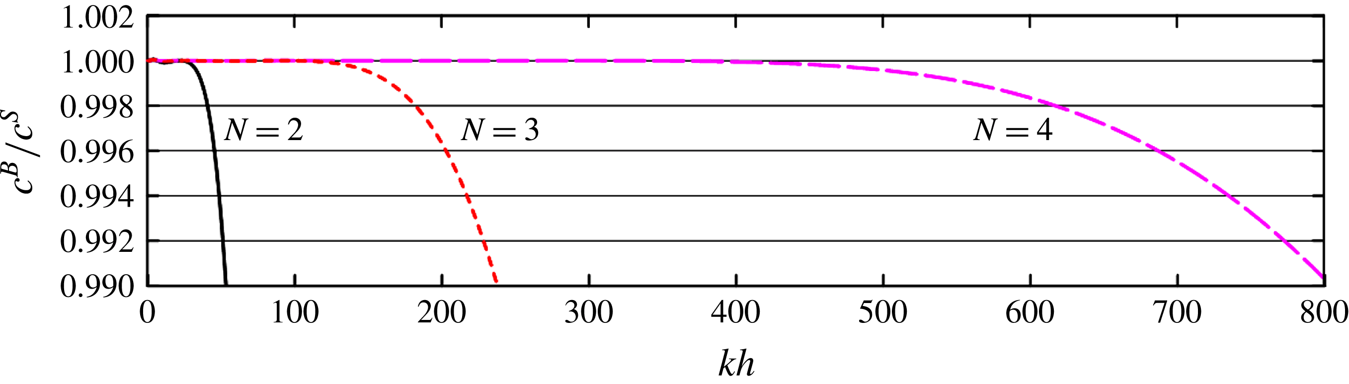
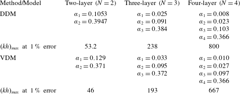
, 120 and 360 for the two-, three- and four-layer BT models, respectively. This approach has been used in previous studies (e.g. Simarro, Orfila & Galan Reference Simarro, Orfila and Galan2013; Liu & Fang Reference Liu and Fang2016) and is referred to as the dispersion dominant method (DDM) hereinafter. Table 1 lists the values of the coefficients that are calculated using this approach, and figure 2 presents the corresponding wave celerity results. Excellent accuracy is achieved by the multi-layer model in terms of the linear phase celerity as the number of layers increases. The maximum error of 1 % is achieved by the two-, three- and four-layer models and
 $kh$
values up to 53.2, 238 and 800, respectively. In addition, larger water depth limits can be obtained if the dispersion coefficients are determined using the maximum error of 1 % at the cost of lower accuracies in shallow-water regions.
Non-dimensional wave phase celerity of the multi-layer BT model (
 $N=2$
, 3 and 4) using the DDM. Here
 $c^{B}$
and
 $c^{S}$
denote the wave celerity obtained from the BT model and the Stokes solution, respectively.

Values of the dispersion coefficients determined using the dispersion dominant method (DDM) and velocity dominant method (VDM).

As an alternative approach for determining dispersion coefficients, the linear velocity dominant method (VDM) is used:
 $$\begin{eqnarray}\displaystyle F_{v}(\unicode[STIX]{x1D705})=\frac{1}{\unicode[STIX]{x1D705}}\int _{0}^{\unicode[STIX]{x1D705}}(F_{u}^{2}+F_{w}^{2})\,\text{d}(kh), & & \displaystyle\end{eqnarray}$$
where the velocity errors
 $F_{u}(\unicode[STIX]{x1D705})$
and
 $F_{w}(\unicode[STIX]{x1D705})$
are identical to those proposed by Madsen et al. (Reference Madsen, Bingham and Schäffer2003) and are expressed as
 $$\begin{eqnarray}\displaystyle F_{u}(kh)=\sqrt{\frac{1}{h}\int _{-h}^{0}\left(\frac{u(z)-u_{s}(z)}{u_{s}(0)}\right)^{2}\text{d}z}\quad \text{and}\quad F_{w}(kh)=\sqrt{\frac{1}{h}\int _{-h}^{0}\left(\frac{w(z)-w_{s}(z)}{w_{s}(0)}\right)^{2}\text{d}z}, & & \displaystyle \nonumber\\ \displaystyle & & \displaystyle\end{eqnarray}$$
where
 $u_{s}(0)$
and
 $w_{s}(0)$
are the maximum horizontal and vertical velocities at the still water level, respectively.
According to Madsen et al. (Reference Madsen, Bingham and Schäffer2003) and Liu & Fang (Reference Liu and Fang2016),
 $\unicode[STIX]{x1D705}$
is set to half the value of that used in the DDM, i.e.
 $\unicode[STIX]{x1D705}=15$
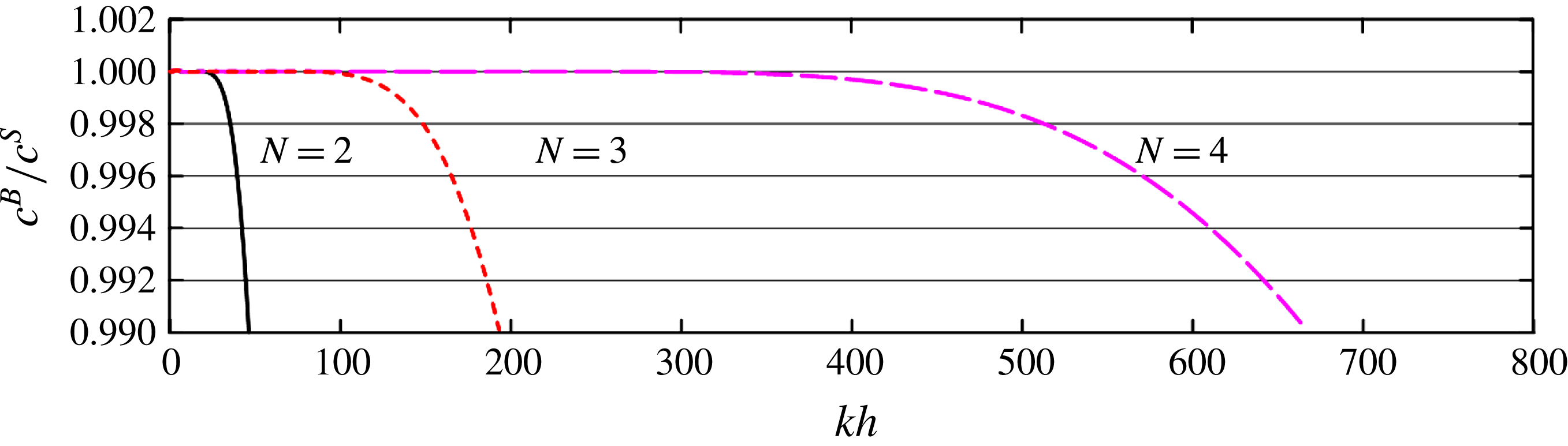
, 60 and 180 for the two-, three- and four-layer BT models, respectively. Table 1 lists the coefficients determined by the VDM, and figure 3 presents the corresponding wave celerities. The maximum applicable ranges of the multi-layer BT model obtained by the VDM are slightly reduced compared with those obtained by the DDM, but the dispersion determined by the VDM retains high accuracy. In addition, the overall velocity profiles obtained by the VDM are better than those produced by the DDM from shallow to deep water as shown in the following. Overall, the two-, three- and four-layer models are applicable up to
 $kh\approx 46$
, 193 and 667, respectively, with a maximum error of 1 %.
Non-dimensional wave phase celerities of the multi-layer BT model (
 $N=2$
, 3 and 4) obtained using the VDM. Here
 $c^{B}$
and
 $c^{S}$
denote the wave celerities obtained from the BT model and the Stokes solution, respectively.

3.1.2 Accuracy of the velocity profiles
Velocity profiles are important kinematic properties required for estimating wave impact on structures, and they are used to illustrate the performance of the present multi-layer BT model. The linear vertical profiles of the horizontal and vertical velocity expressions can be directly obtained from (2.20).
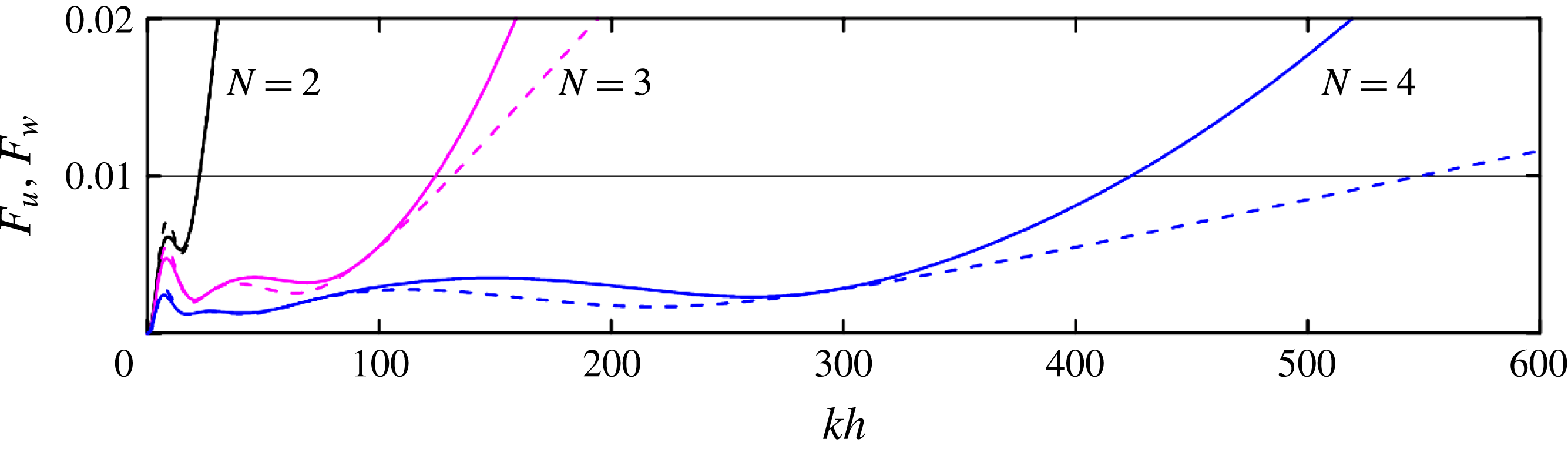
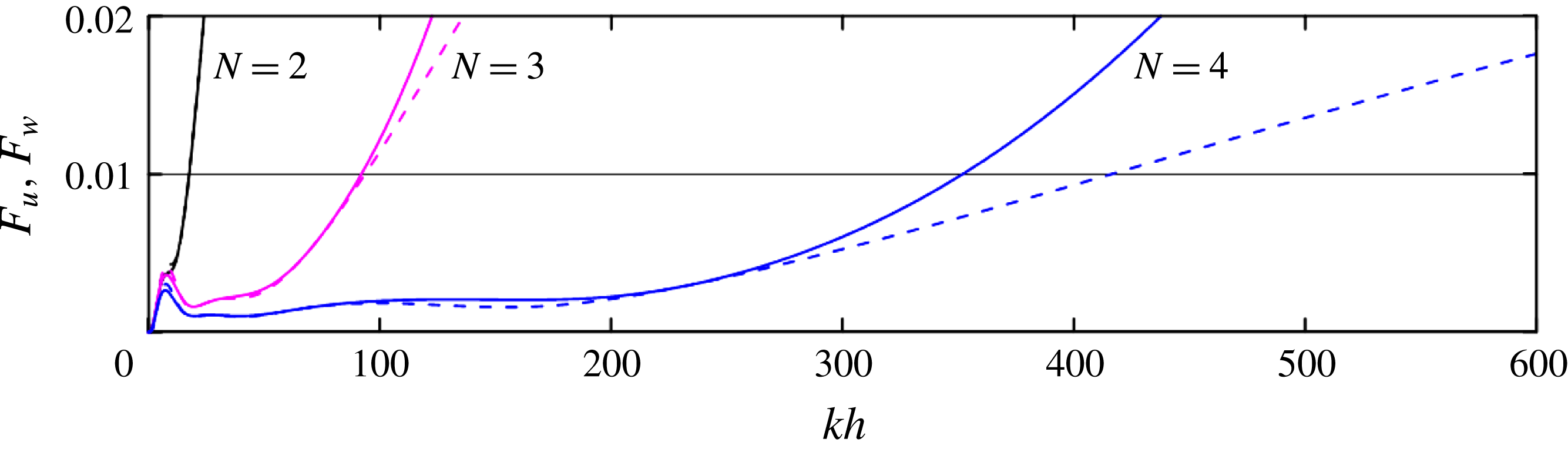
Figures 4 and 5 show the depth-integrated errors of the velocity components from (3.8) for the coefficients determined by the DDM and VDM, respectively. The accuracy of the models improves as
 $N$
increases. For the coefficients determined by the VDM, the applicable range increases from
 $kh\approx 17.6$
for
 $N=2$
, to
 $kh\approx 92.1$
for
 $N=3$
and to
 $kh\approx 352$
for
 $N=4$
, with a maximum error of 1 %. For the coefficients determined by the DDM, the applicable range increases from
 $kh\approx 22.4$
for
 $N=2$
, to
 $kh\approx 124.21$
for
 $N=3$
and to
 $kh\approx 423.8$
for
 $N=4$
, with a maximum error of 1 %. Figures 4 and 5 also show that the accuracy in the horizontal velocity profile is almost as good as that in the vertical velocity profile from the shallow-water depth to a fixed deep-water depth
 $(kh)_{max}$
. However, when the water depth exceeds this value, the error in the horizontal velocity increases faster than that in the vertical velocity. Compared with most conventional BT models, the accuracy of the horizontal velocity profile is much higher than that of the vertical profile because the same order of higher-order derivative terms in the horizontal velocities are retained in the vertical velocities in the multi-layer model.
Plot showing
 $F_{u}$
(solid line) and
 $F_{w}$
(dashed line) for the multi-layer BT model (
 $N=2$
, 3 and 4) obtained using the DDM.

Plot showing
 $F_{u}$
(solid line) and
 $F_{w}$
(dashed line) for the multi-layer BT model (
 $N=2$
, 3 and 4) obtained using the VDM.

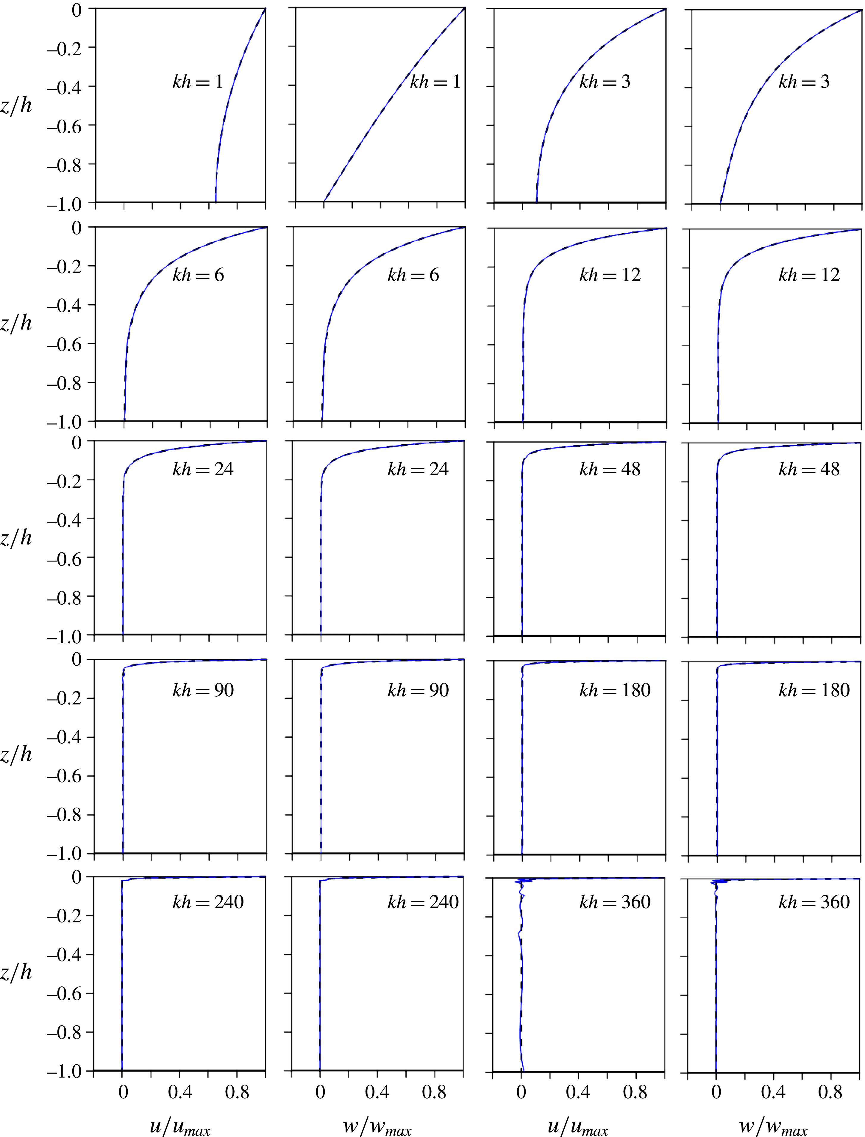
To further demonstrate the accuracy of the velocity field, the horizontal and vertical velocity profiles for a given water depth
 $kh$
are calculated within the applicable range of the models by using the coefficients determined by the VDM. Figure 6 compares the theoretical velocity results for the BT models and the target Stokes solution and shows that the four-layer BT model leads to highly accurate velocity profiles from shallow- to deep-water regions.
Vertical profiles of the horizontal and vertical velocities for eight
 $kh$
values. The dashed lines represent the linear theory solutions, and the solid lines denote those from the proposed four-layer BT model.

3.1.3 Accuracy of self–self interaction-generated second-order harmonics
The second-order solution, which reflects the leading-order nonlinear interactions, provides a benchmark for model assessments. Substituting (3.1) into the non-dimensionalized governing equations on a horizontal bottom and collecting the terms of
 $O(\unicode[STIX]{x1D700})$
yields the following:
 $$\begin{eqnarray}\displaystyle \left(\begin{array}{@{}ccccccccc@{}}m_{11}^{(2)} & m_{12}^{(2)} & m_{13}^{(2)} & 0 & 0 & 0 & 0 & 0 & 0\\ m_{21}^{(2)} & m_{22}^{(2)} & m_{23}^{(2)} & 0 & 0 & 0 & 0 & 0 & 0\\ 0 & m_{32}^{(2)} & m_{33}^{(2)} & m_{34}^{(2)} & m_{35}^{(2)} & 0 & 0 & 0 & 0\\ 0 & m_{42}^{(2)} & m_{43}^{(2)} & m_{44}^{(2)} & m_{45}^{(2)} & 0 & 0 & 0 & 0\\ 0 & 0 & 0 & m_{54}^{(2)} & m_{55}^{(2)} & m_{56}^{(2)} & m_{57}^{(2)} & 0 & 0\\ 0 & 0 & 0 & m_{64}^{(2)} & m_{65}^{(2)} & m_{66}^{(2)} & m_{67}^{(2)} & 0 & 0\\ 0 & 0 & 0 & 0 & 0 & m_{76}^{(2)} & m_{77}^{(2)} & m_{78}^{(2)} & m_{79}^{(2)}\\ 0 & 0 & 0 & 0 & 0 & m_{86}^{(2)} & m_{87}^{(2)} & m_{88}^{(2)} & m_{89}^{(2)}\\ 0 & 0 & 0 & 0 & 0 & 0 & 0 & m_{98}^{(2)} & m_{99}^{(2)}\end{array}\right)\left(\begin{array}{@{}c@{}}\unicode[STIX]{x1D702}_{2}\\ u_{12}\\ w_{12}\\ u_{22}\\ w_{22}\\ u_{32}\\ w_{32}\\ u_{42}\\ w_{42}\end{array}\right)=\left(\begin{array}{@{}c@{}}F_{1}\\ F_{2}\\ 0\\ 0\\ 0\\ 0\\ 0\\ 0\\ 0\\ \end{array}\right). & & \displaystyle\end{eqnarray}$$
Here
 $m_{11}^{(2)}=2\unicode[STIX]{x1D714}$
,
 $m_{21}^{(2)}=-2gk$
,
 $m_{98}^{(2)}=-sh2(\unicode[STIX]{x1D6FC}_{4}kh)$
and
 $m_{99}^{(2)}=ch2(\unicode[STIX]{x1D6FC}_{4}kh)$
, with
 $ch2(\unicode[STIX]{x1D706})=1+(2/5)(2\unicode[STIX]{x1D706})^{2}$
and
 $sh2(\unicode[STIX]{x1D706})=2\unicode[STIX]{x1D706}+(1/15)(2\unicode[STIX]{x1D706})^{3}$
; the other coefficients are obtained directly in a slightly different manner than the coefficients in (3.2). The expressions for
 $F_{i}$
(
 $i=1,2$
) are also lengthy and are therefore not included in this paper.
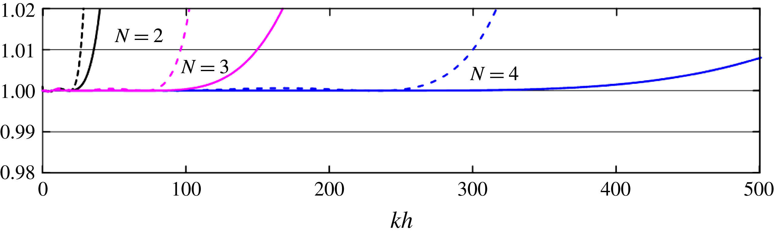
Only the VDM dispersive coefficients are considered here. Figure 7 shows the self–self harmonics of the four-layer BT model and shows that self–self interaction-generated super- and subharmonics become more accurate as the number of layers increases. The four-layer model is applicable up to
 $kh=300$
and presents a maximum error of 1 %, thereby demonstrating that the procedure proposed by Agnon et al. (Reference Agnon, Madsen and Schäffer1999) for decoupling the linear and nonlinear parts can also be used in the present multi-layer BT model.
Second order super- (solid line) and subharmonics (dashed line) of the proposed multi-layer BT model (
 $N=2$
, 3 and 4).

Third-order harmonics (solid line) and amplitude dispersion (dashed line) of the proposed multi-layer BT model (
 $N=2$
, 3 and 4).

3.1.4 Accuracy of the third-order harmonics
Substituting (3.1) into the non-dimensionalized governing equations on a horizontal bottom and collecting the terms of
 $O(\unicode[STIX]{x1D700}^{2})$
yields the following:
 $$\begin{eqnarray}\displaystyle & \displaystyle \left(\begin{array}{@{}ccccccccc@{}}m_{11}^{(3)} & m_{12}^{(3)} & m_{13}^{(3)} & 0 & 0 & 0 & 0 & 0 & 0\\ m_{21}^{(2)} & m_{22}^{(3)} & m_{23}^{(3)} & 0 & 0 & 0 & 0 & 0 & 0\\ 0 & m_{32}^{(3)} & m_{33}^{(3)} & m_{34}^{(3)} & m_{35}^{(3)} & 0 & 0 & 0 & 0\\ 0 & m_{42}^{(3)} & m_{43}^{(3)} & m_{44}^{(3)} & m_{45}^{(3)} & 0 & 0 & 0 & 0\\ 0 & 0 & 0 & m_{54}^{(3)} & m_{55}^{(3)} & m_{56}^{(3)} & m_{57}^{(3)} & 0 & 0\\ 0 & 0 & 0 & m_{64}^{(3)} & m_{65}^{(3)} & m_{66}^{(3)} & m_{67}^{(3)} & 0 & 0\\ 0 & 0 & 0 & 0 & 0 & m_{76}^{(3)} & m_{77}^{(3)} & m_{78}^{(3)} & m_{79}^{(3)}\\ 0 & 0 & 0 & 0 & 0 & m_{86}^{(3)} & m_{87}^{(3)} & m_{88}^{(3)} & m_{89}^{(3)}\\ 0 & 0 & 0 & 0 & 0 & 0 & 0 & m_{98}^{(3)} & m_{99}^{(3)}\end{array}\right)\left(\begin{array}{@{}c@{}}\unicode[STIX]{x1D702}_{33}\\ u_{133}\\ w_{133}\\ u_{233}\\ w_{233}\\ u_{333}\\ w_{333}\\ u_{433}\\ w_{433}\end{array}\right)=\left(\begin{array}{@{}c@{}}G_{1}\\ G_{2}\\ 0\\ 0\\ 0\\ 0\\ 0\\ 0\\ 0\end{array}\right), & \displaystyle \nonumber\\ \displaystyle & & \displaystyle\end{eqnarray}$$
 $$\begin{eqnarray}\displaystyle & \displaystyle \left(\begin{array}{@{}ccccccccc@{}}m_{11}^{(1)} & m_{12}^{(1)} & m_{13}^{(1)} & 0 & 0 & 0 & 0 & 0 & 0\\ m_{21}^{(1)} & m_{22}^{(1)} & m_{23}^{(1)} & 0 & 0 & 0 & 0 & 0 & 0\\ 0 & m_{32}^{(1)} & m_{33}^{(1)} & m_{34}^{(1)} & m_{35}^{(1)} & 0 & 0 & 0 & 0\\ 0 & m_{42}^{(1)} & m_{43}^{(1)} & m_{44}^{(1)} & m_{45}^{(1)} & 0 & 0 & 0 & 0\\ 0 & 0 & 0 & m_{54}^{(1)} & m_{55}^{(1)} & m_{56}^{(1)} & m_{57}^{(1)} & 0 & 0\\ 0 & 0 & 0 & m_{64}^{(1)} & m_{65}^{(1)} & m_{66}^{(1)} & m_{67}^{(1)} & 0 & 0\\ 0 & 0 & 0 & 0 & 0 & m_{76}^{(1)} & m_{77}^{(1)} & m_{78}^{(1)} & m_{79}^{(1)}\\ 0 & 0 & 0 & 0 & 0 & m_{86}^{(1)} & m_{87}^{(1)} & m_{88}^{(1)} & m_{89}^{(1)}\\ 0 & 0 & 0 & 0 & 0 & 0 & 0 & m_{99}^{(1)} & m_{99}^{(1)}\end{array}\right)\left(\begin{array}{@{}c@{}}\unicode[STIX]{x1D702}_{113}\\ u_{113}\\ w_{113}\\ u_{213}\\ w_{213}\\ u_{313}\\ w_{313}\\ u_{413}\\ w_{413}\end{array}\right) & \displaystyle \nonumber\\ \displaystyle & \displaystyle =\left(\begin{array}{@{}c@{}}f_{1}-\unicode[STIX]{x1D714}\unicode[STIX]{x1D714}_{13}\\ f_{2}+f_{3}\unicode[STIX]{x1D714}\unicode[STIX]{x1D714}_{13}\\ 0\\ 0\\ 0\\ 0\\ 0\\ 0\\ 0\end{array}\right). & \displaystyle\end{eqnarray}$$
Here
 $m_{11}^{(3)}=3\unicode[STIX]{x1D714}$
,
 $m_{21}^{(2)}=-3gk$
,
 $m_{98}^{(2)}=-sh3(\unicode[STIX]{x1D6FC}_{4}kh)$
and
 $m_{99}^{(2)}=ch3(\unicode[STIX]{x1D6FC}_{4}kh)$
, with
 $ch3(\unicode[STIX]{x1D706})=1+(2/5)(3\unicode[STIX]{x1D706})^{2}$
and
 $sh3(\unicode[STIX]{x1D706})=3\unicode[STIX]{x1D706}+(1/15)(3\unicode[STIX]{x1D706})^{3}$
; the other coefficients are obtained using (3.2). Because the terms on the right-hand side are tedious, they are not presented in this paper.
The values of
 $\unicode[STIX]{x1D702}_{33}$
and
 $\unicode[STIX]{x1D714}_{13}$
are obtained from (3.10) and (3.11), respectively, and they are compared with the analytical solution as follows (Skjelbreia & Hendrickson Reference Skjelbreia and Hendrickson1961):
 $$\begin{eqnarray}\displaystyle \unicode[STIX]{x1D702}_{33}^{s}=\frac{3}{64}k^{2}\unicode[STIX]{x1D702}_{1}^{3}\left(\frac{1+8\cosh ^{6}kh}{\sinh ^{6}kh}\right),\quad \unicode[STIX]{x1D714}_{13}^{s}=\frac{1}{16}k^{2}\unicode[STIX]{x1D702}_{1}^{2}\left(\frac{9\tanh ^{4}kh-10\tanh ^{2}kh+9}{\tanh ^{4}kh}\right). & & \displaystyle \nonumber\\ \displaystyle & & \displaystyle\end{eqnarray}$$
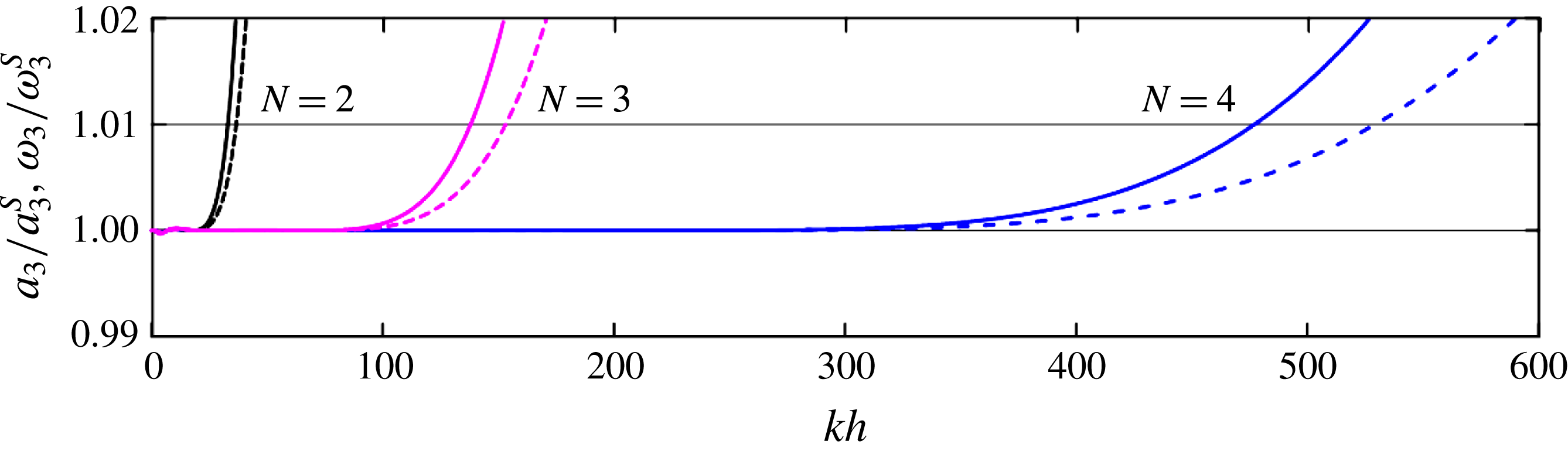
The results shown in figure 8 clearly indicate that the application range dramatically increases with increases in
 $N$
. In terms of the third-order harmonics and amplitude dispersion, the four-layer model is applicable up to a water depth of
 $kh=477$
and presents a 1 % tolerance error; to the best of the authors’ knowledge, this has not been previously achieved.
3.1.5 Accuracy of the sub- and superharmonics
The accuracy of the sub- and superharmonics for bichromatic waves is very important when verifying the applicability of BT models for simulating random waves (e.g. Madsen & Schäffer Reference Madsen and Schäffer1998; Gobbi & Kirby Reference Gobbi and Kirby2000; Madsen et al. Reference Madsen, Bingham and Liu2002; Lynett & Liu Reference Lynett and Liu2004a ; Liu & Fang Reference Liu and Fang2015, Reference Liu and Fang2016).
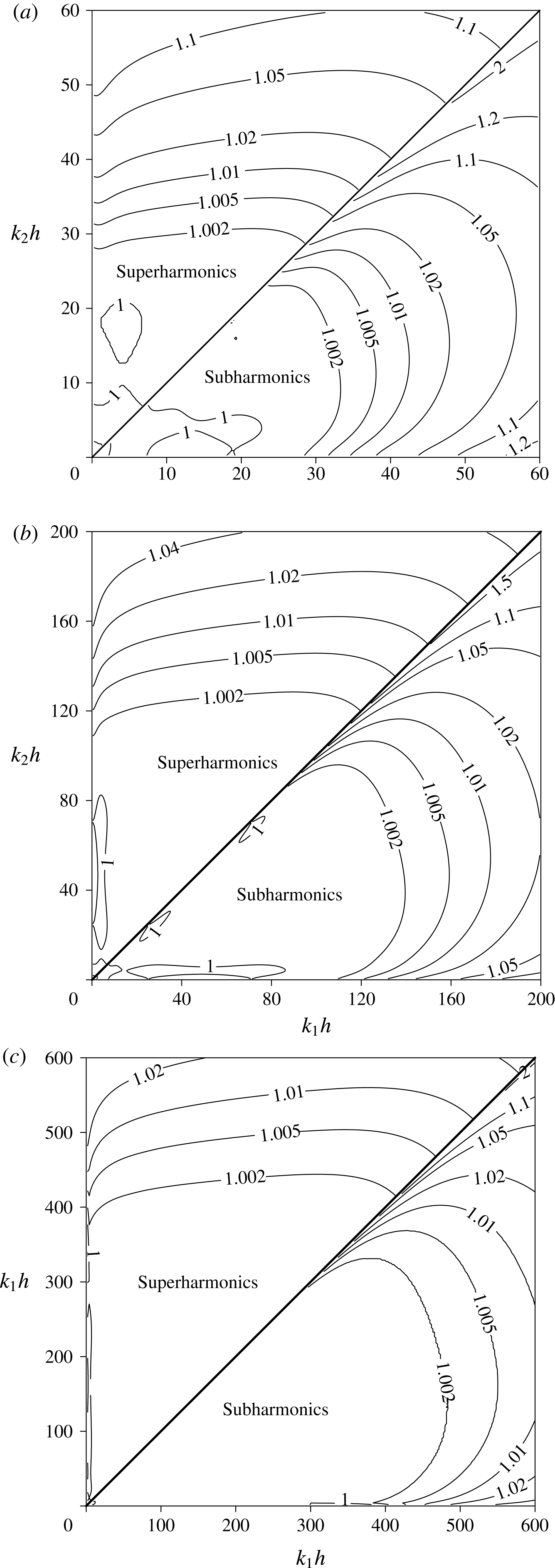
Based on the procedure proposed by Liu & Fang (Reference Liu and Fang2016), the second-order transfer functions of the two-, three- and four-layer BT models are obtained and presented in figure 9. Using the approach proposed by Agnon et al. (Reference Agnon, Madsen and Schäffer1999) and Madsen et al. (Reference Madsen, Bingham and Liu2002) based on the decoupling of linear and nonlinear properties in the multi-layer BT model, both the sub- and superharmonics show excellent accuracies, with 1 % tolerance errors
 $kh\approx 25$
, 90 and 300 for the two-, three- and four-layer BT models, respectively. However, the super- and subharmonics in conventional BT models show much lower accuracies. For example, with the fourth-order fully nonlinear BT equations derived by Zou & Fang (Reference Zou and Fang2008), the accuracy range for the sub- and superharmonics is valid only at
 $kh<1.0$
and presents a 1 % error.
Amplitudes of the sub- and superharmonic transfer functions for bichromatic waves of the proposed multi-layer BT model for
 $N=2$
(a),
 $N=3$
(b) and
 $N=4$
(c).

3.2 Accuracy of the linear shoaling amplitude
After omitting all nonlinear terms in the BT model, the following expressions for the surface elevation and velocities are obtained:
 $$\begin{eqnarray}\displaystyle \left.\begin{array}{@{}c@{}}\displaystyle \unicode[STIX]{x1D702}=A(x)\exp (\unicode[STIX]{x1D703}),\quad u_{i}^{\ast }=(B_{2i-1,1}(x)+\text{i}B_{2i-1,2}(x)h_{x})\exp (\unicode[STIX]{x1D703}),\\ \displaystyle w_{i}^{\ast }=(\text{i}B_{2i,1}(x)-B_{2i,2}(x)h_{x})\exp (\unicode[STIX]{x1D703}).\end{array}\right\} & & \displaystyle\end{eqnarray}$$
By inserting (3.13) into the linearized version of the multi-layer BT model (not presented in this study), a group of linear complex equations that incorporate real and imaginary parts are obtained. The linear dispersion and the shoaling gradient are solved by forcing the real and imaginary parts of the equations to zero, respectively. The shoaling gradient formula is obtained through the following procedure.
(1) The imaginary parts of the equations are used to obtain the expressions for
 $B_{2i-1,1}(x)$
(
 $i=1,4$
) through
 $(\unicode[STIX]{x2202}/\unicode[STIX]{x2202}x)(B_{2i-1,1})=B_{2i-1,1x}$
, where all
 $B_{2i-1,1x}$
are functions of the first-order derivatives of
 $A(x)$
,
 $k(x)$
and
 $h(x)$
(
 $A_{x}$
,
 $k_{x}$
and
 $h_{x}$
).
(2) By substituting
 $B_{2i-1,1x}$
into the real part of the equations, the relationship for
 $A_{x}$
,
 $k_{x}$
and
 $h_{x}$
is obtained as
 $$\begin{eqnarray}\displaystyle \unicode[STIX]{x1D70C}_{1}\frac{A_{x}}{A}+\unicode[STIX]{x1D70C}_{2}\frac{k_{x}}{k}+\unicode[STIX]{x1D70C}_{3}\frac{h_{x}}{h}=0. & & \displaystyle\end{eqnarray}$$
(3) The link between
 $k_{x}$
and
 $h_{x}$
is established by taking the partial derivative of the dispersion expression with respect to
 $\boldsymbol{x}$
:
 $$\begin{eqnarray}\displaystyle \unicode[STIX]{x1D70C}_{4}\frac{k_{x}}{k}+\unicode[STIX]{x1D70C}_{5}\frac{h_{x}}{h}=0. & & \displaystyle\end{eqnarray}$$
The expressions for
 $\unicode[STIX]{x1D70C}_{i}$
(
 $i=1$
to 5) will not be presented here due to their lengthy form.
Inserting (3.15) into (3.14) yields the following:
 $$\begin{eqnarray}\displaystyle \frac{A_{x}}{A}=-\unicode[STIX]{x1D6FE}^{b}\frac{h_{x}}{h}=-\frac{1}{\unicode[STIX]{x1D70C}_{1}}\left(\unicode[STIX]{x1D70C}_{3}-\unicode[STIX]{x1D70C}_{2}\frac{\unicode[STIX]{x1D70C}_{5}}{\unicode[STIX]{x1D70C}_{4}}\right)\frac{h_{x}}{h}. & & \displaystyle\end{eqnarray}$$
The shoaling coefficients are often determined by matching the shoaling gradients obtained from models and analytical solutions. However, such a practice may reduce the accuracy of the predicted shoaling amplitude in the numerical simulations (Chen & Liu Reference Chen and Liu1995; Galan et al.
Reference Galan, Simarro, Orfila, Simarro and Liu2012; Simarro et al.
Reference Simarro, Orfila and Galan2013; Liu & Fang Reference Liu and Fang2016). To avoid this issue, the following expression is employed to minimize the errors between the shoaling amplitudes of the BT model and the analytical solution (
 $A^{S}$
):
 $$\begin{eqnarray}\displaystyle \min \left|\frac{A}{A^{S}}-1\right|=\left|\exp \left(-\int _{0}^{\unicode[STIX]{x1D705}^{\ast }}\frac{\unicode[STIX]{x1D6FE}-\unicode[STIX]{x1D6FE}^{b}}{\unicode[STIX]{x1D705}^{\ast }}\,\text{d}\unicode[STIX]{x1D705}^{\ast }\right)-1\right|, & & \displaystyle\end{eqnarray}$$
where
 $\unicode[STIX]{x1D705}^{\ast }=k_{0}h$
, and
 $k_{0}$
is the wavenumber in deep water.
Values of the shoaling coefficients for the multi-layer model.

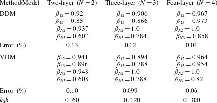
The coefficients determined by both the DDM and VDM are used in the above procedure, and
 $\unicode[STIX]{x1D705}^{\ast }=60$
, 120 and 300 is specified in the two-, three- and four-layer BT models, respectively. Table 2 lists the optimized shoaling coefficients. Within the optimization range of water depths, the errors are limited to 0.13 %, 0.12 % and 0.04 % using the DDM option, and to 0.1 %, 0.099 % and 0.06 % using the VDM option for the two-, three- and four-layer BT models, respectively. Thus, the shoaling amplitude shows excellent accuracy, and the difference between the VDM and DDM approaches is marginal.
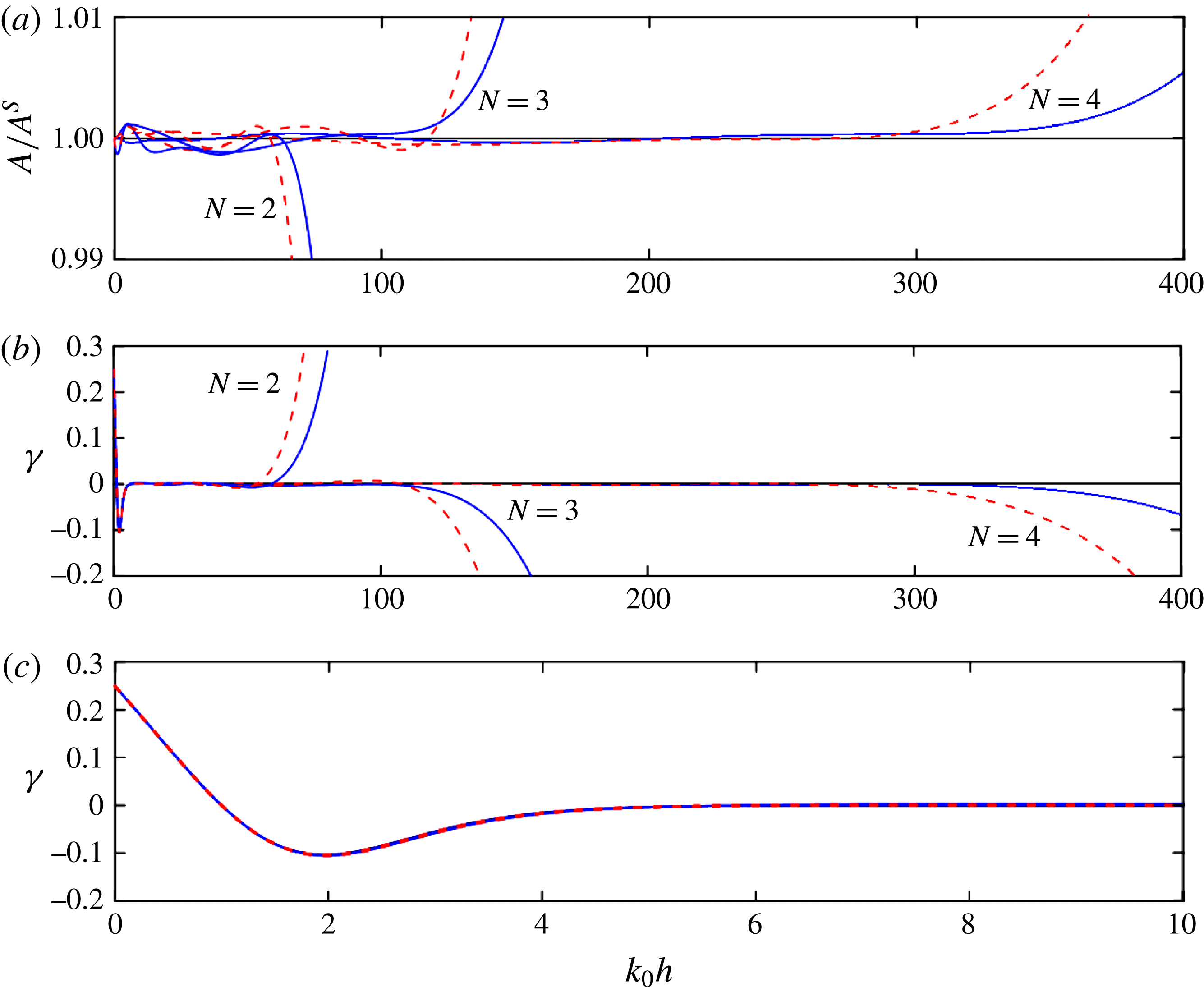
Figures 10(a) and 10(b) illustrate the shoaling amplitudes and shoaling gradients of the multi-layer model, respectively. Both the shoaling gradient and shoaling amplitude are consistent with the analytical solutions. Limited differences are observed in the shoaling gradient in shallow water over a wider
 $kh$
range of 400 to 0. Figure 10(c) presents an enlarged view of the range from 10 to 0, where only small differences are observed among the multi-layer models.
Shoaling amplitude (a) and shoaling gradient (b) using the DDM (solid line) and VDM (dashed line) of the proposed multi-layer BT model (
 $N=2$
, 3 and 4). (c) Enlargement of the shoaling gradient in the range of
 $0<k_{0}h<10$
.

4 Two sets of multi-layer Boussinesq models with different spatial derivatives
In the above derivation and analysis, the highest order of the spatial derivatives in the multi-layer model is limited to three (
 $n=3$
) to avoid numerical difficulties. In fact, higher-order spatial derivatives also contribute to the properties of the resulting model, and this point is illustrated by analysing the dispersion of the four-layer BT model using different highest orders of the derivatives (
 $n=2$
and 5). The derivation employs the same procedure as that presented in § 2, and the final velocity expressions are listed in appendix A.
Based on the procedures described in § 3, the dispersion coefficients obtained using the VDM approach are
 $\unicode[STIX]{x1D6FC}_{1}=0.022$
,
 $\unicode[STIX]{x1D6FC}_{2}=0.044$
,
 $\unicode[STIX]{x1D6FC}_{3}=0.111$
and
 $\unicode[STIX]{x1D6FC}_{4}=0.323$
for
 $n=2$
, and
 $\unicode[STIX]{x1D6FC}_{1}=0.0018$
,
 $\unicode[STIX]{x1D6FC}_{2}=0.0093$
,
 $\unicode[STIX]{x1D6FC}_{3}=0.0620$
and
 $\unicode[STIX]{x1D6FC}_{4}=0.4269$
for
 $n=5$
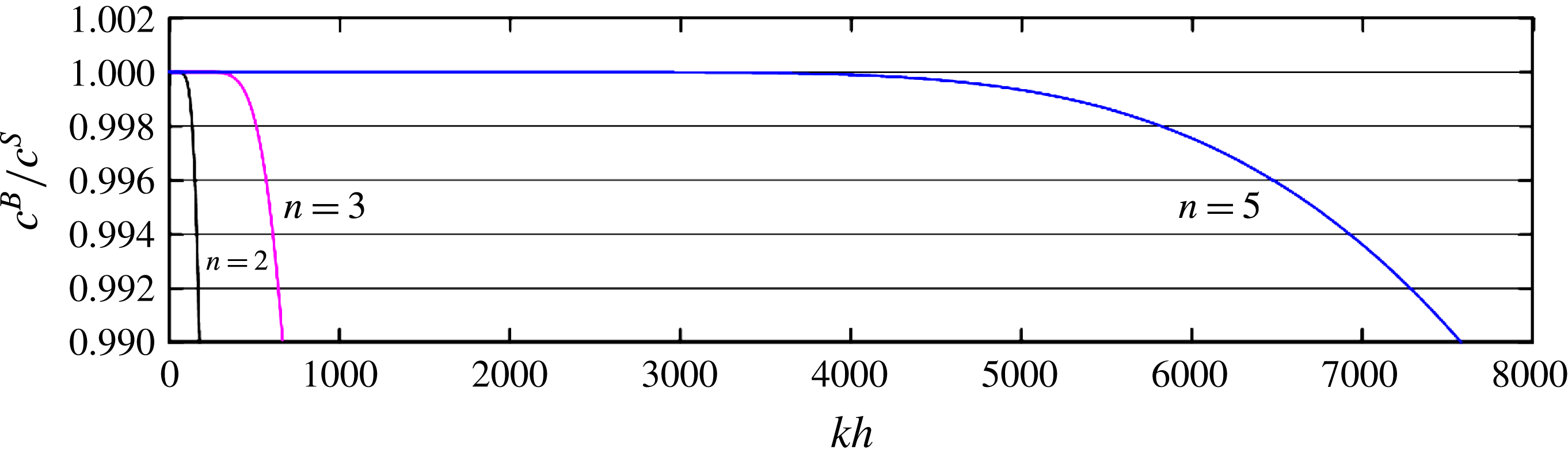
. Figure 11 compares the corresponding phase celerities in the four-layer BT model for
 $n=2$
, 3 and 5. The maximum applicable water depth is
 $kh=180$
, 667 and 7600 for the four-layer BT model with
 $n=2$
, 3 and 5, respectively, within a 1 % tolerance error. The accuracy of the phase celerity is greatly improved as
 $n$
increases. A similar effect of
 $n$
on the remaining properties of the multi-layer model is expected; however, further demonstrations are not presented in this paper.
Non-dimensional wave phase celerities for the four-layer BT model with
 $n=2$
, 3 and 5. Here
 $n$
is the highest order of the spatial derivatives in the multi-layer model; and
 $c^{B}$
and
 $c^{S}$
denote the wave celerities obtained from the BT model and the Stokes solution, respectively.

5 Numerical implementation and preliminary results
The vertical 2D version of the governing equations of the four-layer model consists of the following.
-
(i) The exact kinematic and dynamic surface conditions:
(5.1)and $$\begin{eqnarray}\displaystyle \frac{\unicode[STIX]{x2202}\unicode[STIX]{x1D702}}{\unicode[STIX]{x2202}t}=w_{\unicode[STIX]{x1D702}}-u_{\unicode[STIX]{x1D702}}\unicode[STIX]{x1D702}_{x} & & \displaystyle\end{eqnarray}$$
(5.2)
$$\begin{eqnarray}\displaystyle \frac{\unicode[STIX]{x2202}u_{\unicode[STIX]{x1D702}}}{\unicode[STIX]{x2202}t}=-g\unicode[STIX]{x1D702}_{x}-\frac{1}{2}(u_{\unicode[STIX]{x1D702}}^{2}+2u_{\unicode[STIX]{x1D702}}w_{\unicode[STIX]{x1D702}}\unicode[STIX]{x1D702}_{x})_{x}-\unicode[STIX]{x1D702}_{x}\frac{\unicode[STIX]{x2202}w_{\unicode[STIX]{x1D702}}}{\unicode[STIX]{x2202}t}+w_{\unicode[STIX]{x1D702}}(u_{\unicode[STIX]{x1D702}}\unicode[STIX]{x1D702}_{x})_{x}. & & \displaystyle\end{eqnarray}$$
-
(ii) The expressions for velocities on elevation of the free surface:
(5.3)and
$$\begin{eqnarray}\displaystyle u_{\unicode[STIX]{x1D702}}=u_{10}+\unicode[STIX]{x1D702}w_{10x}-{\textstyle \frac{1}{2}}\unicode[STIX]{x1D702}^{2}u_{10xx}-{\textstyle \frac{1}{6}}\unicode[STIX]{x1D702}^{3}w_{10xxx} & & \displaystyle\end{eqnarray}$$
(5.4)
$$\begin{eqnarray}\displaystyle w_{\unicode[STIX]{x1D702}}=w_{10}-\unicode[STIX]{x1D702}u_{10x}-{\textstyle \frac{1}{2}}\unicode[STIX]{x1D702}^{2}w_{10xx}+{\textstyle \frac{1}{6}}\unicode[STIX]{x1D702}^{3}u_{10xxx}. & & \displaystyle\end{eqnarray}$$
-
(iii) The velocity components defined on the still water level:
(5.5)and
$$\begin{eqnarray}\displaystyle u_{10}=u_{1}^{\ast }-\unicode[STIX]{x1D70E}_{1}u_{1xx}^{\ast }+\unicode[STIX]{x1D70E}_{2}w_{1x}^{\ast }-\unicode[STIX]{x1D70E}_{3}w_{1xxx}^{\ast }-\unicode[STIX]{x1D70E}_{4}u_{1x}^{\ast }+\unicode[STIX]{x1D70E}_{5}u_{1xxx}^{\ast }-\unicode[STIX]{x1D70E}_{6}w_{1xx}^{\ast } & & \displaystyle\end{eqnarray}$$
(5.6)
$$\begin{eqnarray}\displaystyle w_{10}=w_{1}^{\ast }-\unicode[STIX]{x1D70E}_{1}w_{1xx}^{\ast }-\unicode[STIX]{x1D70E}_{2}u_{1x}^{\ast }+\unicode[STIX]{x1D70E}_{3}u_{1xxx}^{\ast }-\unicode[STIX]{x1D70E}_{4}w_{1x}^{\ast }+\unicode[STIX]{x1D70E}_{5}w_{1xxx}^{\ast }+\unicode[STIX]{x1D70E}_{6}u_{1xx}^{\ast }. & & \displaystyle\end{eqnarray}$$
-
(iv) The velocity matching conditions on the interface between adjacent layers:
(5.7)
$$\begin{eqnarray}\displaystyle & & \displaystyle u_{2}^{\ast }-\unicode[STIX]{x1D70E}_{7}u_{2xx}^{\ast }+\unicode[STIX]{x1D70E}_{8}w_{2x}^{\ast }-\unicode[STIX]{x1D70E}_{9}w_{2xxx}^{\ast }-\unicode[STIX]{x1D70E}_{10}u_{2x}^{\ast }+\unicode[STIX]{x1D70E}_{11}u_{2xxx}^{\ast }(1-c_{1})-\unicode[STIX]{x1D70E}_{12}(1-{\textstyle \frac{1}{4}}c_{1})w_{2xx}^{\ast }\nonumber\\ \displaystyle & & \displaystyle \quad =u_{1}^{\ast }-\unicode[STIX]{x1D70E}_{1}u_{1xx}^{\ast }-\unicode[STIX]{x1D70E}_{2}w_{1x}^{\ast }+\unicode[STIX]{x1D70E}_{3}w_{1xxx}^{\ast }+\unicode[STIX]{x1D70E}_{4}u_{1x}^{\ast }-3\unicode[STIX]{x1D70E}_{5}u_{1xxx}^{\ast }-{\textstyle \frac{3}{2}}\unicode[STIX]{x1D70E}_{6}w_{1xx}^{\ast },\end{eqnarray}$$
(5.8)
$$\begin{eqnarray}\displaystyle & & \displaystyle w_{2}^{\ast }-\unicode[STIX]{x1D70E}_{7}w_{2xx}^{\ast }-\unicode[STIX]{x1D70E}_{8}u_{2x}^{\ast }+\unicode[STIX]{x1D70E}_{9}u_{2xxx}^{\ast }-\unicode[STIX]{x1D70E}_{10}w_{2x}^{\ast }+\unicode[STIX]{x1D70E}_{11}(1-c_{1})w_{2xxx}^{\ast }+\unicode[STIX]{x1D70E}_{12}(1-{\textstyle \frac{1}{4}}c_{1})u_{2xx}^{\ast }\nonumber\\ \displaystyle & & \displaystyle \quad =w_{1}^{\ast }-\unicode[STIX]{x1D70E}_{1}w_{1xx}^{\ast }+\unicode[STIX]{x1D70E}_{2}u_{1x}^{\ast }-\unicode[STIX]{x1D70E}_{3}u_{1xxx}^{\ast }+\unicode[STIX]{x1D70E}_{4}w_{1x}^{\ast }-3\unicode[STIX]{x1D6FD}_{13}\unicode[STIX]{x1D70E}_{5}w_{1xxx}^{\ast }+{\textstyle \frac{3}{2}}\unicode[STIX]{x1D6FD}_{12}\unicode[STIX]{x1D70E}_{6}u_{1xx}^{\ast },\end{eqnarray}$$
(5.9)
$$\begin{eqnarray}\displaystyle & & \displaystyle u_{3}^{\ast }-\unicode[STIX]{x1D70E}_{13}u_{3xx}^{\ast }+\unicode[STIX]{x1D70E}_{14}w_{3x}^{\ast }-\unicode[STIX]{x1D70E}_{15}w_{3xxx}^{\ast }-\unicode[STIX]{x1D70E}_{16}u_{3x}^{\ast }+\unicode[STIX]{x1D70E}_{17}(1-c_{2})u_{3xxx}^{\ast }-\unicode[STIX]{x1D70E}_{18}(1-{\textstyle \frac{1}{4}}c_{2})w_{3xx}^{\ast }\nonumber\\ \displaystyle & & \displaystyle \quad =u_{2}^{\ast }-\unicode[STIX]{x1D70E}_{7}u_{2xx}^{\ast }-\unicode[STIX]{x1D70E}_{8}w_{2x}^{\ast }+\unicode[STIX]{x1D70E}_{9}w_{2xxx}^{\ast }+\unicode[STIX]{x1D70E}_{10}u_{2x}^{\ast }-3\unicode[STIX]{x1D70E}_{11}(1+{\textstyle \frac{1}{3}}c_{1})u_{2xxx}^{\ast }\nonumber\\ \displaystyle & & \displaystyle \qquad -\,{\textstyle \frac{3}{2}}\unicode[STIX]{x1D70E}_{12}(1+{\textstyle \frac{1}{6}}c_{1})w_{2xx}^{\ast },\end{eqnarray}$$
(5.10)
$$\begin{eqnarray}\displaystyle & & \displaystyle w_{3}^{\ast }-\unicode[STIX]{x1D70E}_{13}w_{3xx}^{\ast }-\unicode[STIX]{x1D70E}_{14}u_{3x}^{\ast }+\unicode[STIX]{x1D70E}_{15}u_{3xxx}^{\ast }-\unicode[STIX]{x1D70E}_{16}w_{3x}^{\ast }+\unicode[STIX]{x1D70E}_{17}(1-c_{2})w_{3xxx}^{\ast }+\unicode[STIX]{x1D70E}_{18}(1-{\textstyle \frac{1}{4}}c_{2})u_{3xx}^{\ast }\nonumber\\ \displaystyle & & \displaystyle \quad =w_{2}^{\ast }-\unicode[STIX]{x1D70E}_{7}w_{2xx}^{\ast }+\unicode[STIX]{x1D70E}_{8}u_{2x}^{\ast }-\unicode[STIX]{x1D70E}_{9}u_{2xxx}^{\ast }+\unicode[STIX]{x1D70E}_{10}w_{2x}^{\ast }-3\unicode[STIX]{x1D70E}_{11}(1+{\textstyle \frac{1}{3}}c_{1})w_{2xxx}^{\ast }\nonumber\\ \displaystyle & & \displaystyle \qquad +\,{\textstyle \frac{3}{2}}(1+{\textstyle \frac{1}{6}}c_{1})\unicode[STIX]{x1D70E}_{12}u_{2xx}^{\ast },\end{eqnarray}$$
(5.11)
$$\begin{eqnarray}\displaystyle & & \displaystyle u_{4}^{\ast }-\unicode[STIX]{x1D70E}_{19}u_{4xx}^{\ast }+\unicode[STIX]{x1D70E}_{20}w_{4x}^{\ast }-\unicode[STIX]{x1D70E}_{21}w_{4xxx}^{\ast }-\unicode[STIX]{x1D70E}_{22}u_{4x}^{\ast }+\unicode[STIX]{x1D70E}_{23}(1-{\textstyle \frac{1}{4}}c_{3})u_{4xxx}^{\ast }-\unicode[STIX]{x1D70E}_{24}(1-{\textstyle \frac{1}{4}}c_{3})w_{4xx}^{\ast }\nonumber\\ \displaystyle & & \displaystyle \quad =u_{3}^{\ast }-\unicode[STIX]{x1D70E}_{13}u_{3xx}^{\ast }-\unicode[STIX]{x1D70E}_{14}w_{3x}^{\ast }+\unicode[STIX]{x1D70E}_{15}w_{3xxx}^{\ast }+\unicode[STIX]{x1D70E}_{16}u_{3x}^{\ast }-3\unicode[STIX]{x1D70E}_{17}(1+{\textstyle \frac{1}{3}}c_{2})u_{3xxx}^{\ast }\nonumber\\ \displaystyle & & \displaystyle \qquad -\,{\textstyle \frac{3}{2}}(1+{\textstyle \frac{1}{6}}c_{2})\unicode[STIX]{x1D70E}_{18}w_{3xx}^{\ast },\end{eqnarray}$$
(5.12)
$$\begin{eqnarray}\displaystyle & & \displaystyle w_{4}^{\ast }-\unicode[STIX]{x1D70E}_{19}w_{4xx}^{\ast }-\unicode[STIX]{x1D70E}_{20}u_{4x}^{\ast }+\unicode[STIX]{x1D70E}_{21}u_{4xxx}^{\ast }-\unicode[STIX]{x1D70E}_{22}w_{4x}^{\ast }+\unicode[STIX]{x1D70E}_{23}(1-c_{3})w_{4xxx}^{\ast }+\unicode[STIX]{x1D70E}_{24}(1-{\textstyle \frac{1}{4}}c_{3})u_{4xx}^{\ast }\nonumber\\ \displaystyle & & \displaystyle \quad =w_{3}^{\ast }-\unicode[STIX]{x1D70E}_{13}w_{3xx}^{\ast }+\unicode[STIX]{x1D70E}_{14}u_{3x}^{\ast }-\unicode[STIX]{x1D70E}_{15}u_{3xxx}^{\ast }+\unicode[STIX]{x1D70E}_{16}w_{3x}^{\ast }-3\unicode[STIX]{x1D70E}_{17}(1+{\textstyle \frac{1}{3}}c_{2})w_{3xxx}^{\ast }\nonumber\\ \displaystyle & & \displaystyle \qquad +\,{\textstyle \frac{3}{2}}(1+{\textstyle \frac{1}{6}}c_{2})\unicode[STIX]{x1D70E}_{18}u_{3xx}^{\ast }.\end{eqnarray}$$
-
(v) The kinematic bottom condition:
(5.13)
$$\begin{eqnarray}\displaystyle & & \displaystyle w_{4}^{\ast }-\unicode[STIX]{x1D70E}_{19}w_{4xx}^{\ast }+\unicode[STIX]{x1D70E}_{20}u_{4x}^{\ast }-\unicode[STIX]{x1D70E}_{21}u_{4xxx}^{\ast }+\unicode[STIX]{x1D70E}_{22}w_{4x}^{\ast }-3\unicode[STIX]{x1D6FD}_{N3}\unicode[STIX]{x1D70E}_{23}(1+{\textstyle \frac{1}{3}}c_{3})w_{4xxx}^{\ast }\nonumber\\ \displaystyle & & \displaystyle \qquad +\,{\textstyle \frac{3}{2}}\unicode[STIX]{x1D6FD}_{N2}\unicode[STIX]{x1D70E}_{24}(1+{\textstyle \frac{1}{6}}c_{3})u_{4xx}^{\ast }+h_{x}(u_{4}^{\ast }-\unicode[STIX]{x1D70E}_{19}u_{4xx}^{\ast }-\unicode[STIX]{x1D70E}_{20}w_{4x}^{\ast }+\unicode[STIX]{x1D70E}_{21}w_{4xxx}^{\ast })=0.\end{eqnarray}$$


Here
 $c_{1}=-(2\unicode[STIX]{x1D6FC}_{1}/(2\unicode[STIX]{x1D6FC}_{1}+\unicode[STIX]{x1D6FC}_{2}))$
,
 $c_{2}=-((2\unicode[STIX]{x1D6FC}_{1}+2\unicode[STIX]{x1D6FC}_{2})/(2\unicode[STIX]{x1D6FC}_{1}+2\unicode[STIX]{x1D6FC}_{2}+\unicode[STIX]{x1D6FC}_{3}))$
,
 $c_{3}~=$
 $-((2\unicode[STIX]{x1D6FC}_{1}+2\unicode[STIX]{x1D6FC}_{2}+2\unicode[STIX]{x1D6FC}_{3})/(2\unicode[STIX]{x1D6FC}_{1}+2\unicode[STIX]{x1D6FC}_{2}+2\unicode[STIX]{x1D6FC}_{3}+\unicode[STIX]{x1D6FC}_{4}))$
and
 $\unicode[STIX]{x1D70E}_{i}$
(
 $i=1,2,\ldots ,24$
) are given in appendix B. Note that the term related to
 $\unicode[STIX]{x1D702}_{tx}$
in (5.2) is rearranged using (5.1).
A numerical scheme similar to that used in the FUNWAVE model (Kirby et al.
Reference Kirby, Wei, Chen, Kennedy and Dalrymple1998) is employed to solve the above equations. A finite difference method with a structured quadrilateral mesh is used to approximate the spatial derivatives. The first- and second-order spatial derivatives of the unknown variables in the equations are discretized using a second-order scheme, and the rest are approximated with a fourth-order scheme. All third-order spatial derivatives are discretized with second-order accuracy. A composite fourth-order predictor–corrector Adams–Bashforth–Moulton integration scheme is employed for time marching. In the predictor stage, (5.1) and (5.2) are solved to obtain
 $\unicode[STIX]{x1D702}$
and
 $u_{\unicode[STIX]{x1D702}}$
, and those predicted values are then used to successively evaluate the horizontal velocities at the still water level
 $u_{10}$
and
 $u_{i}^{\ast }$
(
 $i=1,2,3,4$
) at the
 $z_{\unicode[STIX]{x1D6FC}i}$
locations. By substituting all predicted values into the right-hand side of (5.13), the vertical velocity at the fourth layer is obtained, and then the remaining vertical velocities from the bottom to the surface elevation are obtained successively by solving (5.12), (5.10), (5.8), (5.6) and (5.4). In the corrector stage, a similar process is iterated until the error between two successive evaluations reaches a predetermined norm, such as 0.00001. The convergence of iterations is accelerated by using an over-relaxation technique (Kirby et al.
Reference Kirby, Wei, Chen, Kennedy and Dalrymple1998).
In most of the following numerical experiments, sponge layers are employed at two ends of the computation domain to absorb the reflected waves, and the internal source method of Hsiao et al. (Reference Hsiao, Lynett, Hwung and Liu2005) is followed to generate waves in the numerical domain. The relaxation zone method proposed by Fuhrman (Reference Fuhrman2004) is employed to generate highly nonlinear incident waves with a sponge layer placed at the bottom end of the computational domain.
5.1 Regular linear and nonlinear wave evolution in deep waters of constant depth
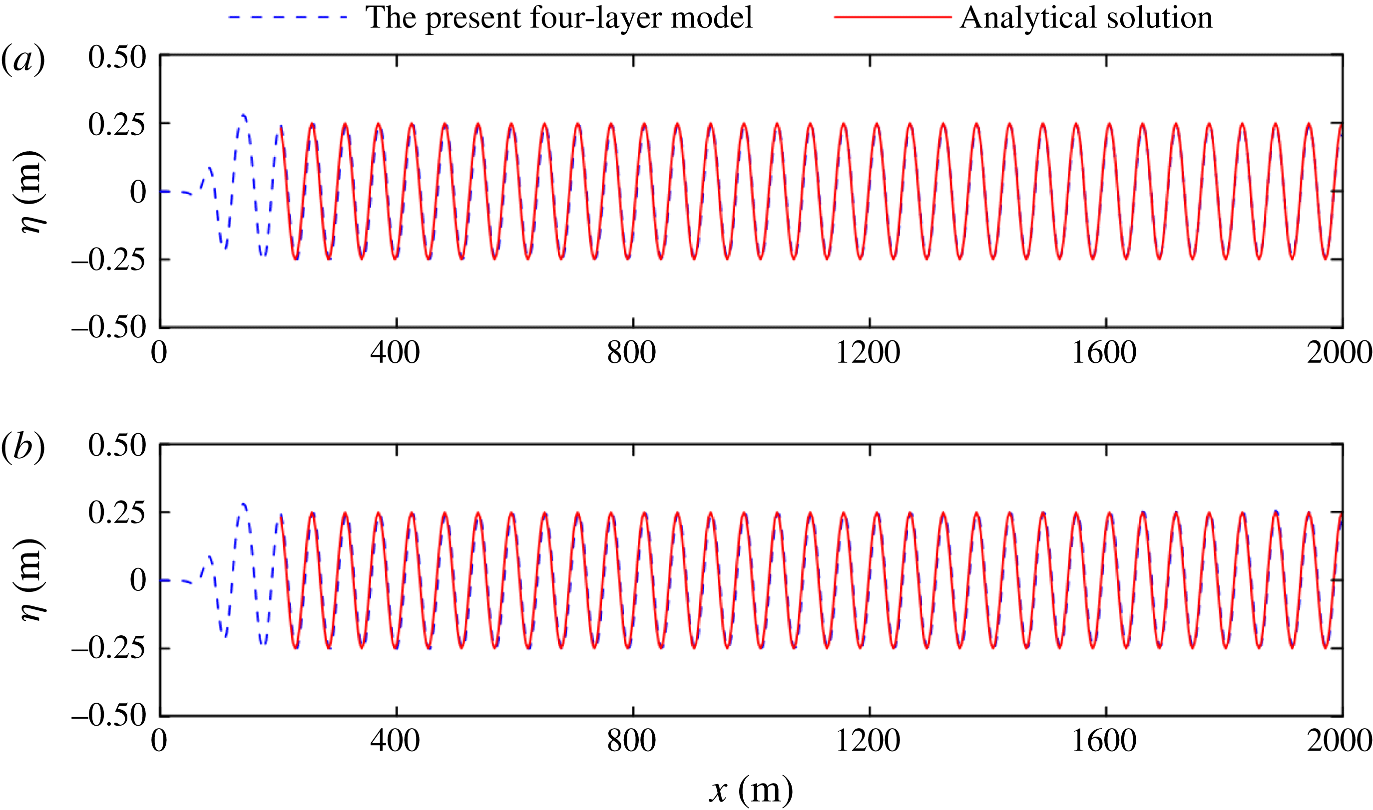
The first numerical test is conducted for the propagation of linear waves in deep water. In this case, dispersion dominates wave motion and the theoretical Stokes solution is employed as a benchmark reference. The incident wave period is 6 s, and the wave height is 0.5 m. The water depths are set to 56.2 m and 894.6 m (corresponding to
 $kh\approx 6.28$
and 100.0, respectively) in the numerical simulation. The centre of the internal source is located at
 $x=140$
m, and a space grid size of 3.513 m and time step of 0.2 s are used. Figure 12 compares the calculated surface elevations and analytical solutions, both of which show excellent consistency with regard to the wave shape, wave amplitude and phase. The relative errors in wavelength for these two cases are limited to only 0.2 %, which thereby showed the high dispersion accuracy. However, most Boussinesq models cannot accurately predict wave motion in deep water.
Comparisons of the free-surface elevations between the present model and the analytical solutions: (a)
 $kh=6.28$
and (b)
 $kh=100$
.

For highly nonlinear waves, the streamfunction method is employed to provide benchmark solutions to illustrate the applicability of the present model. Compared with the analytical solutions from Stokes theory, this approach is applicable over wide ranges of relative water depth and steepness with high accuracy (Chazel et al.
Reference Chazel, Benoit, Ern and Piperno2009). In the numerical simulation, the relaxation zone method (Fuhrman Reference Fuhrman2004) is used to generate the desired waves. For the selected application, the computational domain is
 $10L$
in length (
 $L$
is the wavelength), and a relaxation zone (covering 0–2
 $L$
) and sponge layer (covering 8–10
 $L$
) are imposed at the two lateral boundaries. A regular nonlinear wave with a period of
 $T=6.0$
s and wave height of
 $H=6.0$
m propagating over a still water depth of 360 m is simulated. The corresponding dimensionless water depth is
 $kh=36.66$
, and the wave steepness is
 $H/L=0.097$
(approximately 70 % of the theoretical maximum value of the steepness for a stable wave (Williams Reference Williams1985)), and these values represent a highly dispersive and nonlinear wave condition. The numerical simulation lasts
 $25T$
for a space grid size of
 $L/20$
and time step of
 $T/120$
.
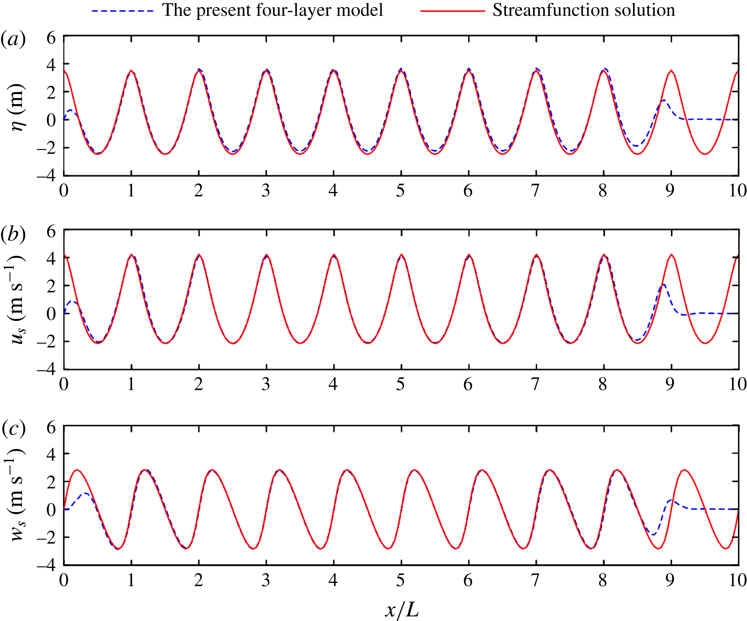
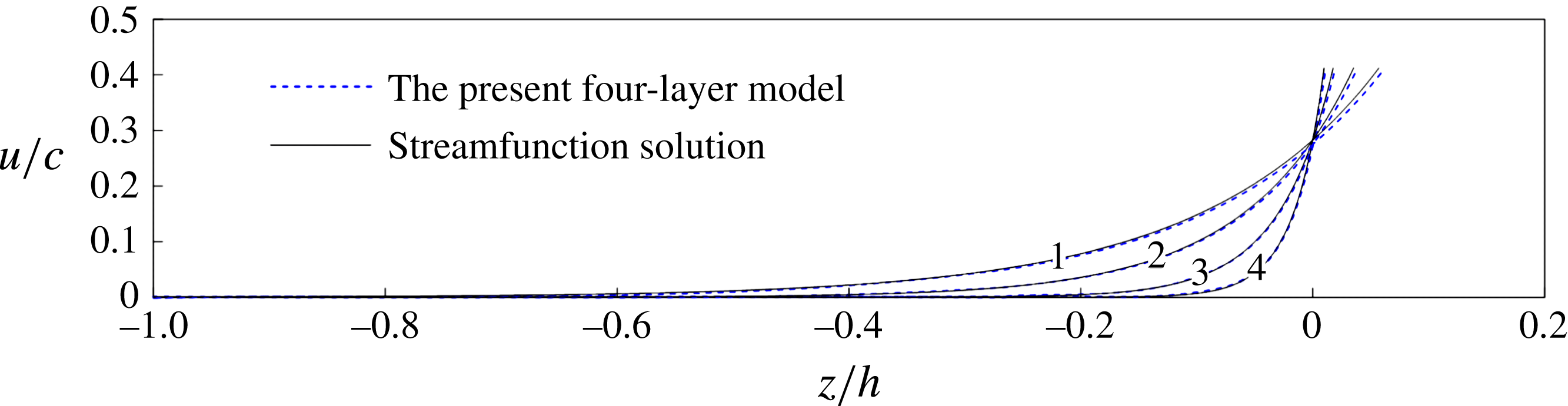
The calculated surface elevation and the velocities on the free-surface elevation are compared against the streamfunction solutions as shown in figure 13. With the exception of the slight upward shift of the free-surface elevations, the calculated results are consistent with the solutions from the streamfunction method, especially the calculated velocities on the free surface. The vertical distribution of the horizontal velocity is plotted in figure 14, which shows that the results are consistent. In the figure, we also present the results for other water depths of 60.173 m, 100 m and 200 m (
 $kh=6.28$
, 10.18 and 20.37, respectively). The comparison results are consistent. In summary, the model shows an excellent nonlinear performance.
Comparisons of the surface elevations (a) and horizontal (b) and vertical (c) velocities on the free surface between the present four-layer model and the streamfunction wave solution.

Vertical profiles of the horizontal velocities under the wave crest (where 1, 2, 3 and 4 stand for the cases of
 $kh=6.28$
, 10.18, 20.36 and 36.66, respectively).

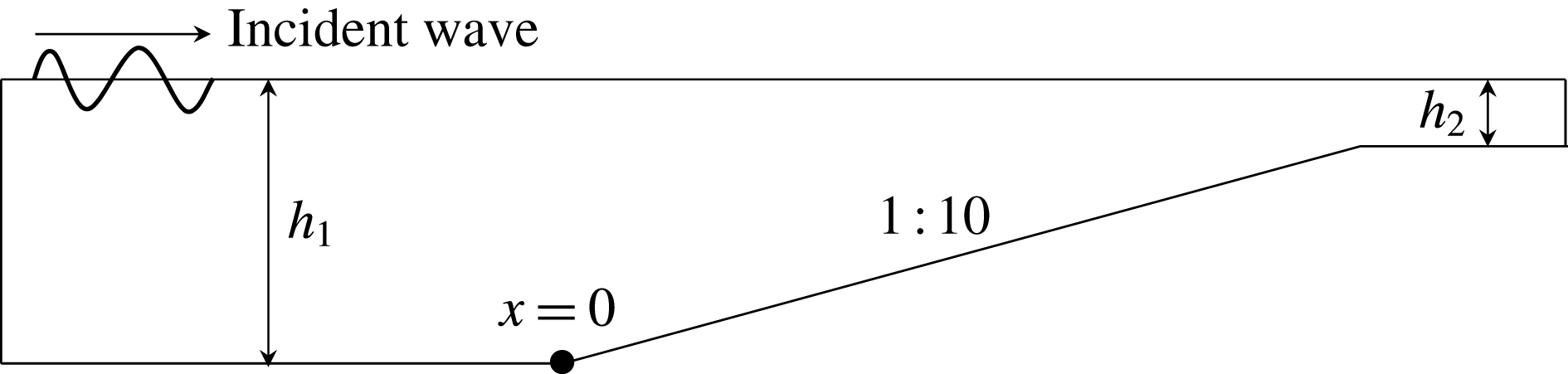
Sketch of the topography used for regular wave propagation and shoaling from deep water (
 $h_{1}$
) to shallow water (
 $h_{2}$
).

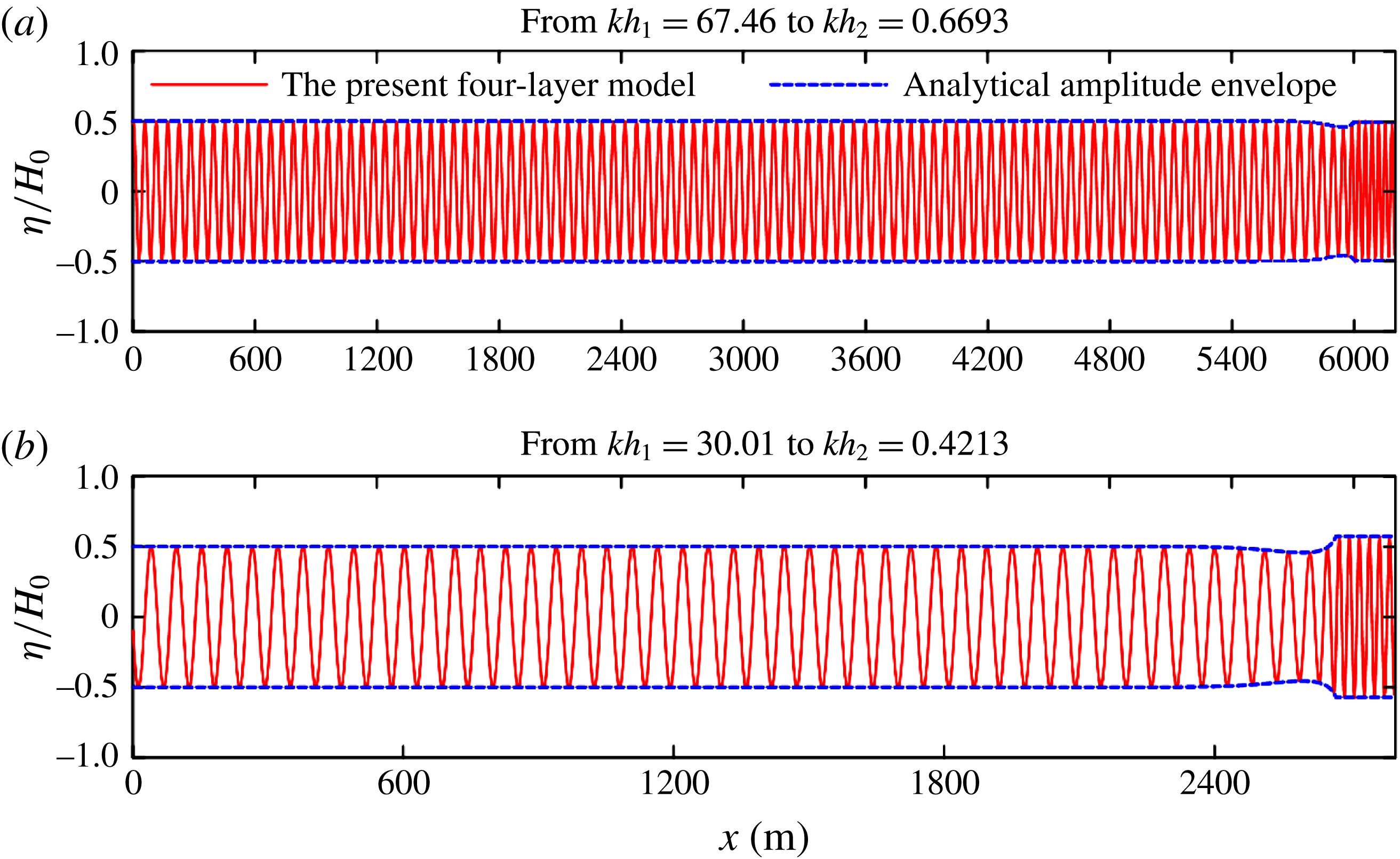
Calculated free-surface elevations and the corresponding analytical amplitude envelopes for linear waves shoaling over a 1 : 10 plane slope. Here
 $H_{0}$
denotes the incident wave amplitude.

5.2 Linear shoaling process from deep to shallow waters
To illustrate the wave shoaling performance of the model, two numerical simulations of regular waves with periods of
 $T=6.0$
s propagating over a 1 : 10 slope connected by deep water of depth
 $h_{1}$
and shallow water of depth
 $h_{2}$
are carried out with the topography being shown in figure 15. Without loss of generality and considering that the shoaling process of the gravity surface wave dominates in shallow waters, two numerical tests that cover the regime from deep water to a finite depth and from deep water to shallow water are conducted. In the first test, the linear wave propagates from
 $kh_{1}=67.46$
(
 $h_{1}=603.5$
m) to
 $kh_{2}=0.6693$
(
 $h_{2}=3.5$
m), and a space grid size of 3.6 m and time step of 0.2 s are used. In the second case, the water depth varies from
 $kh_{1}=30.01$
(
 $h_{1}=268.5$
m) to
 $kh_{2}=0.4213$
(
 $h_{2}=1.5$
m), and the grid size and time step are 1.5 m and 0.2 s, respectively. An ideal condition is represented by the two test cases covered in one test spanning the entire range of
 $0<kh<300$
. However, this condition is not computationally efficient because fine temporal and spatial resolutions are required in the shallow-water region to capture the smallest wave expected in the region, which will lead to unnecessarily fine temporal and spatial resolutions in the deep-water region because of the structured mesh used in this study. Figure 16(a,b) shows the calculated surface elevations together with the analytical solution of linear shoaling amplitude envelope, given by
 $$\begin{eqnarray}\displaystyle \frac{A_{x}}{A}=\frac{\displaystyle \frac{2kh}{\sinh 2kh}}{\left(1+\displaystyle 2kh\sinh 2kh\right)^{2}}\left[1+\frac{kh}{\sinh 2kh}(1-\cosh 2kh)\right]\frac{h_{x}}{h} & & \displaystyle\end{eqnarray}$$
in the Airy wave theory. Overall, the calculated results are consistent with the analytical solution, thus demonstrating the accuracy of the present model.
Schematic of the physical experiments of Luth, Kloman & Kitou (Reference Luth, Kloman and Kitou1994) (a) and Ohyama, Kiota & Tada (Reference Ohyama, Kiota and Tada1995) (b). All dimensions are expressed in metres.

5.3 Regular wave evolution over a submerged breakwater
The evolution of waves over a submerged breakwater is considered a complex process. The nonlinear interactions result in the transfer of energy from the leading wave component to higher harmonics as waves propagate on the front slope of the bar and steepen. As the water deepens, the nonlinear coupling of higher harmonics with the fundamental wave becomes progressively weaker at the lee side of the bar. Each Fourier component is released as a free wave with its own velocity, which results in a fairly complex process. An accurate prediction of this wave evolution process requires a model possessing high linear and nonlinear accuracies. Such predictions have been widely used as benchmark tests for validating BT models.
The model is validated against two physical experiments for regular wave propagation over (i) a submerged breakwater with a mild slope (Luth et al.
Reference Luth, Kloman and Kitou1994) and (ii) a steeper slope (Ohyama et al.
Reference Ohyama, Kiota and Tada1995). Figure 17 presents a sketch of the physical experiments. For case (a) in the experiment of Luth et al. (Reference Luth, Kloman and Kitou1994), the incident wave has a period of
 $T=2.02$
s and a wave height of
 $H=0.02$
m. The temporal and spatial resolutions employed in the simulation are 0.005 s and 0.03 m, respectively. The predicted wave elevations are consistent with those measured at all gauge locations in the experiments as shown in figure 18. The present model captures the above-mentioned complex process well. In the experiment of Ohyama et al. (Reference Ohyama, Kiota and Tada1995), the periods of the incident waves are
 $T=1.341$
, 2.012 and 2.683 s and the wave height is fixed at
 $H=0.05$
m. This test is more demanding than the former because the nonlinearity of the incident wave increases and the submerged sill changes sharply and presents a slope of 1 : 2. The temporal and spatial resolutions in the simulation are 0.005 s and 0.04 m, respectively. Again, the numerical results are consistent with the experimental data as shown in figure 19, demonstrating the good performance of the present model in simulating nonlinear waves.
Comparisons between the calculated surface elevations and the experimental data of Luth et al. (Reference Luth, Kloman and Kitou1994) at eight gauge locations for case (a).

Comparisons between the calculated surface elevations and the experimental data of Ohyama et al. (Reference Ohyama, Kiota and Tada1995) at two gauge locations for three cases: (a,b)
 $T=1.341$
s, (c,d)
 $T=2.012$
s, and (e,f)
 $T=2.683$
s.

One concern was that the model may encounter difficulties in shallow-water applications where the free surface cuts through the underlying layers, which did indeed happen in both of the test cases shown above. The free surface cut through the interface between the first layer and second layer in the area above the top of the sills. However, numerical instability did not occur, and the model still produced reasonably accurate results without any artificial interventions compared with the experimental results shown in figure 18 (
 $x=12.5$
m, 13.5 m) and figure 19 (#3). This finding is related to the unique nature of the computational velocities (pseudo-velocities) used in the multi-layer BT model. Moreover, the computational velocities are defined in the middle of each layer for the case of water at rest state (see figure 1), and the locations never change with time. These definitions hold regardless of where the free surface is or whether the free surface cuts through the underlying layers. All the values of the computational velocities (including those emergent from the instantaneous free surface) are used to evaluate/reconstruct the physical quantities in the numerical simulations, e.g. the velocities defined on the free surface
 $u_{\unicode[STIX]{x1D702}}$
and
 $w_{\unicode[STIX]{x1D702}}$
via (5.3) and (5.4).
6 Conclusions
In this study, a multi-layer irrotational BT model over a slow-varying bottom is proposed by generalizing the approach proposed by Liu & Fang (Reference Liu and Fang2016) in their two-layer BT model. The approach divides the simulation domain into multiple layers (Lynett & Liu Reference Lynett and Liu2004b ), replaces the velocities at an arbitrary water depth with pseudo-velocities (Madsen et al. Reference Madsen, Bingham and Liu2002), and decouples problems into linear and nonlinear parts (Agnon et al. Reference Agnon, Madsen and Schäffer1999). An important attribute of the proposed model is that it simulates linear and nonlinear properties with high accuracy, thereby increasing its applicability for highly nonlinear and extremely dispersive water waves. The main conclusions are summarized as follows.
-
(1) A high accuracy of linear dispersion is achieved. The two-, three- and four-layer models experienced 1 % errors up to
$kh\approx 53.2$
, 238 and 800, respectively. -
(2) The piecewise velocity used to match the exact linear Stokes wave velocity is directly responsible for the accuracy of the predicted velocity profiles.
-
(3) The present model generates highly accurate predictions of all nonlinear properties, such as the second-order harmonics for regular waves, the super- and subharmonics for bichromatic waves, and the third-order transfer function and dispersion amplitude. Specifically, the four-layer BT model exhibits extremely dispersive and fully nonlinear characteristics.
-
(4) The prediction accuracy of the shoaling property has also been greatly improved. The application range of the two-, three- and four-layer BT model is roughly
$kh=60$
, 120 and 300 and presents corresponding tolerances of 0.1 %, 0.1 % and 0.06 %. -
(5) Increasing the number of layers and the order of the derivatives leads to substantial improvements in the accuracy of linear and nonlinear property predictions, thereby providing a flexible option for the model in different applications.
-
(6) The fundamental properties of the present model have been demonstrated in a number of benchmark problems, and the performance of the model has been excellent, although numerical applications of the present model to a wide range of problems must be further investigated.


Acknowledgements
The authors would like to acknowledge the support from the National Key R&D Program of China (Project ID: 2016YFE0200100), and the National Natural Science Foundation of China (grant nos. 51779022, 51579034).
Appendix A. Expressions appearing in § 4 for two sets of multi-layer Boussinesq models with the highest order of the spatial derivatives
$n=2$
and
$n=5$


The velocities on the surface are expressed as follows.
For
 $n=5$
,
 $$\begin{eqnarray}\displaystyle \left.\begin{array}{@{}c@{}}\boldsymbol{u}_{\unicode[STIX]{x1D702}}=\boldsymbol{u}_{10}+\unicode[STIX]{x1D702}\unicode[STIX]{x1D735}w_{10}-{\textstyle \frac{1}{2}}\unicode[STIX]{x1D702}^{2}\unicode[STIX]{x1D6FB}^{2}\boldsymbol{u}_{10}-{\textstyle \frac{1}{6}}\unicode[STIX]{x1D702}^{3}\unicode[STIX]{x1D6FB}^{3}w_{10}+{\textstyle \frac{1}{24}}\unicode[STIX]{x1D702}^{4}\unicode[STIX]{x1D6FB}^{4}\boldsymbol{u}_{10}+{\textstyle \frac{1}{120}}\unicode[STIX]{x1D702}^{5}\unicode[STIX]{x1D6FB}^{5}w_{10},\\ w_{\unicode[STIX]{x1D702}}=w_{10}-\unicode[STIX]{x1D702}\unicode[STIX]{x1D735}\boldsymbol{\cdot }\boldsymbol{u}_{10}-\frac{1}{2}\unicode[STIX]{x1D702}^{2}\unicode[STIX]{x1D6FB}^{2}w_{10}+\frac{1}{6}\unicode[STIX]{x1D702}^{3}\unicode[STIX]{x1D6FB}^{3}\boldsymbol{u}_{10}+\frac{1}{24}\unicode[STIX]{x1D702}^{4}\unicode[STIX]{x1D6FB}^{4}w_{10}-\frac{1}{120}\unicode[STIX]{x1D702}^{5}\unicode[STIX]{x1D6FB}^{5}\boldsymbol{u}_{10}.\end{array}\right\} & & \displaystyle\end{eqnarray}$$
For
 $n=2$
,
 $$\begin{eqnarray}\displaystyle \left.\begin{array}{@{}c@{}}\boldsymbol{u}_{\unicode[STIX]{x1D702}}=\boldsymbol{u}_{10}+\unicode[STIX]{x1D702}\unicode[STIX]{x1D735}w_{10}-\frac{1}{2}\unicode[STIX]{x1D702}^{2}\unicode[STIX]{x1D6FB}^{2}\boldsymbol{u}_{10},\\ w_{\unicode[STIX]{x1D702}}=w_{10}-\unicode[STIX]{x1D702}\unicode[STIX]{x1D735}\boldsymbol{\cdot }\boldsymbol{u}_{10}-\frac{1}{2}\unicode[STIX]{x1D702}^{2}\unicode[STIX]{x1D6FB}^{2}w_{10}.\end{array}\right\} & & \displaystyle\end{eqnarray}$$
The velocity fields expressed in terms of the
 $N$
groups of velocities at
 $N$
depth locations are as follows:
 $$\begin{eqnarray}\displaystyle \boldsymbol{u}_{i}(\boldsymbol{x},z,t)=\mathop{\sum }_{j=0}^{n}\frac{1}{j!}(z-z_{\unicode[STIX]{x1D6FC}i})^{j}\left(\left.\frac{\unicode[STIX]{x2202}^{j}\boldsymbol{u}}{\unicode[STIX]{x2202}(jz)}\right|_{z=z_{\unicode[STIX]{x1D6FC}i}}\right),\quad \!w_{i}(\boldsymbol{x},z,t)=\mathop{\sum }_{j=0}^{n}\frac{1}{j!}(z-z_{\unicode[STIX]{x1D6FC}i})^{j}\left(\left.\frac{\unicode[STIX]{x2202}^{j}w}{\unicode[STIX]{x2202}(jz)}\right|_{z=z_{\unicode[STIX]{x1D6FC}i}}\right), & & \displaystyle \nonumber\\ \displaystyle & & \displaystyle\end{eqnarray}$$
The velocity fields expressed in terms of the
 $N$
groups of computation velocities are as follows:
 $$\begin{eqnarray}\displaystyle \left.\begin{array}{@{}c@{}}\displaystyle \boldsymbol{u}_{i}(\boldsymbol{x},z,t)=(\boldsymbol{J}_{01\unicode[STIX]{x1D6FC}i}+\unicode[STIX]{x1D735}z_{\unicode[STIX]{x1D6FC}i}\boldsymbol{J}_{11\unicode[STIX]{x1D6FC}i})\boldsymbol{u}_{i}^{\ast }+(\boldsymbol{J}_{02\unicode[STIX]{x1D6FC}i}+\unicode[STIX]{x1D735}z_{\unicode[STIX]{x1D6FC}i}\boldsymbol{J}_{12\unicode[STIX]{x1D6FC}i})w_{i}^{\ast },\\ \displaystyle w_{i}(\boldsymbol{x},z,t)=(\boldsymbol{J}_{01\unicode[STIX]{x1D6FC}i}+\unicode[STIX]{x1D735}z_{\unicode[STIX]{x1D6FC}i}\boldsymbol{J}_{11\unicode[STIX]{x1D6FC}1})w_{i}^{\ast }-(\boldsymbol{J}_{02\unicode[STIX]{x1D6FC}i}+\unicode[STIX]{x1D735}z_{\unicode[STIX]{x1D6FC}i}\boldsymbol{J}_{12\unicode[STIX]{x1D6FC}i})\boldsymbol{u}_{i}^{\ast },\end{array}\right\} & & \displaystyle\end{eqnarray}$$
where operators such as
 $\boldsymbol{J}_{01\unicode[STIX]{x1D6FC}i}$
are determined according to the choice of the highest derivatives.
For
 $n=2$
, these operators are
 $$\begin{eqnarray}\displaystyle \left.\begin{array}{@{}c@{}}\displaystyle \boldsymbol{J}_{01\unicode[STIX]{x1D6FC}i}=1-({\textstyle \frac{1}{2}}\unicode[STIX]{x1D713}^{2}-{\textstyle \frac{1}{6}}(\unicode[STIX]{x1D6FC}_{i}h)^{2})\unicode[STIX]{x1D6FB}^{2},\quad \boldsymbol{J}_{02\unicode[STIX]{x1D6FC}i}=\unicode[STIX]{x1D713}\unicode[STIX]{x1D735},\\ \displaystyle \boldsymbol{J}_{11\unicode[STIX]{x1D6FC}i}=\unicode[STIX]{x1D713}\unicode[STIX]{x1D735},\quad \boldsymbol{J}_{12\unicode[STIX]{x1D6FC}i}=\left(\frac{1}{3}(-\unicode[STIX]{x1D6FC}_{i}h)\unicode[STIX]{x1D713}\left(1+\frac{\unicode[STIX]{x1D735}d_{i-1}}{\unicode[STIX]{x1D735}z_{\unicode[STIX]{x1D6FC}i}}\right)+\unicode[STIX]{x1D713}^{2}\right)\unicode[STIX]{x1D6FB}^{2}.\end{array}\right\} & & \displaystyle\end{eqnarray}$$
For
 $n=5$
, these terms are
 $$\begin{eqnarray}\displaystyle \left.\begin{array}{@{}l@{}}\displaystyle \boldsymbol{J}_{01\unicode[STIX]{x1D6FC}i}=1-({\textstyle \frac{1}{2}}\unicode[STIX]{x1D713}^{2}-{\textstyle \frac{1}{18}}(\unicode[STIX]{x1D6FC}_{i}h)^{2})\unicode[STIX]{x1D6FB}^{2}+({\textstyle \frac{1}{24}}\unicode[STIX]{x1D713}^{4}-{\textstyle \frac{1}{36}}(\unicode[STIX]{x1D6FC}_{i}h)^{2}\unicode[STIX]{x1D713}^{2}+{\textstyle \frac{1}{504}}(\unicode[STIX]{x1D6FC}_{i}h)^{4})\unicode[STIX]{x1D6FB}^{4},\\ \displaystyle \boldsymbol{J}_{02\unicode[STIX]{x1D6FC}i}=\unicode[STIX]{x1D713}\unicode[STIX]{x1D735}-({\textstyle \frac{1}{6}}\unicode[STIX]{x1D713}^{3}-{\textstyle \frac{1}{18}}(\unicode[STIX]{x1D6FC}_{i}h)^{2}\unicode[STIX]{x1D713})\unicode[STIX]{x1D6FB}^{3}+({\textstyle \frac{1}{120}}\unicode[STIX]{x1D713}^{5}-{\textstyle \frac{1}{108}}(\unicode[STIX]{x1D6FC}_{i}h)^{2}\unicode[STIX]{x1D713}^{3}+{\textstyle \frac{1}{504}}(\unicode[STIX]{x1D6FC}_{i}h)^{4}\unicode[STIX]{x1D713})\unicode[STIX]{x1D6FB}^{5},\\ \displaystyle \boldsymbol{J}_{11\unicode[STIX]{x1D6FC}i}=\unicode[STIX]{x1D713}\unicode[STIX]{x1D735}\boldsymbol{\cdot }+\left(\frac{1}{18}(\unicode[STIX]{x1D6FC}_{i}h)^{2}\unicode[STIX]{x1D713}+\frac{1}{9}\unicode[STIX]{x1D6FC}_{i}h\unicode[STIX]{x1D713}^{2}\left(1+\frac{\unicode[STIX]{x1D735}d_{i-1}}{\unicode[STIX]{x1D735}z_{\unicode[STIX]{x1D6FC}i}}\right)-\frac{1}{2}\unicode[STIX]{x1D713}^{3}\right)\unicode[STIX]{x1D6FB}^{3},\\ \displaystyle \quad +\,\left(\frac{1}{24}\unicode[STIX]{x1D713}^{5}+\left(-\frac{1}{54}\unicode[STIX]{x1D6FC}_{i}h\unicode[STIX]{x1D713}^{4}+\frac{1}{126}(\unicode[STIX]{x1D6FC}_{i}h)^{3}\unicode[STIX]{x1D713}^{2}\right)\left(1+\frac{\unicode[STIX]{x1D735}d_{i-1}}{\unicode[STIX]{x1D735}z_{\unicode[STIX]{x1D6FC}i}}\right)\right.\\ \displaystyle \quad \left.-\,\frac{1}{36}(\unicode[STIX]{x1D6FC}_{i}h)^{2}\unicode[STIX]{x1D713}^{3}+\frac{1}{504}(\unicode[STIX]{x1D6FC}_{i}h)^{4}\unicode[STIX]{x1D713}\right)\unicode[STIX]{x1D6FB}^{5},\\ \displaystyle \boldsymbol{J}_{12\unicode[STIX]{x1D6FC}i}=\left(-\frac{1}{9}\unicode[STIX]{x1D6FC}_{i}h\unicode[STIX]{x1D713}(1+\frac{\unicode[STIX]{x1D735}d_{i-1}}{\unicode[STIX]{x1D735}z_{\unicode[STIX]{x1D6FC}i}})+\unicode[STIX]{x1D713}^{2}\right)\unicode[STIX]{x1D6FB}^{2}\\ \displaystyle \quad +\,\left(-\frac{1}{6}\unicode[STIX]{x1D713}^{4}+\left(\frac{1}{18}\unicode[STIX]{x1D6FC}_{i}h\unicode[STIX]{x1D713}^{3}-\frac{1}{126}(\unicode[STIX]{x1D6FC}_{i}h)^{3}\unicode[STIX]{x1D713}\right)\left(1+\frac{\unicode[STIX]{x1D735}d_{i-1}}{\unicode[STIX]{x1D735}z_{\unicode[STIX]{x1D6FC}i}}\right)+\frac{1}{18}(\unicode[STIX]{x1D6FC}_{i}h)^{2}\unicode[STIX]{x1D713}^{2}\right)\unicode[STIX]{x1D6FB}^{4}.\end{array}\right\} & & \displaystyle \nonumber\\ \displaystyle & & \displaystyle\end{eqnarray}$$
Appendix B. Expressions appearing in § 5 for vertical 2D version of the four-layer Boussinesq model
 $$\begin{eqnarray}\displaystyle & \displaystyle \left.\begin{array}{@{}c@{}}\unicode[STIX]{x1D70E}_{2}=\unicode[STIX]{x1D6FC}_{1}h,\quad \unicode[STIX]{x1D70E}_{8}=\unicode[STIX]{x1D6FC}_{2}h,\quad \unicode[STIX]{x1D70E}_{14}=\unicode[STIX]{x1D6FC}_{3}h,\quad \unicode[STIX]{x1D70E}_{20}=\unicode[STIX]{x1D6FC}_{4}h,\\ \unicode[STIX]{x1D70E}_{1}=\frac{2}{5}\unicode[STIX]{x1D70E}_{2}^{2},\quad \unicode[STIX]{x1D70E}_{7}=\frac{2}{5}\unicode[STIX]{x1D70E}_{8}^{2},\quad \unicode[STIX]{x1D70E}_{13}=\frac{2}{5}\unicode[STIX]{x1D70E}_{14}^{2},\quad \unicode[STIX]{x1D70E}_{19}=\frac{2}{5}\unicode[STIX]{x1D70E}_{20}^{2},\\ \unicode[STIX]{x1D70E}_{3}=\frac{1}{15}\unicode[STIX]{x1D70E}_{2}^{3},\quad \unicode[STIX]{x1D70E}_{9}=\frac{1}{15}\unicode[STIX]{x1D70E}_{8}^{3},\quad \unicode[STIX]{x1D70E}_{15}=\frac{1}{15}\unicode[STIX]{x1D70E}_{14}^{3},\quad \unicode[STIX]{x1D70E}_{21}=\frac{1}{15}\unicode[STIX]{x1D70E}_{20}^{2},\end{array}\right\} & \displaystyle\end{eqnarray}$$
 $$\begin{eqnarray}\displaystyle & \displaystyle \left.\begin{array}{@{}c@{}}\unicode[STIX]{x1D70E}_{4}=\unicode[STIX]{x1D6FC}_{1}^{2}hh_{x},\\ \unicode[STIX]{x1D70E}_{5}=\frac{1}{5}\unicode[STIX]{x1D6FC}_{1}^{4}h^{3}h_{x},\\ \unicode[STIX]{x1D70E}_{6}=\frac{4}{5}\unicode[STIX]{x1D6FC}_{1}^{3}h^{2}h_{x},\end{array}\right\} & \displaystyle\end{eqnarray}$$
 $$\begin{eqnarray}\displaystyle & \displaystyle \left.\begin{array}{@{}c@{}}\unicode[STIX]{x1D70E}_{10}=(2\unicode[STIX]{x1D6FC}_{1}+\unicode[STIX]{x1D6FC}_{2})\unicode[STIX]{x1D70E}_{8}h_{x},\\ \unicode[STIX]{x1D70E}_{16}=(2\unicode[STIX]{x1D6FC}_{1}+2\unicode[STIX]{x1D6FC}_{2}+\unicode[STIX]{x1D6FC}_{3})\unicode[STIX]{x1D70E}_{14}h_{x},\\ \unicode[STIX]{x1D70E}_{22}=(2\unicode[STIX]{x1D6FC}_{1}+2\unicode[STIX]{x1D6FC}_{2}+2\unicode[STIX]{x1D6FC}_{3}+\unicode[STIX]{x1D6FC}_{4})\unicode[STIX]{x1D70E}_{20}h_{x},\end{array}\right\} & \displaystyle\end{eqnarray}$$
 $$\begin{eqnarray}\displaystyle & \displaystyle \left.\begin{array}{@{}c@{}}\unicode[STIX]{x1D70E}_{11}=\frac{1}{5}\unicode[STIX]{x1D70E}_{8}^{2}\unicode[STIX]{x1D70E}_{10},\quad \unicode[STIX]{x1D70E}_{17}=\frac{1}{5}\unicode[STIX]{x1D70E}_{14}^{2}\unicode[STIX]{x1D70E}_{16},\quad \unicode[STIX]{x1D70E}_{23}=\frac{1}{5}\unicode[STIX]{x1D70E}_{20}^{2}\unicode[STIX]{x1D70E}_{22},\\ \unicode[STIX]{x1D70E}_{12}=\frac{4}{5}\unicode[STIX]{x1D70E}_{8}\unicode[STIX]{x1D70E}_{10},\quad \unicode[STIX]{x1D70E}_{18}=\frac{4}{5}\unicode[STIX]{x1D70E}_{14}\unicode[STIX]{x1D70E}_{16},\quad \unicode[STIX]{x1D70E}_{24}=\frac{4}{5}\unicode[STIX]{x1D70E}_{20}\unicode[STIX]{x1D70E}_{22}.\end{array}\right\} & \displaystyle\end{eqnarray}$$