
 p(ζ)
 ζ→±∞
 p~(ζ)



1. Introduction
The saddle-point approximation technique, also known as the method of steepest descent, has roots extending back to mathematical investigations in the 19th century. While Riemann (Reference Riemann1863) laid early groundwork for the asymptotic analysis of integrals, Debye (Reference Debye1909) is often credited with the first formal publication of the method applied to integrals in physics and applied mathematics. Although these early contributions are not explicit in the modern form, they established the foundation for the rigorous asymptotic techniques used today.
Building on these mathematical foundations, Daniels (Reference Daniels1954) pioneered the application of saddle-point approximations in statistics, presenting a comprehensive framework to approximate distributions of sums and other statistics with improved accuracy in the tails compared with classical methods. His work formalised the use of the cumulant generating function for deriving the saddle point and demonstrated its practical utility in statistical inference, thus establishing a cornerstone of modern asymptotic theory.
In the context of water-wave statistics, saddle-point methods have been rather sparsely employed. Machado (Reference Machado2003) developed a saddle-point approximation framework for probability density functions (PDFs) of the surface elevation in irregular seas, but did not obtain a closed-form expression, relying instead on implicit numerical solutions based on cumulant expansions. Butler et al. (Reference Butler, Machado and Rychlik2009) applied saddle-point methods to wave-crest distributions in mechanically generated bimodal seas, illustrating how third-order nonlinearities affect wave statistics with distance from the wavemaker. Wang (Reference Wang2024) extended saddle-point approaches to joint PDFs for rogue wave prediction under complex spectral conditions, enabling rapid assessment of extreme wave probabilities in nonlinear seas. These few studies highlight the method’s potential, but also its limited adoption in water-wave research to date.
The present work will focus on the classical integral formulation of Longuet-Higgins (Reference Longuet-Higgins1963), hereafter LH63, for the PDF of the surface elevation in nonlinear, irregular seas. His formulation is free of assumptions involving uni-directionality of the wave field or narrow-bandedness of the spectrum, as commonly made elsewhere (e.g. Tayfun Reference Tayfun1980; Tayfun & Alkhalidi Reference Tayfun and Alkhalidi2020). LH63 showed that to first order in the wave steepness, the PDF follows the Gaussian (normal) distribution. He likewise developed second-order (accounting for skewness) and third-order (additionally accounting for kurtosis) Gram–Charlier approximations, which have long been considered the standard of practice. Recently, Fuhrman et al. (Reference Fuhrman, Klahn and Zhai2023), hereafter FKZ, derived a previously unknown exact closed-form solution to the LH63 second-order integral in terms of the Airy function. They showed that the theoretical positive tail at this order is fundamentally heavier than predicted by the nonlinear approximations (both second- and third-order) of LH63. The tail behaviour is of both theoretical and practical interest, as it governs the probability of, for example, extreme surface elevations that will occur in rogue wave events. Klahn et al. (Reference Klahn, Zhai and Fuhrman2024) recently showed that solutions to the LH63 integral follow a previously unknown ordinary differential equation. From this they derived the theoretical form of the positive tails up to fifth order using the method of dominant balance, though their methodology was unable to obtain the multiplicative prefactors. In their appendix, Zhai et al. (Reference Zhai, Klahn, Onorato and Fuhrman2025) extended these results further to sixth order. Klahn et al. (Reference Klahn, Zhai and Fuhrman2024) and Zhai et al. (Reference Zhai, Klahn, Onorato and Fuhrman2025) utilised the tail asymptotics to generate sufficient boundary conditions, and generated PDFs through subsequent numerical integration of the ordinary differential equation. A problem common to the second- and third-order Gram–Charlier approximations of LH63, the second-order solution of FKZ as well as the numerically generated PDFs of Klahn et al. (Reference Klahn, Zhai and Fuhrman2024) and Zhai et al. (Reference Zhai, Klahn, Onorato and Fuhrman2025) is that all suffer from unphysical oscillations in the negative tail. Moreover, there are presently no closed-form theoretically based solutions to the third-order LH63 integral (either exact or approximate) which are consistent with the known tail asymptotics recently derived by Klahn et al. (Reference Klahn, Zhai and Fuhrman2024).
The present work will resolve the shortcomings discussed above by considering new saddle-point approximations to the LH63 integral truncated at various nonlinear orders. Considering each nonlinear order in sequence, we show that this type of approximation reproduces the Gaussian distribution at first order and provides a close match to the exact theory derived recently by FKZ at second order. We then go on to derive the principal novel result of this paper: a new closed-form solution for the third-order LH63 integral, accounting for both skewness and kurtosis. Importantly, this new third-order PDF is free of unphysical oscillations in the negative tail, a problem widely plaguing existing nonlinear PDFs, as described above. Being an approximation to the exact distribution, the new third-order PDF does not generally have unit integral, zero mean and unit variance, and its integral skewness and kurtosis do not match those implied by the input third and fourth cumulants. However, it will be established that these deficiencies can be remedied through a normalisation and (typically minor) adjustment to the input cumulants. The accuracy of the new third-order PDF will be established through comparison with challenging datasets stemming from irregular wave theory, a fully nonlinear numerical wave model as well as laboratory experiments.
The remainder of this paper is organised as follows. We briefly review saddle-point approximations of integrals having the form of present interest in § 2. Saddle-point approximations to the LH63 integral are then derived at first, second and third orders in § 3. Results from asymptotic analysis in both positive and negative tail limits are presented in § 4. The new third-order PDF is analysed in § 5, and a method of normalisation to enforce statistical properties consistent with the normalised surface elevation is presented. The accuracy of the new (normalised) third-order PDF is tested against the lower-order theories and selected theoretical, numerical and experimental datasets in § 6. Conclusions are finally drawn in § 7. A novel perturbation solution for obtaining asymptotic tail solutions is additionally presented in Appendix A, and employed to derive the theoretical positive and negative tails at fourth and fifth orders, which newly include the previously unknown multiplicative prefactors.
2. Review of saddle-point approximations
Considering a nonlinear, irregular sea with surface elevation (relative to the mean water level)
 $\eta$
having standard deviation
 $\sigma _\eta$
, LH63 showed that the PDF of the normalised free-surface elevation,
 $\zeta \equiv \eta / \sigma _\eta$
, can be expressed as the Fourier integral
 \begin{equation} p(\zeta )=\frac {1}{2\pi }\int _{-\infty }^{\infty }\exp \bigl (\phi (s)\bigr )\,\mathrm{d}s, \end{equation}
in which
 \begin{equation} \phi (s)=\mathrm{i}\zeta s + C(-\mathrm{i}s) \end{equation}
and
 $C(\boldsymbol{\cdot })$
denotes the cumulant generating function of
 $\zeta$
.
In order to approximate the integral (2.1), we employ the method of steepest descent (see e.g. § 6.6 of Bender & Orszag Reference Bender and Orszag1999). To that end, we first assume that the integration contour can be deformed from the real line to the path
 $\mathcal{C}$
in the complex plane along which
 ${\rm Im} {(\phi (s))}$
is constant and
 ${\rm Re} {(\phi (s))}$
decays in both directions away from the origin, such that
 \begin{equation} p(\zeta )=\frac {1}{2\pi }\int _{\mathcal{C}}\exp \bigl (\phi (s)\bigr )\,\mathrm{d}s. \end{equation}
Since the cumulant generating function is generally not known for large
 $|s|$
, this assumption cannot be rigorously justified. We note, however, that it corresponds to making the following two assumptions:
-
(i)
 $C$
is an analytic function in the subset of the complex plane containing both the real line and the path
$\mathcal{C}$
; and
-
(ii) the integrals of
$\exp (\phi (s))$
along the paths where
${\rm Re} {(\phi (s))} = \mathrm{constant}$
connecting the real line and
$\mathcal{C}$
vanish as
$|s|$
becomes large.





When combined with the residue theorem, (i) implies that the integral of
 $\exp (\phi (s))$
along the closed loop consisting of (a) the real line, (b) the path from the real line to
 $\mathcal{C}$
with
 ${\rm Re} {(\phi (s))} = \mathrm{constant}$
, (c)
 $\mathcal{C}$
in the opposite direction and (d) the path from
 $\mathcal{C}$
to the real line where
 ${\rm Re} {(\phi (s))} = \mathrm{constant}$
is exactly zero. Since (ii) guarantees that the contributions from the connection paths with
 ${\rm Re} {(\phi (s))} = \mathrm{constant}$
vanish, it follows that, under the present assumptions, (2.1) can be modified to (2.3).
Now, since
 ${\rm Im} {(\phi (s))}$
is constant along
 $\mathcal{C}$
and
 ${\rm Re} {(\phi (s))}$
decays in both directions for large
 $|s|$
, there must necessarily be at least one saddle point (Bender & Orszag Reference Bender and Orszag1999, p. 288),
 $\tilde {s}$
, on
 $\mathcal{C}$
such that
 \begin{equation} \phi '(\tilde {s})=0. \end{equation}
Near any such point, the phase admits the local expansion
 \begin{equation} \phi (s)=\phi (\tilde {s})+\frac {1}{2}\phi ''(\tilde {s})(s-\tilde {s})^2+ \cdots , \end{equation}
so that the deformed contour integral reduces at leading order to a Gaussian integral. This yields the standard saddle-point approximation for integrals of the form (2.1):
 \begin{equation} p(\zeta )\approx \frac {\exp (\phi (\tilde {s}))}{\sqrt {-2\pi \,\phi ''(\tilde {s})}}. \end{equation}
If more than one saddle contributes, the leading-order approximation is obtained by summing the corresponding saddle contributions:
 \begin{equation} p(\zeta )\approx \sum _k p_k(\zeta ) = \sum _k \frac {\exp (\phi (\tilde {s}_k))}{\sqrt {-2\pi \,\phi ''(\tilde {s}_k)}}. \end{equation}
The set of contributing saddles is determined by the geometry of
 $\phi (s)$
in the complex plane, as is discussed in what follows. The above should provide good approximations for
 $p(\zeta )$
provided that
 ${\rm Re} (\phi (s))$
decays rapidly near the contributing saddle point(s).
3. Saddle-point approximations of
$p(\zeta )$
at various nonlinear order

As mentioned in § 2, the cumulant generating function is not generally known. Following LH63, we will therefore approximate it locally by its cumulant expansion about
 $s=0$
:
 \begin{align} C(-\mathrm{i}s) & = \kappa _1(-\mathrm{i}s) + \frac {\kappa _2}{2}(-\mathrm{i}s)^2 + \frac {\kappa _3}{6}(-\mathrm{i}s)^3 + \frac {\kappa _4}{24}(-\mathrm{i}s)^4+ \cdots \nonumber \\ & = -\frac {s^2}{2}+\frac {\mathrm{i}\kappa _3}{6}s^3+\frac {\kappa _4}{24}s^4+ \cdots , \end{align}
where
 $\kappa _n$
is the
 $n$
th cumulant, and it has been invoked that
 $\kappa _1=0$
and
 $\kappa _2=1$
, since
 $\zeta$
has zero mean and unit variance. Invoking this within (2.2) leads to
 \begin{equation} \phi (s)= \mathrm{i}\zeta s-\frac {s^2}{2}+\frac {\mathrm{i}\kappa _3}{6}s^3+\frac {\kappa _4}{24}s^4+ \cdots . \end{equation}
The skewness is
 $\mathcal{S}=\langle \zeta ^3\rangle =\kappa _3=O(\varepsilon )$
, while the excess kurtosis is
 $\mathcal{K}-3=\kappa _4=O(\varepsilon ^2)$
, where
 $\mathcal{K}=\langle \zeta ^4\rangle$
is the kurtosis and
 $\varepsilon$
is a characteristic wave steepness (see equation (2.17) of LH63).
It is emphasised that the saddle-point approximations (2.6) or (2.7) were derived based on assumed properties of the exact analytically continued phase (2.2). In what follows, truncated versions of (3.2) will be used only to approximate the saddle-point locations and the local structure of
 $\phi (s)$
in the neighbourhood of contributing saddles. Specifically, truncated versions of (3.2) will be utilised to obtain quantities such as
 $\phi (\tilde {s})$
and
 $\phi ''(\tilde {s})$
, as needed to evaluate (2.6) or (2.7) at a given order in nonlinearity. As such, the convergence (or lack thereof) of the integral (2.1), with any truncated
 $\phi (s)$
from (3.2), on the original real axis has no bearing on the validity of any saddle-point approximations which follow. Obviously, since (3.2) stems from an expansion about
 $s=0$
, it is assumed that all relevant saddle points are sufficiently close to the origin in the complex plane.
3.1. First order
When truncated at leading (first, linear) order (3.2) is simply
 \begin{equation} \phi (s)=\mbox{i}\zeta s-\frac {s^2}{2}, \end{equation}
such that the lone saddle point is determined from (2.4):
 \begin{equation} \phi ^\prime (\tilde {s}) = \mbox{i}\zeta -\tilde {s} = 0, \end{equation}
yielding
 $\tilde {s}=\mbox{i}\zeta$
. Invoking this and that
 $\phi ^{\prime \prime }(\tilde {s})=-1$
within (2.6) then leads to
 \begin{equation} p(\zeta ) = \frac {1}{\sqrt {2\pi }}\exp \left (-\frac {\zeta ^2}{2}\right ), \end{equation}
which corresponds to the Gaussian (normal) distribution. In this case, the saddle-point approximation yields the well-known exact result, first derived by LH63. Hence, in the present case, the equals sign is invoked above.
3.2. Second order
Truncated at second order, (3.2) incorporates the skewness:
 \begin{equation} \phi (s)=\mbox{i}\zeta s -\frac {s^2}{2} + \frac {\mbox{i}\kappa _3}{6} s^3. \end{equation}
The saddle points now correspond to those where
 \begin{equation} \phi ^\prime (\tilde {s}) = \mbox{i}\zeta -\tilde {s} + \frac {\mbox{i}\kappa _3}{2}\tilde {s}^2=0, \end{equation}
yielding
 \begin{equation} \{\tilde {s}_1,\tilde {s}_2\}=\frac {\mbox{i}(-1 \pm \sqrt {\lambda })}{\kappa _3}, \end{equation}
where
 \begin{equation} \lambda =1+2\zeta \kappa _3. \end{equation}
The second derivative at the saddle point is
 \begin{equation} \phi ^{\prime \prime }(\tilde {s})=\mbox{i}\kappa _3 \tilde {s} - 1. \end{equation}
Invoking all of the above into (2.6) leads to the two options
 \begin{equation} \{p_1(\zeta ),p_2(\zeta )\}\approx \frac {1}{\sqrt {2\pi }\sqrt {\pm \lambda ^{1/2}}}\exp \left (\frac {(\sqrt {\lambda } \mp 1)(\sqrt {\lambda }\mp 1\mp 4\zeta \kappa _3)}{6\kappa _3^2} \right ). \end{equation}
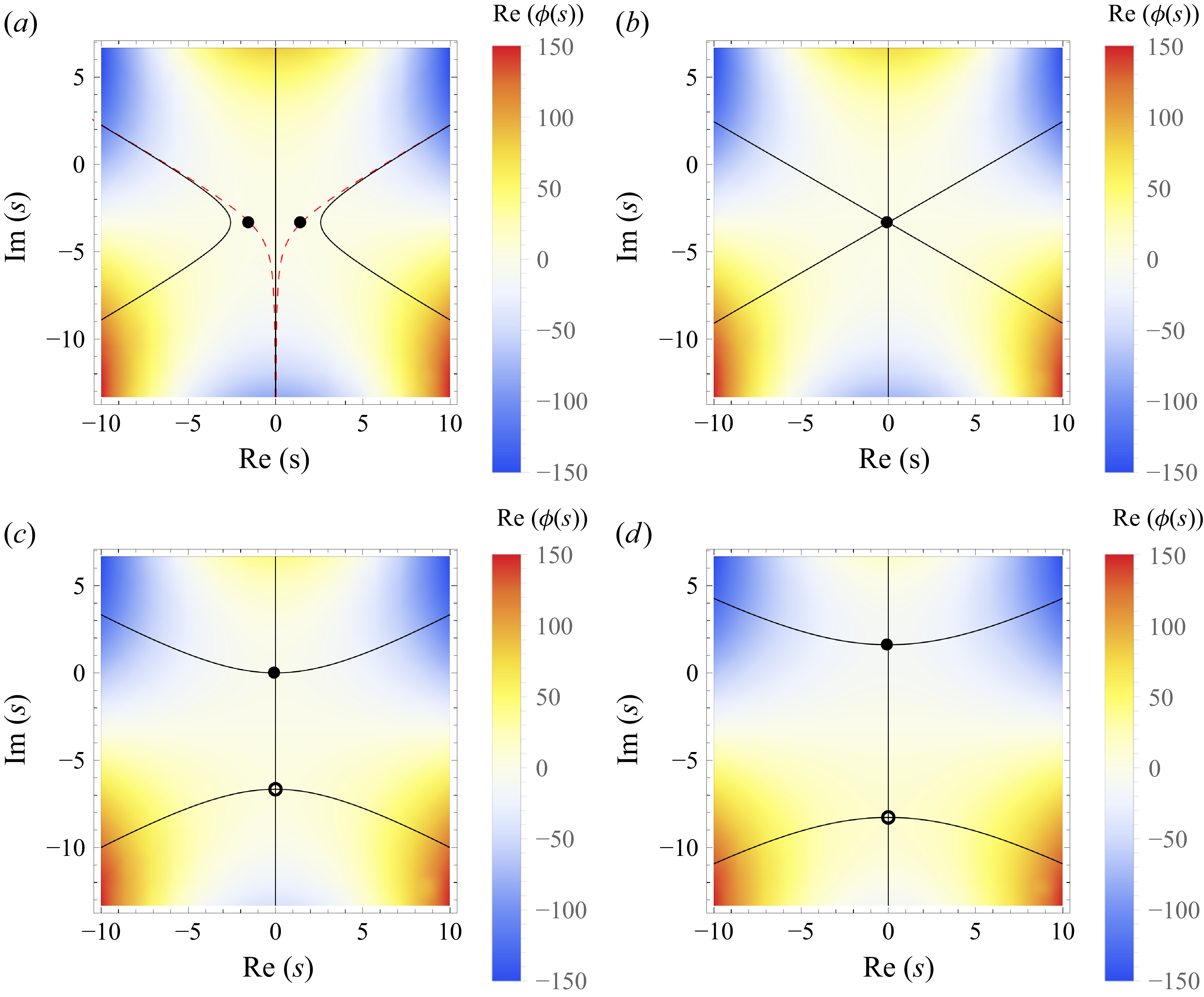
Plots showing the second-order saddle-point positions (black circles) in the complex plane, contours where
 ${\rm Im} (\phi (s))=0$
(full black lines) as well as
 ${\rm Re} (\phi (s))$
(colours). Results use fixed
 $\kappa _3=0.3$
with (
 $a$
)
 $\zeta =-2$
, (
 $b$
)
 $\zeta =\zeta _{crit}=-1.\overline {6}$
, (
 $c$
)
 $\zeta =0$
and (
 $d$
)
 $\zeta =2$
. The dashed red lines in (
 $a$
) depict additional contours where
 ${\rm Im} (\phi (s))={\rm Im} (\phi (\tilde {s}))\neq 0$
.

Note that both contain singularities where
 $\lambda =0$
, corresponding to
 $\zeta =\zeta _{crit}= -1/(2\kappa _3)$
.
To determine which saddle points contribute we will inspect their position in relation to the behaviour of the truncated
 $\phi (s)$
in the complex plane. Figure 1 exemplifies the complex plane with fixed
 $\kappa _3=0.3$
and various
 $\zeta$
values, as indicated in the caption. Colour density plots for
 ${\rm Re} (\phi (s))$
are shown, as well as the contours where
 ${\rm Im} (\phi (s))=0$
(full lines), with the saddle points shown as filled (contributing) or open (non-contributing) circles, as will be explained further below. For
 $\zeta \gt \zeta _{crit}$
(figure 1
c,d) the saddle points are purely imaginary and lie directly on these contours. It is clear that the uppermost saddle point (
 $\tilde {s}_1$
) lies on the contour representing the path of steepest descent (
 ${\rm Re} (\phi (s))$
decays very rapidly along this contour), and will thus be the only contributor; the contour passing through the lower saddle point (
 $\tilde {s}_2$
) actually represents the path of steepest ascent. At
 $\zeta =\zeta _{crit}$
(figure 1
b) the two saddle points coalesce. For
 $\zeta \lt \zeta _{crit}$
(figure 1
a), the saddle points bifurcate, and no longer lie on a
 ${\rm Im} (\phi (s))=0$
contour. Both must contribute in order for the integration path to span the entire real axis, but with the integration made along the contours where
 ${\rm Im} (\phi (\tilde {s}))= \mathrm{constant}$
, additionally depicted as the red dashed lines. As
 $\phi (s)$
has non-zero imaginary part along these contours, oscillations will inevitably occur in the negative tail. For
 $\zeta \lt \zeta _{crit}$
,
 $p_1(\zeta )$
and
 $p_2(\zeta )$
, in fact, form complex conjugates, and hence once added together as in (2.7) form a real-valued approximation of the PDF. The saddle-point approximation to the PDF at second order is thus
 \begin{equation} p(\zeta ) \approx \begin{cases} p_1(\zeta ) + \text{c.c.}, \hspace {0.5cm} \zeta \lt \zeta _{crit},\\ p_1(\zeta ), \hspace {1.4cm} \zeta \geqslant \zeta _{crit}, \end{cases} \end{equation}
where
 $\text{c.c.}$
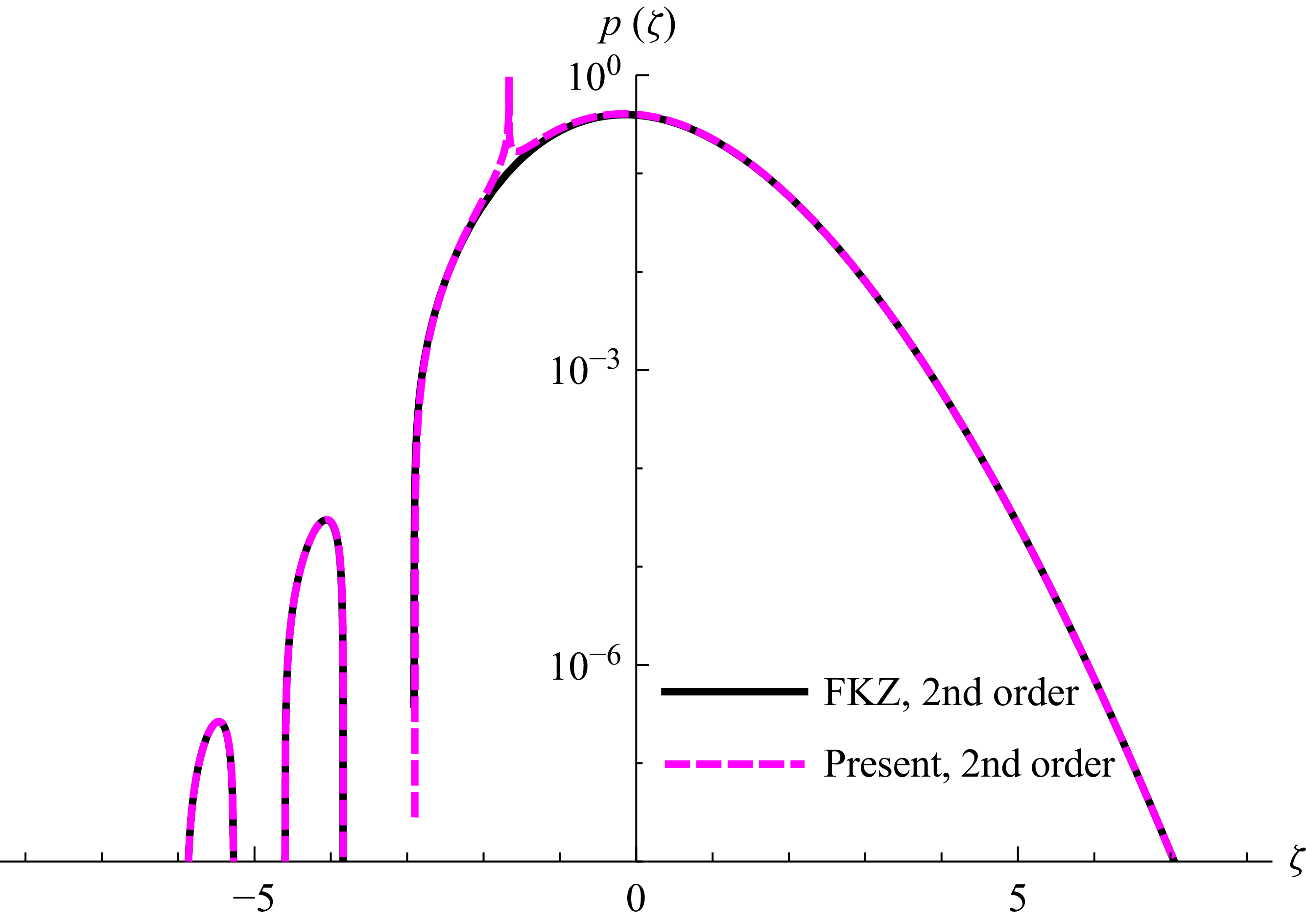
represents the complex conjugate. This approximation is compared with the second-order FKZ distribution (full line),
 $ {Ai}$
being the Airy function,
 \begin{equation} p(\zeta )=\left (\frac {2}{\kappa _3}\right )^{1/3} \exp \left (\frac {1}{3\kappa _3^2} + \frac {\zeta }{\kappa _3}\right ) \mbox{Ai}(\chi ), \quad \chi = \left (\frac {2}{\kappa _3}\right )^{1/3}\left (\frac {1}{2\kappa _3}+\zeta \right ), \end{equation}
in figure 2 for an example with
 $\kappa _3=0.3$
. Apart from the previously discussed singularity, the saddle-point approximation provides an excellent match with the full theoretical distribution. This is consistent with the rapid decay of
 ${\rm Re} (\phi (s))$
along the contours where
 ${\rm Im} (\phi (s))={\rm Im} (\phi (\tilde {s}))$
observed in figure 1, indicating that the approximation introduced via the Taylor series (2.5) should be very accurate.
Comparison of the second-order saddle-point approximation with the FKZ distribution, with
 $\kappa _3=0.3$
. Note the singularity occurring at
 $\zeta =\zeta _{crit}=-1/(2\kappa _3)=-1.\overline {6}$
.

3.3. Third order
When truncated at third order (3.2) incorporates both skewness and kurtosis:
 \begin{equation} \phi (s)=\mbox{i}\zeta s-\frac {s^2}{2} + \frac {\mbox{i}\kappa _3}{6} s^3 + \frac {\kappa _4}{24}s^4. \end{equation}
The saddle points now correspond to those where
 \begin{equation} \phi ^\prime (\tilde {s}) = \mbox{i}\zeta - \tilde {s} + \frac {\mbox{i}\kappa _3}{2}\tilde {s}^2 + \frac {\kappa _4}{6}\tilde {s}^3=0. \end{equation}
Being a third-order polynomial in
 $\tilde {s}$
, there are three saddle points, all of which are given by rather lengthy expressions.
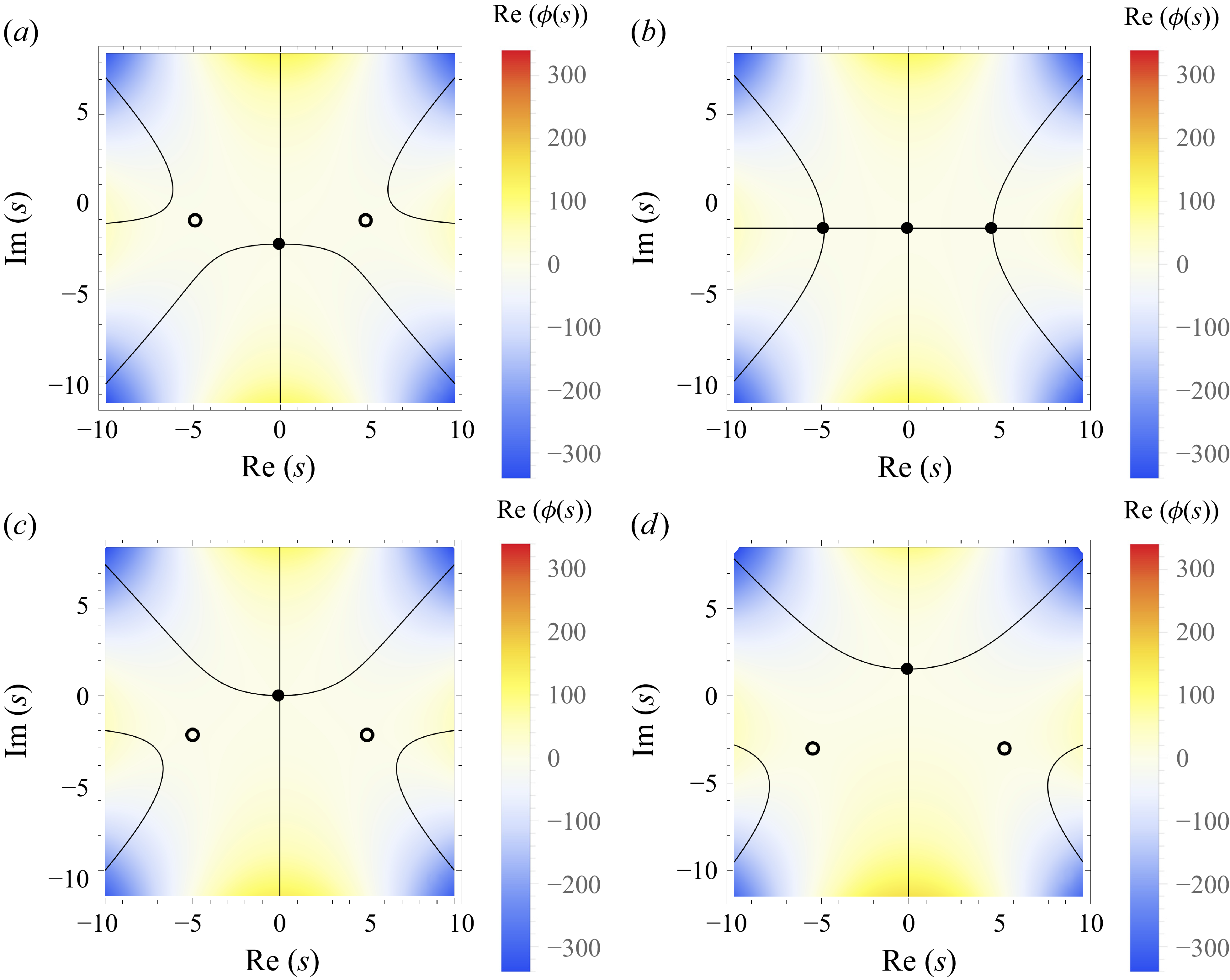
To determine which of these contribute, we will again perform an inspection of their positions in the complex plane. These are exemplified in figure 3 for cases with fixed
 $\kappa _3=0.3$
and
 $\kappa _4=0.2$
and variable
 $\zeta$
, in a fashion similar to that in figure 1. A critical point occurs at
 \begin{equation} \zeta _{crit}=\frac {\kappa _3^3-3\kappa _3\kappa _4}{3\kappa _4^2} \end{equation}
where all three saddle points lie on
 ${\rm Im} (\phi (s))=0$
contours (full lines), as depicted in figure 3(b). For
 $\zeta \gt \zeta _{crit}$
(figure 3
c,d), as well as
 $\zeta \lt \zeta _{crit}$
(figure 3
a), it is clear that there is a lone (purely imaginary) contributing saddle point, which lies directly on a
 ${\rm Im} (\phi (s))=0$
contour, which clearly represents the path of steepest descent. This structure implies that both positive and negative tails should be well behaved at third order. This is in stark contrast to the structurally inevitable oscillations in the negative tail observed at second order, which were explained through similar inspection of figure 1.
Plots showing the third-order saddle-point positions (black circles) in the complex plane, contours where
 ${\rm Im} (\phi (s))=0$
(full black lines) as well as
 ${\rm Re} (\phi (s))$
(colours). Results use fixed
 $\kappa _3=0.3$
and
 $\kappa _4=0.2$
with (
 $a$
)
 $\zeta =-2$
, (
 $b$
)
 $\zeta =\zeta _{crit}=-1.275$
from (3.16), (
 $c$
)
 $\zeta =0$
and (
 $d$
)
 $\zeta =2$
.

Since for
 $\zeta \neq \zeta _{crit}$
there is only a single contributing saddle point, we will utilise it to formulate an approximate PDF at third order. The (purely imaginary) saddle point, stemming from a solution to (3.15), may be written reasonably compactly as
 \begin{equation} \tilde {s}=\mbox{i}\gamma ,\end{equation}
where
 \begin{equation} \gamma = -\frac {1}{\kappa _4}\left ( \kappa _3 + \frac {\kappa _3^2-2\kappa _4}{\alpha ^{1/3}} + \alpha ^{1/3} \right ), \end{equation}
 \begin{equation} \alpha = \kappa _3^3 - 3\kappa _3\kappa _4 + \kappa _4(\sqrt {\beta } - 3\zeta \kappa _4), \end{equation}
 \begin{equation} \beta = -3\kappa _3^2\lambda + 2\kappa _4(4+9\zeta \kappa _3) + 9\zeta ^2\kappa _4^2 \end{equation}
and
 $\lambda$
is from (3.9). To arrive at the above it has been assumed that
 \begin{equation} \kappa _4\gt \frac {\kappa _3^2}{2}. \end{equation}
This condition likewise ensures that the cumulant generating function truncated at third order is convex for all real
 $s$
. The second derivative at the saddle point is
 \begin{equation} \phi ^{\prime \prime }(\tilde {s})=-1 - \gamma \kappa _3 - \frac {\gamma ^2\kappa _4}{2}. \end{equation}
Inserting all of the above into (2.6) finally leads to the third-order saddle-point approximation of the PDF:
 \begin{equation} p(\zeta ) \approx \tilde {p}(\zeta ) = \frac {1}{\sqrt {-2\pi \phi ^{\prime \prime }(\tilde {s})}} \exp \left (- \gamma \zeta + \frac {\gamma ^2}{2} + \frac {\gamma ^3\kappa _3}{6} + \frac {\gamma ^4\kappa _4}{24} \right ). \end{equation}
We will denote this approximation
 $\tilde {p}(\zeta )$
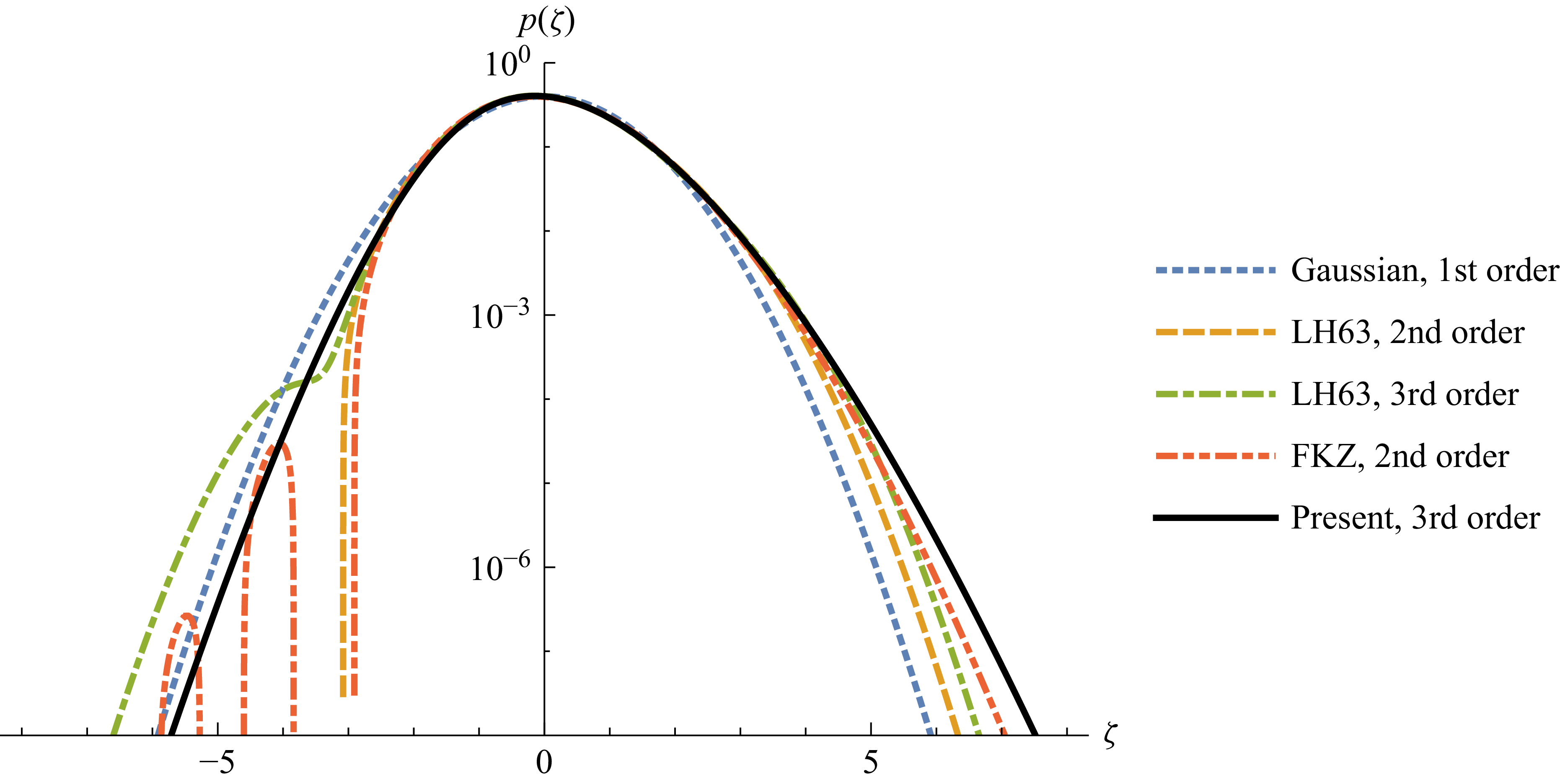
, as indicated above. This new result is compared with the Gaussian (first-order exact solution) distribution (3.5), those of LH63 (second- and third-order approximations) and FKZ (second-order exact solution) (3.13) in figure 4, for an example with
 $\kappa _3=0.3$
and
 $\kappa _4=0.2$
. It is seen that the present third-order saddle-point approximation has a heavier positive tail than all of these prior distributions, important, for example, in the prediction of large surface elevations typical of rogue waves. Moreover, apart from the Gaussian distribution, it is the only one of those shown to be free of unphysical oscillations in the negative tail. This behaviour is consistent with the expectations based on figure 3.
Comparison of the present third-order saddle-point approximation
 $\tilde {p}$
from (3.23), with the Gaussian (normal) distribution (3.5), the (second- and third-order) Gram–Charlier approximations of LH63 and the second-order FKZ distribution (3.13). All results use
 $\kappa _3=0.3$
and
 $\kappa _4=0.2$
.

4. Asymptotic analysis of the saddle-point approximations as
$\zeta \rightarrow \pm \infty$

4.1. First order
The first-order asymptotics are fully governed by the Gaussian distribution (3.5). From this, it is seen that both positive and negative tails decay with a term proportional to
 $\zeta ^2$
in the exponential function.
4.2. Second order
Let us now consider the asymptotics of the second-order saddle-point approximation from (3.12). In the positive-tail limit where
 $\zeta \rightarrow \infty$
this tends to
 \begin{equation} p(\zeta )\sim \frac {C}{\zeta ^{1/4}}\exp \left (a_1\zeta ^{3/2} + a_2\zeta + a_3\zeta ^{1/2} + a_4 + a_5\zeta ^{-1/2} + \cdots \right ). \end{equation}
For completeness we note that
 \begin{equation} a_1 = -\frac {2}{3}\left (\frac {2}{\kappa _3}\right )^{1/2}, \end{equation}
i.e. the dominant term in the exponential tail function is governed entirely by the skewness. The other
 $a_i$
coefficients can be inferred from (4.1) of FKZ, or alternatively are (up to
 $a_3$
) as provided in table 1 of Klahn et al. (Reference Klahn, Zhai and Fuhrman2024). The prefactor is
 \begin{equation} C = \frac {1}{2^{3/4}\sqrt {\pi }\kappa _3^{1/4}}. \end{equation}
The positive-tail asymptotics (4.1) from the saddle-point approximation thus coincide with those known from the second-order FKZ distribution (3.13). As emphasised by FKZ, with dominant term proportional to
 $\zeta ^{3/2}$
in the exponential function, the positive tail is fundamentally heavier than predicted by the Gaussian distribution (3.5), as well as both second- and third-order Gram–Charlier approximations of LH63, whose asymptotics are both similar to Gaussian (see § 4 of FKZ).
In the negative-tail limit
 $\zeta \rightarrow -\infty$
(3.12) tends to
 \begin{equation} p(\zeta )\sim \frac {1+\mbox{i}}{\sqrt {2}}\frac {C}{|\zeta |^{1/4}}\exp \left (\mbox{i}a_1|\zeta |^{3/2} + a_2|\zeta | + \mbox{i}a_3|\zeta |^{1/2} + a_4 + \mbox{i}a_5|\zeta |^{-1/2} + \cdots \right ) + \text{c.c.} \end{equation}
The (unphysical) oscillations in the negative tail are obviously due to the imaginary unit appearing in front of the
 $a_1$
,
 $a_3$
and
 $a_5$
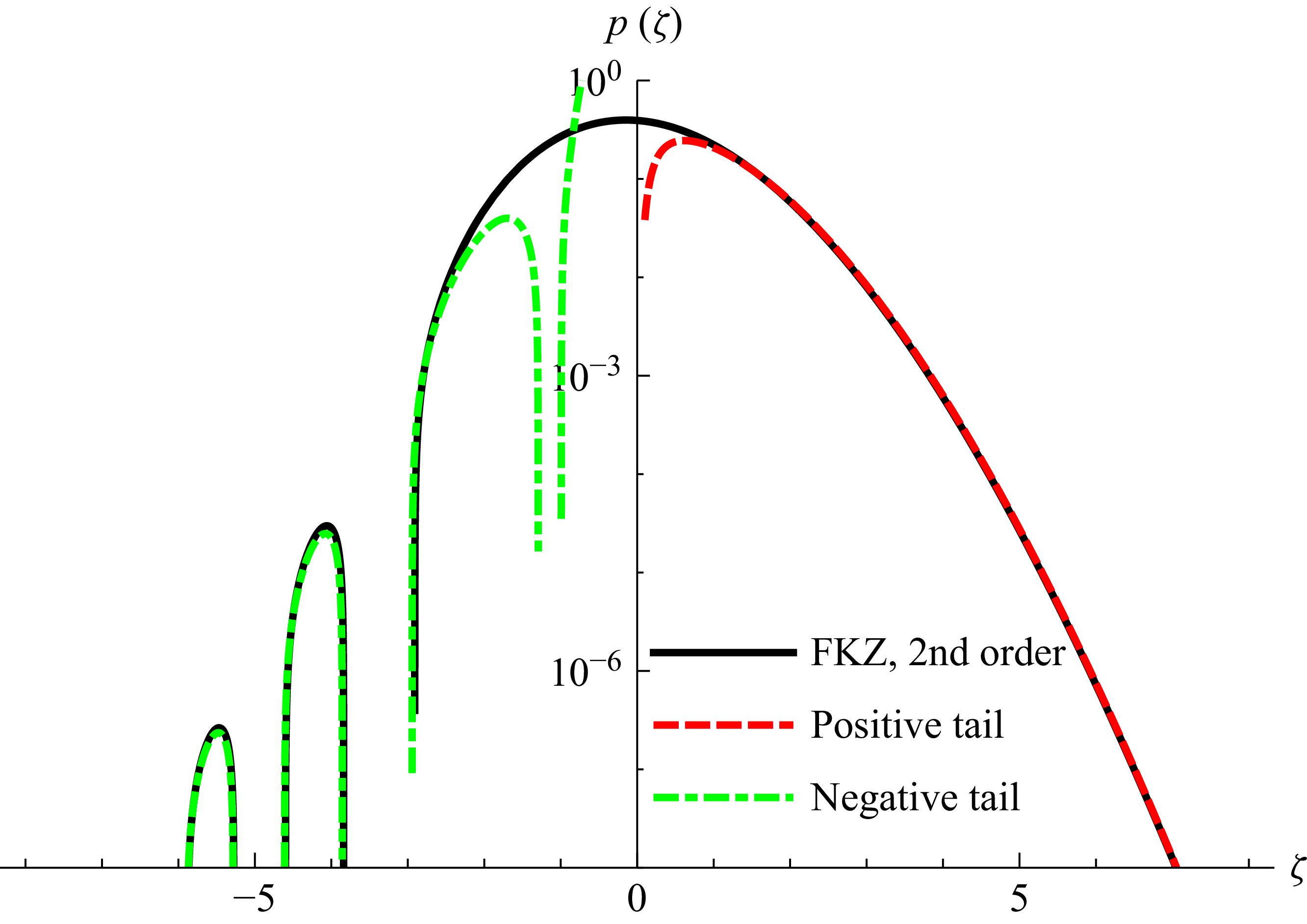
terms. Although this is the first time the second-order negative-tail asymptotics have been formally shown, these similarly match those of the FKZ distribution (3.13).
Comparison of these positive and negative tail asymptotics with the full second-order FKZ distribution is shown in figure 5, where an excellent match is indeed seen at both extrema. At second order, there are again no non-oscillatory solutions for the negative tail.
Comparison of the second-order FKZ distribution with the positive and negative asymptotic tail solutions with
 $\kappa _3=0.3$
.

4.3. Third order
We will now consider the tail asymptotics of the third-order saddle-point approximation
 $\tilde {p}(\zeta )$
from (3.23). In the positive-tail limit where
 $\zeta \rightarrow \infty$
(3.23) tends to
 \begin{equation} \tilde {p}(\zeta )\sim \frac {C}{\zeta ^{1/3}}\exp \left (a_1\zeta ^{4/3} + a_2\zeta + a_3\zeta ^{2/3} + a_4\zeta ^{1/3} + a_5 + a_6\zeta ^{-1/3} + a_7\zeta ^{-2/3} + \cdots \right ). \end{equation}
For completeness we note that
 \begin{equation} a_1 = -\frac {3}{2}\left (\frac {3}{4\kappa _4}\right )^{1/3}, \end{equation}
i.e. the dominant term in the exponential tail function is now governed entirely by the kurtosis. The other
 $a_i$
coefficients (up to
 $a_4$
) are as given in table 1 of Klahn et al. (Reference Klahn, Zhai and Fuhrman2024), with
 \begin{align} a_5=-\frac {3\kappa _3^4-12\kappa _3^2\kappa _4 + 8\kappa _4^2}{8\kappa _4^3}, \\[-28pt] \nonumber \end{align}
 \begin{align} a_6=\frac {\kappa _3^5-5\kappa _3^3\kappa _4+6\kappa _3\kappa _4^2}{3\times 6^{1/3}\kappa _4^{11/3}} \\[0pt] \nonumber \end{align}
and
 \begin{equation} a_7 = \frac {-7\kappa _3^6 + 42\kappa _3^4\kappa _4 - 72\kappa _3^2\kappa _4^2 + 24\kappa _4^3}{36\times 6^{2/3}\kappa _4^{13/3}}. \end{equation}
The (previously unknown) prefactor is
 \begin{equation} C = \frac {1}{6^{1/3}\sqrt {\pi }\kappa _4^{1/6}}. \end{equation}
The asymptotic form (4.5) stemming from the saddle-point approximation (3.23) reproduces the exact exponential scaling obtained previously via the method of dominant balance by Klahn et al. (Reference Klahn, Zhai and Fuhrman2024). Analysis of the saddle-point approximation additionally yields the prefactor
 $C$
, thereby newly providing the full formal asymptotic expression, accounting for both skewness and kurtosis. Determination of
 $a_5$
,
 $a_6$
and
 $a_7$
above is likewise new. As emphasised by Klahn et al. (Reference Klahn, Zhai and Fuhrman2024), with dominant term proportional to
 $\zeta ^{4/3}$
in the exponential function, the positive third-order tail is fundamentally even heavier than at second order, consistent with what is shown in figure 4.
In the negative-tail limit where
 $\zeta \rightarrow -\infty$
(3.23) tends to
 \begin{equation} \tilde {p}(\zeta )\sim \frac {C}{|\zeta |^{1/3}}\exp \left (a_1|\zeta |^{4/3} - a_2|\zeta | + a_3|\zeta |^{2/3} - a_4|\zeta |^{1/3} + a_5 - a_6|\zeta |^{-1/3} + a_7|\zeta |^{-2/3} + \cdots \right ). \end{equation}
This result is entirely new. Interestingly, the theoretical negative tail is formally just as heavy as the positive tail, with dominant term proportional to
 $|\zeta |^{4/3}$
in the exponential. The more rapid decay in the negative, relative to the positive, tail in practice is due to the sign reversal on the subdominant
 $a_2$
,
 $a_4$
and
 $a_6$
terms.
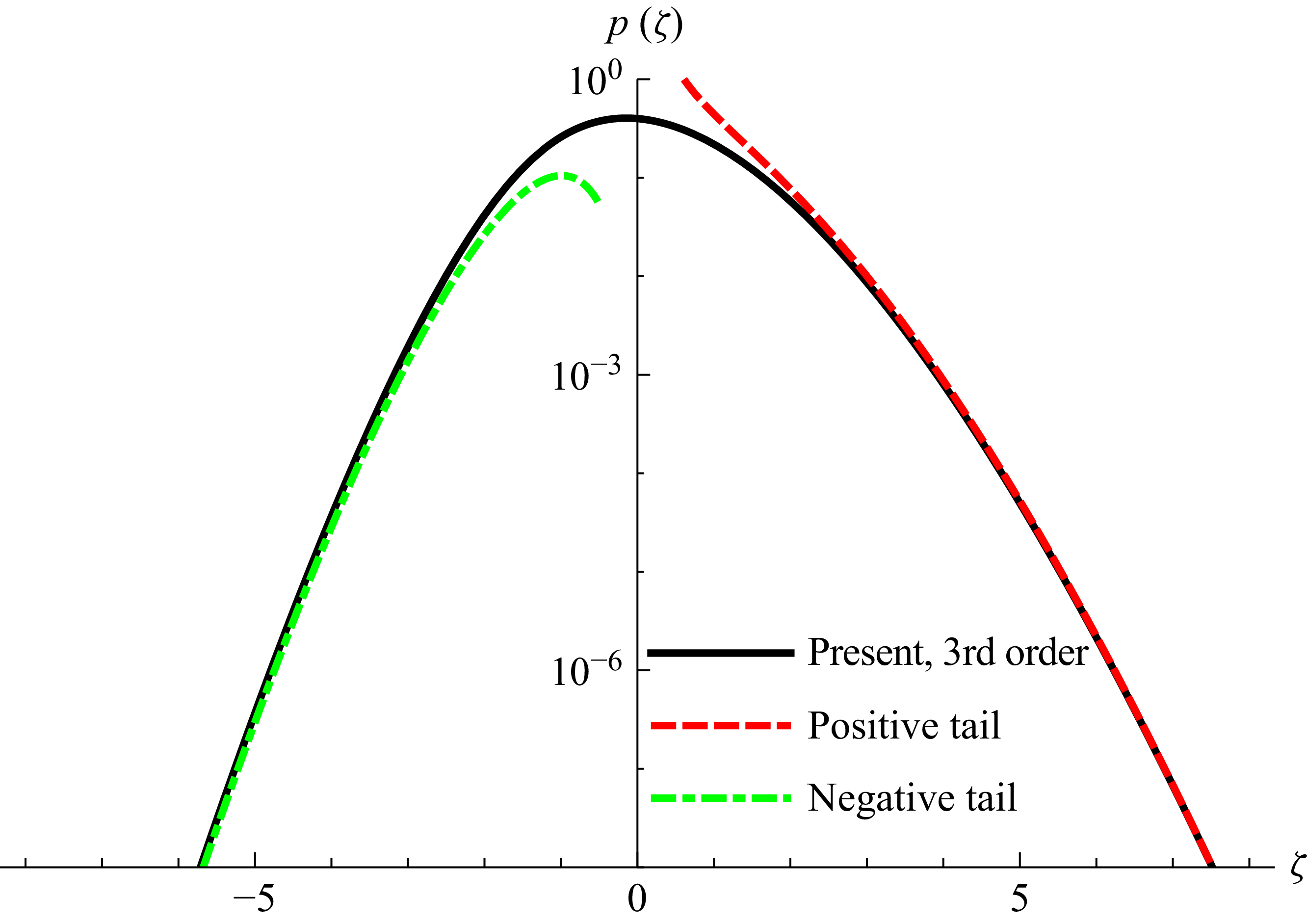
Comparison of both positive- and negative-tail asymptotics with the third-order saddle-point approximation (3.23) is provided in figure 6 for a case with
 $\kappa _3=0.3$
and
 $\kappa _4=0.2$
, where an excellent match is again observed. In contrast to the second-order solution, the third-order saddle-point approximation clearly yields a negative tail free of unphysical oscillations, as discussed previously. This thus resolves a problem common to both second- and third-order approximations of LH63, the exact second-order FKZ distribution (3.13) as well as the third- and higher-order numerical solutions obtained by Klahn et al. (Reference Klahn, Zhai and Fuhrman2024) and Zhai et al. (Reference Zhai, Klahn, Onorato and Fuhrman2025).
Comparison of the third-order tail asymptotics with the saddle-point approximation
 $\tilde {p}(\zeta )$
from (3.23), with
 $\kappa _3=0.3$
and
 $\kappa _4=0.2$
.

4.4. Higher orders
A novel perturbation method is developed in Appendix A, which is utilised to derive the positive- and negative-tail asymptotics at fourth and fifth orders. These are again generally in line with the form arrived at by Klahn et al. (Reference Klahn, Zhai and Fuhrman2024), with the previously unknown prefactors again newly determined. Similar to second order, the fourth-order negative tail is oscillatory. Similar to third order, at fifth order a non-oscillatory, decaying solution for the negative tail is found. Hence, it seems that unphysical, oscillatory negative tails are structural artefacts common to the LH63 integral truncated at even orders, which can be remedied by going to the next odd order.
5. Analysis of the third-order saddle-point approximation
$\tilde {p}(\zeta )$

Of the results found above, the one of principal novel interest is the third-order saddle-point approximation,
 $\tilde {p}(\zeta )$
, given in (3.23). We will therefore analyse its accuracy in terms of integrated statistical properties in the present section, first in raw form (un-normalised) and then in a normalised form.
5.1. Un-normalised
To analyse the accuracy of
 $\tilde {p}(\zeta )$
from (3.23), we will consider its fundamental integral
 \begin{equation} \tilde {\mathcal{I}} = \int _{-\infty }^\infty \tilde {p}(\zeta )\, \mbox{d}\zeta , \end{equation}
which should, of course, ideally give unity. We will additionally consider the mean (assumed zero)
 \begin{equation} \tilde {\mu }=\int _{-\infty }^\infty \zeta \tilde {p}(\zeta )\, \mbox{d}\zeta , \end{equation}
variance (assumed to be unity)
 \begin{equation} \tilde {\sigma }^2=\int _{-\infty }^\infty \zeta ^2 \tilde {p}(\zeta )\, \mbox{d}\zeta , \end{equation}
as well as its skewness (in principle, input as
 $\kappa _3$
)
 \begin{equation} \tilde {\mathcal{S}}=\int _{-\infty }^\infty \zeta ^3 \tilde {p}(\zeta )\, \mbox{d}\zeta \end{equation}
and excess kurtosis
 $\tilde {\mathcal{K}}-3$
(in principle, input as
 $\kappa _4$
), where
 \begin{equation} \tilde {\mathcal{K}}=\int _{-\infty }^\infty \zeta ^4 \tilde {p}(\zeta )\, \mbox{d}\zeta . \end{equation}
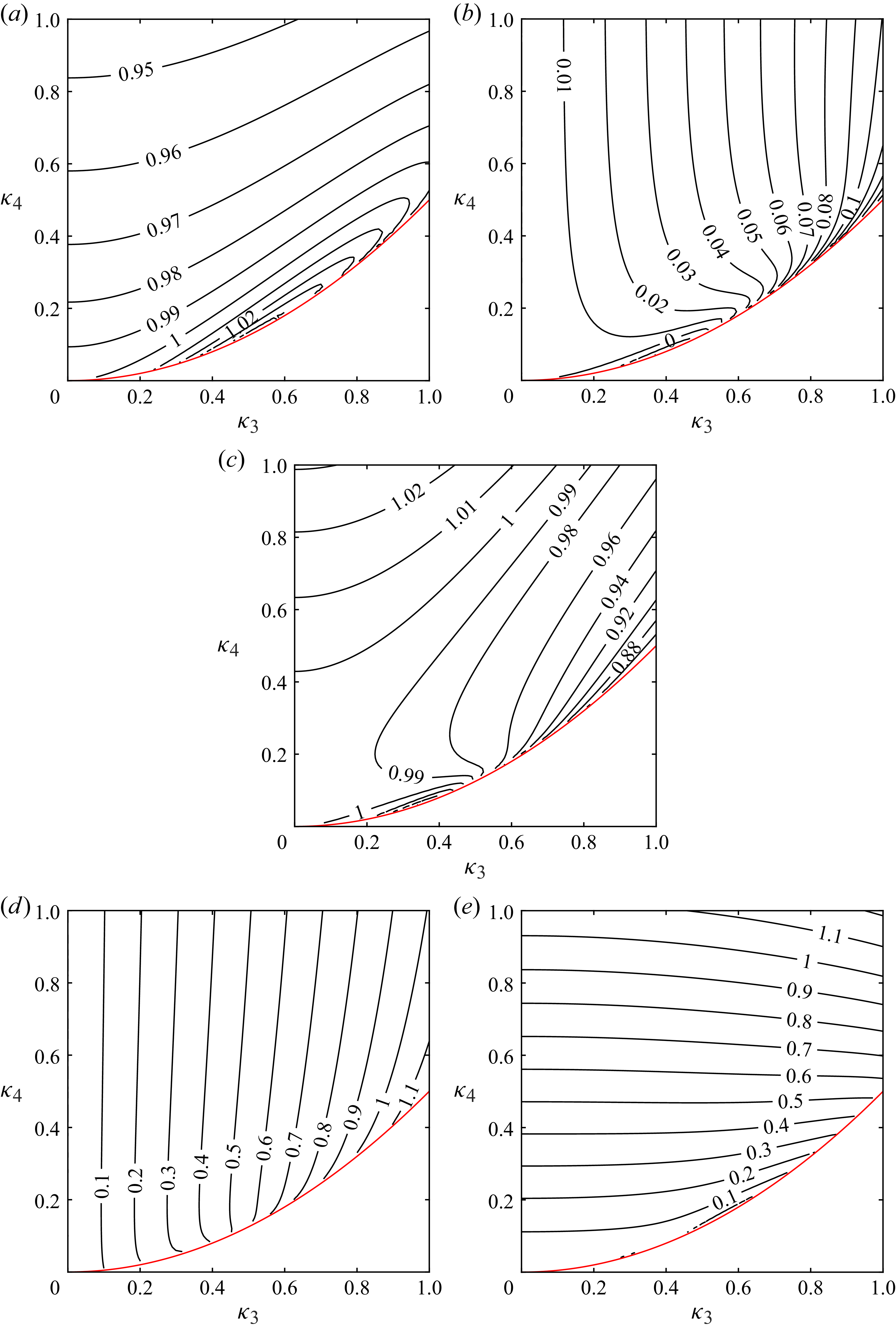
Contour plots depicting the variation of (
 $a$
)
 $\tilde {\mathcal{I}}$
, (
 $b$
)
 $\tilde {\mu }$
, (
 $c$
)
 $\tilde {\sigma }^2$
, (
 $d$
)
 $\tilde {\mathcal{S}}$
and (
 $e$
)
 $\tilde {\mathcal{K}}-3$
for input
 $\kappa _3$
and
 $\kappa _4$
based on the third-order saddle-point approximation
 $\tilde {p}(\zeta )$
from (3.23). Note that the red lines correspond to
 $\kappa _4=\kappa _3^2/2$
, below which
 $\tilde {p}(\zeta )$
becomes complex.

Contour plots for each of these quantities are provided in figure 7. Because
 $\tilde {p}(\zeta )$
from (3.23) is only an approximation of
 $p(\zeta )$
at third order, it is seen that each of the integrated quantities above do not result in exactly the idealised values. They are, however, reasonably close, especially for moderate
 $\kappa _3$
and
 $\kappa _4$
. The contours for
 $\tilde {\mathcal{S}}$
and
 $\tilde {\mathcal{K}}-3$
are, respectively, nearly vertical and horizontal in figures 7(d) and 7(e), such that (3.23) gives quite a reasonable first approximation. Note that in the uncontoured region in the lower right of each subfigure in figure 7, (3.23) yields complex numbers, and cannot be used. This region corresponds to where assumption (3.21) is violated, and this threshold is indicated by the red lines (similarly in forthcoming figures 8–10).
5.2. Normalised
A proper PDF can be formed from
 $\tilde {p}(\zeta )$
via the following normalisation:
 \begin{equation} p(\zeta ) = \frac {\hat {\sigma }}{\tilde {\mathcal{I}}}\tilde {p}(\hat {\sigma }\zeta +\hat {\mu }), \end{equation}
where
 \begin{equation} \hat {\mu }=\frac {1}{\tilde {\mathcal{I}}}\int _{-\infty }^\infty \zeta \tilde {p}(\zeta )\,\mbox{d}\zeta \end{equation}
and
 \begin{equation} \hat {\sigma }^2=\frac {1}{\tilde {\mathcal{I}}}\int _{-\infty }^\infty (\zeta -\hat {\mu })^2\tilde {p}(\zeta )\,\mbox{d}\zeta . \end{equation}


This normalisation shifts
 $\kappa _1$
and scales
 $\kappa _2$
relative to their raw values in the original truncated cumulant generating function. It is here motivated by pragmatism, as it is required to enforce a proper PDF,
 $p(\zeta )$
, having
 \begin{equation} \mathcal{I}=\int _{-\infty }^\infty p(\zeta )\,\mbox{d}\zeta =1, \end{equation}
 \begin{equation} \mu =\int _{-\infty }^\infty \zeta p(\zeta )\,\mbox{d}\zeta =0 \end{equation}
and
 \begin{equation} \sigma ^2=\int _{-\infty }^\infty \zeta ^2p(\zeta )\,\mbox{d}\zeta =1, \end{equation}
i.e. unit integral, zero mean and unit variance, fully consistent with the true statistical properties of
 $\zeta$
.
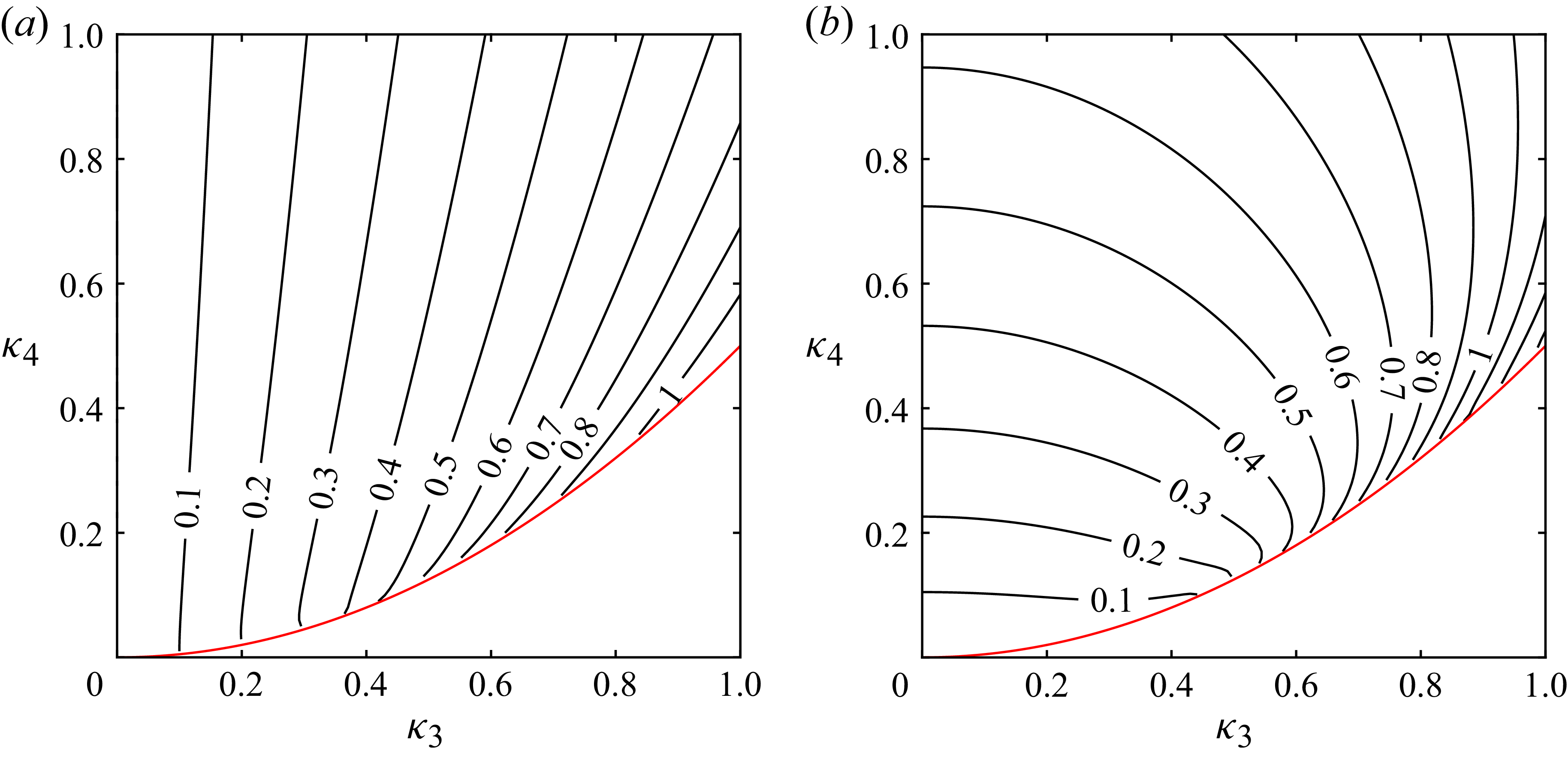
Contour plots depicting the resulting integral skewness
 \begin{equation} \mathcal{S}=\int _{-\infty }^\infty \zeta ^3p(\zeta )\,\mbox{d}\zeta \end{equation}
and excess kurtosis
 $\mathcal{K}-3$
, where
 \begin{equation} \mathcal{K}=\int _{-\infty }^\infty \zeta ^4p(\zeta )\,\mbox{d}\zeta , \end{equation}
for various input
 $\kappa _3$
and
 $\kappa _4$
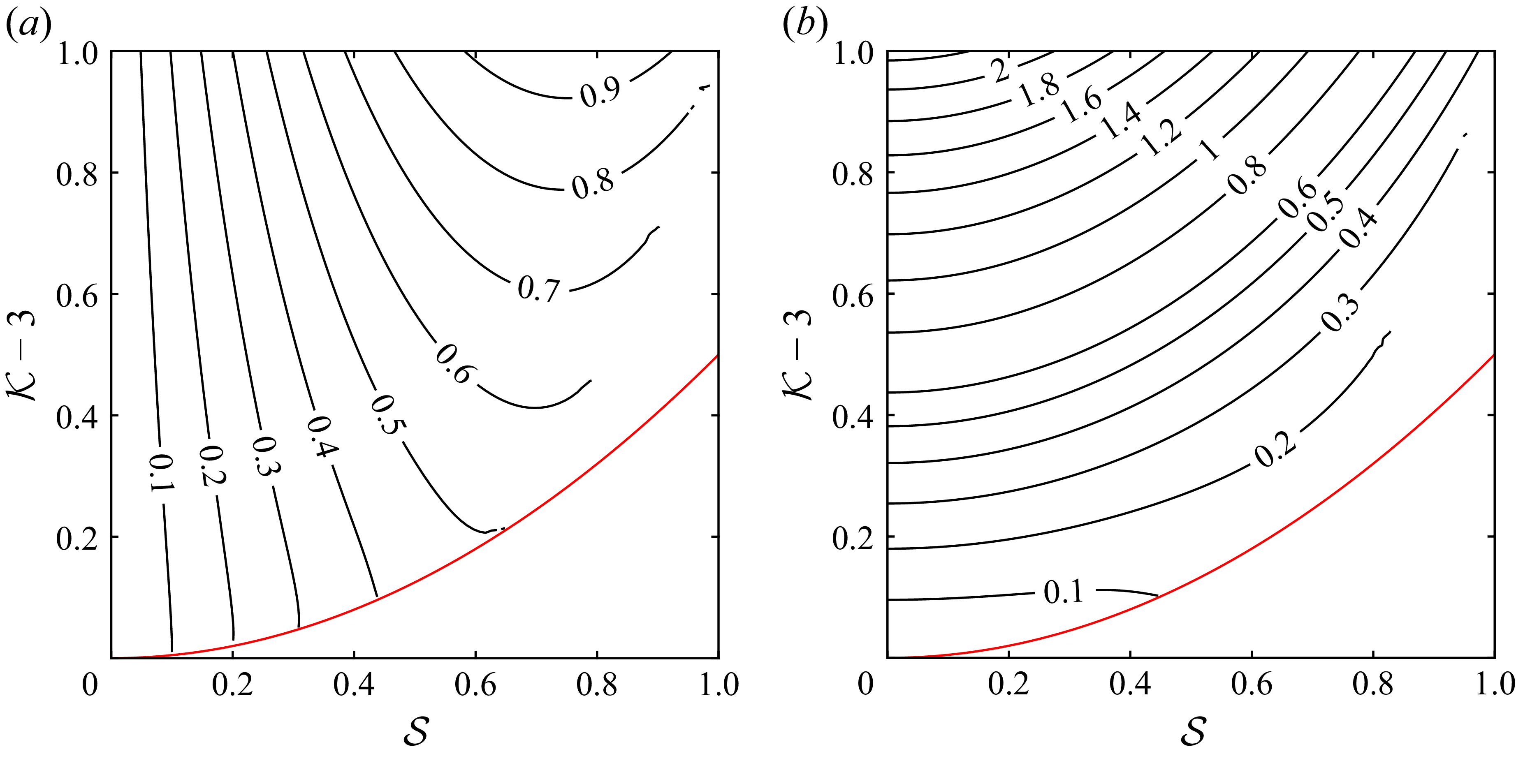
are provided in figure 8. Since the first two cumulants are already manipulated to enforce zero mean and unit variance, it is natural to treat the third and fourth cumulants with similar freedom. Inspection of figure 8 shows that the input cumulants
 $\kappa _3$
and
 $\kappa _4$
can likewise be adjusted (typically slightly, especially for moderate values) to yield PDFs matching desired skewness and kurtosis combinations in practice. The adjusted inputs thus correspond to the
 $(\kappa _3,\kappa _4)$
coordinates at the intersection of the desired
 $\mathcal{S}$
and
 $\mathcal{K}-3$
contours in figure 8. Finding these is easily automated using a root-finding function, which has been used to produce the inverse of figure 8 presented in figure 9, i.e. contour plots for
 $\kappa _3$
and
 $\kappa _4$
required to yield a prescribed
 $\mathcal{S}$
and
 $\mathcal{K}-3$
combination. This procedure essentially involves simultaneous iterative solution of (5.12) and (5.13) (with integrals evaluated numerically) to determine the required
 $(\kappa _3,\kappa _4)$
combination, using
 $(\mathcal{S},\mathcal{K}-3)$
as initial guesses. It is emphasised that the resulting tail behaviour in such normalised PDFs will be governed by the adjusted
 $\kappa _3$
and
 $\kappa _4$
values.
Contour plots depicting the variation of input cumulants (
 $a$
)
 $\kappa _3$
and (
 $b$
)
 $\kappa _4$
required to yield a desired combination of
 $\mathcal{S}$
and
 $\mathcal{K}-3$
using the normalised PDF
 $p(\zeta )$
from (5.6). The red lines correspond to
 $\mathcal{K}-3=\mathcal{S}^2/2$
, the lower bound based on (3.21).


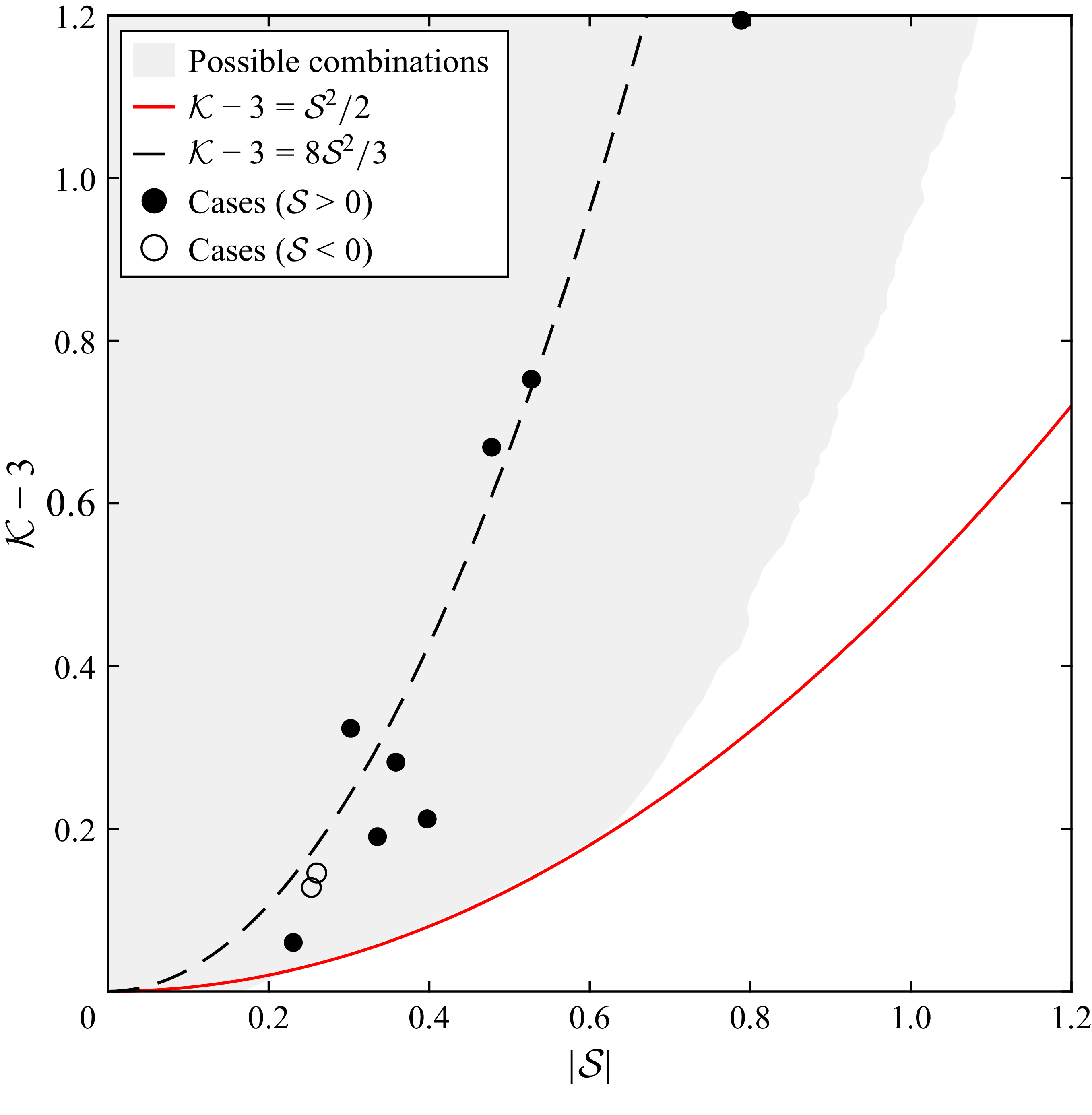
The possible parameter space in terms of
 $|\mathcal{S}|$
and
 $\mathcal{K}-3$
combinations is presented as the shaded region in figure 10, there extending up to 1.2 on both axes. (Note that the possible space is symmetric about
 $\mathcal{S}=0$
, i.e. solutions admit both positive and negative skewness, and hence
 $|\mathcal{S}|$
is used on the abscissa.) As seen there, as well as from the contoured regions in figure 9, the possible parameter space essentially corresponds to
 \begin{equation} \mathcal{K}-3 \gt \frac {\mathcal{S}^2}{2}, \end{equation}
with this threshold presented as the full red line, for
 $|\mathcal{S}|\lt 0.6$
, consistent with the assumption (3.21). For
 $|\mathcal{S}|\gt 0.6$
the possible space is more restrictive, as is evident from figure 10. Also shown as a reference in figure 10 (dashed black line) is the relation implied by Socquet-Juglard et al. (Reference Socquet-Juglard, Dysthe, Trulsen, Krogstad and Liu2005):
 \begin{equation} \mathcal{K}-3 = \frac {8\mathcal{S}^2}{3}, \end{equation}
for uni-directional, narrow-banded, deep-water wave fields, as well as the test cases to be considered in § 6 (
 $\mathcal{S}\gt 0$
: filled circles,
 $\mathcal{S}\lt 0$
: open circles), which loosely follow this trend. This reference line thus serves as a rough indication of
 $\mathcal{S}$
and
 $\mathcal{K}-3$
combinations likely to be encountered in practice, as skewness and kurtosis are not independent in irregular seas.
Normalised PDFs, as described above, will be presented exclusively in what follows, ensuring that all third-order PDFs shown have (numerically) integrated statistics (
 $\mathcal{I}=1$
,
 $\mu =0$
,
 $\sigma ^2=1$
, prescribed
 $\mathcal{S}$
and
 $\mathcal{K}$
) matching those of
 $\zeta$
from the various datasets against which they are compared in the next section.
6. Results
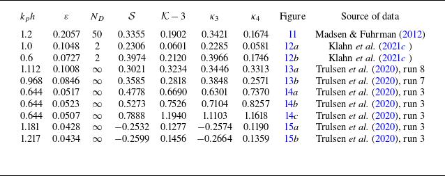
We will now test the accuracy of the new (normalised) third-order PDF from (5.6) by comparing against irregular wave datasets generated analytically, numerically and experimentally. All cases considered throughout the present section are summarised in table 1. The summary includes the input
 $\kappa _3$
and
 $\kappa _4$
values required to yield the exact
 $\mathcal{S}$
and
 $\mathcal{K}$
for each case considered. These combinations are again presented in figure 10 as the circles. All cases utilise a bin size of
 $\Delta \zeta =0.2$
. Error bars are likewise included, estimated as
 $\pm p(\zeta )/\sqrt {N_b}$
, where
 $N_b$
is the number of samples in each bin, following Onorato et al. (Reference Onorato2009). Throughout the present section we focus on challenging cases with
 $|\mathcal{S}|\gt 0.2$
, where the second-order FKZ distribution fails to provide sufficient accuracy, even in the well-behaved positive tail.
Summary of cases considered in the present work. Note that the listed
 $\kappa _3$
and
 $\kappa _4$
values correspond to the inputs required to yield
 $p(\zeta )$
from (5.6) having the listed skewness
 $\mathcal{S}$
and excess kurtosis
 $\mathcal{K}-3$
. All PDFs shown in the referenced figures have
 $\mathcal{I}=1$
,
 $\mu =0$
and
 $\sigma ^2=1$
. Variable
 $N_D$
is the directional spreading parameter, with
 $N_D=\infty$
indicating a uni-directional wave field.

Table 1. Long description
A table summarizing cases considered in a study on wave datasets. The table has 10 rows and 9 columns. Column headers are k p h, ε, N D, S, K - 3, κ 3, κ 4, Figure, and Source of data. Row 1: k p h, 1.2; ε, 0.2057; N D, 50; S, 0.3355; K - 3, 0.1902; κ 3, 0.3421; κ 4, 0.1674; Figure, 11; Source of data, Madsen & Fuhrman (2012). Row 2: k p h, 1.0; ε, 0.1048; N D, 2; S, 0.2306; K - 3, 0.0601; κ 3, 0.2285; κ 4, 0.0581; Figure, 12a; Source of data, Klahn et al. (2021c). Row 3: k p h, 0.6; ε, 0.0727; N D, 2; S, 0.3974; K - 3, 0.2120; κ 3, 0.3966; κ 4, 0.1746; Figure, 12b; Source of data, Klahn et al. (2021c). Row 4: k p h, 1.112; ε, 0.1008; N D, ∞; S, 0.3021; K - 3, 0.3234; κ 3, 0.3446; κ 4, 0.3313; Figure, 13a; Source of data, Trulsen et al. (2020), run 8. Row 5: k p h, 0.968; ε, 0.0846; N D, ∞; S, 0.3585; K - 3, 0.2818; κ 3, 0.3848; κ 4, 0.2571; Figure, 13b; Source of data, Trulsen et al. (2020), run 7. Row 6: k p h, 0.644; ε, 0.0517; N D, ∞; S, 0.4778; K - 3, 0.6690; κ 3, 0.6301; κ 4, 0.7370; Figure, 14a; Source of data, Trulsen et al. (2020), run 3. Row 7: k p h, 0.644; ε, 0.0523; N D, ∞; S, 0.5273; K - 3, 0.7526; κ 3, 0.7104; κ 4, 0.8257; Figure, 14b; Source of data, Trulsen et al. (2020), run 3. Row 8: k p h, 0.644; ε, 0.0507; N D, ∞; S, 0.7888; K - 3, 1.1940; κ 3, 1.1103; κ 4, 1.1618; Figure, 14c; Source of data, Trulsen et al. (2020), run 3. Row 9: k p h, 1.181; ε, 0.0428; N D, ∞; S, -0.2532; K - 3, 0.1277; κ 3, -0.2574; κ 4, 0.1190; Figure, 15a; Source of data, Trulsen et al. (2020), run 3. Row 10: k p h, 1.217; ε, 0.0434; N D, ∞; S, -0.2599; K - 3, 0.1456; κ 3, -0.2664; κ 4, 0.1359; Figure, 15b; Source of data, Trulsen et al. (2020), run 3.
The present third-order PDF requires both skewness and kurtosis to be known, or reasonably estimated, for practical use. While we utilise the values computed directly from sample data in the comparisons that follow, it can be noted that Gramstad & Lian (Reference Gramstad and Lian2024) have recently provided an empirical method for estimating both skewness and kurtosis for a given characteristic wave steepness, dimensionless water depth, directional spreading and frequency bandwidth, which was shown to be valid over a wide range of sea states. The present third-order PDF may be utilised in combination with their estimates in practice where sea state characteristics, but not necessarily the surface elevation statistics, are known or can be approximated.
6.1. Comparison with second-order irregular wave theory
To test the new third-order PDF, we will start by comparing against one based on data synthetically generated utilising the irregular wave theory of Madsen & Fuhrman (Reference Madsen and Fuhrman2012) carried out to second order. We will consider a case first considered by FKZ in their figure 9(c). This case is based on a wave field generated from a JONSWAP spectrum on finite depth
 $k_ph=1.2$
with steepness
 $\varepsilon =k_pH_{m0}/2=2k_p\sigma _\eta =0.2057$
, where
 $k_p$
is the peak wavenumber and
 $H_{m0}$
is the spectral significant wave height, with directional spreading parameter
 $N_D=50$
. For further details on this case, see § 6.1 of FKZ. This case results in a nonlinear, directionally spread, irregular wave field with skewness
 $\mathcal{S}=0.3355$
and kurtosis
 $\mathcal{K}=3.1902$
.
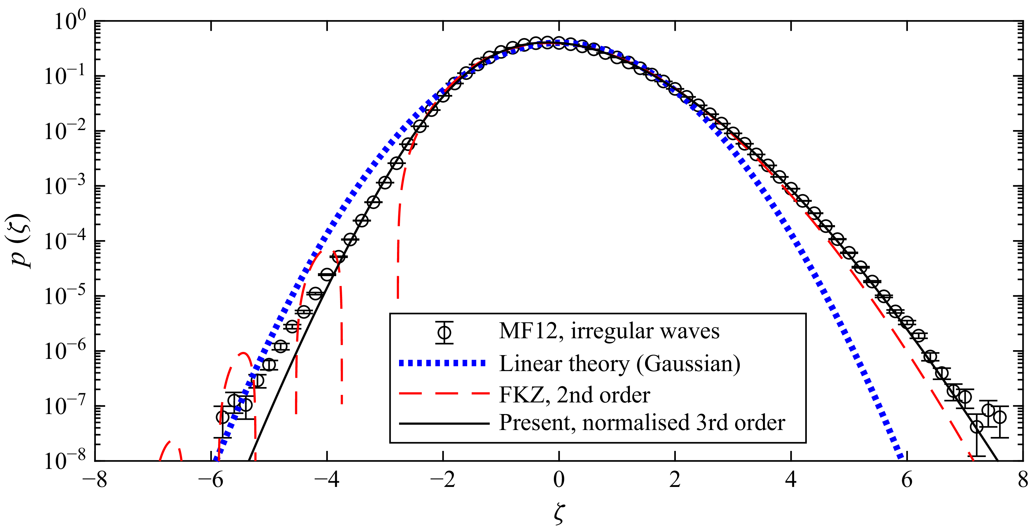
The resulting PDF from this dataset is presented in figure 11 as the open circles. Also shown are the (first-order) Gaussian distribution from (3.5), the second-order FKZ distribution (3.13) and the present third-order (normalised) saddle-point approximation (5.6). As seen, this dataset is clearly non-Gaussian. The present third-order distribution provides an excellent match with the data, especially in the heavy positive tail. Unlike the second-order FKZ distribution, or the third-order numerical result of Klahn et al. (Reference Klahn, Zhai and Fuhrman2024) (see their figure 2), the present third-order distribution again avoids unphysical oscillations in the negative tail, where the match with the data is good for
 $\zeta \gt -4$
; for
 $\zeta \lt -4$
deviations are apparent.
Comparison with data generated from the second-order irregular wave theory of Madsen & Fuhrman (Reference Madsen and Fuhrman2012), cited as MF12 in the legend. This case considers
 $\mathcal{S}=0.3355$
and
 $\mathcal{K}=3.1902$
.

6.2. Comparison with fully nonlinear wave model results
As a second means of comparison, we will compare with directionally spread wave fields generated by the fully nonlinear numerical model of Klahn et al. (Reference Klahn, Madsen and Fuhrman2021c ). This model utilises an artificial lower boundary condition of Nicholls (Reference Nicholls2011) and makes use of a linearised preconditioner, following Fuhrman & Bingham (Reference Fuhrman and Bingham2004). For validation and prior applications of this model, see e.g. Klahn et al. (Reference Klahn, Madsen and Fuhrman2021a ,Reference Klahn, Madsen and Fuhrman b ) and Zhai et al. (Reference Zhai, Klahn, Onorato and Fuhrman2025).
Two cases will be considered. The first is from a dataset originally considered by FKZ, with
 $k_ph=1$
and
 $\varepsilon =0.1048$
(having
 $\mathcal{S}=0.2306$
and
 $\mathcal{K}=3.0601$
). The second is from a dataset originally considered by Klahn et al. (Reference Klahn, Zhai and Fuhrman2024), with
 $k_ph=0.6$
and
 $\varepsilon =0.0727$
(having
 $\mathcal{S}=0.3974$
and
 $\mathcal{K}=3.2120$
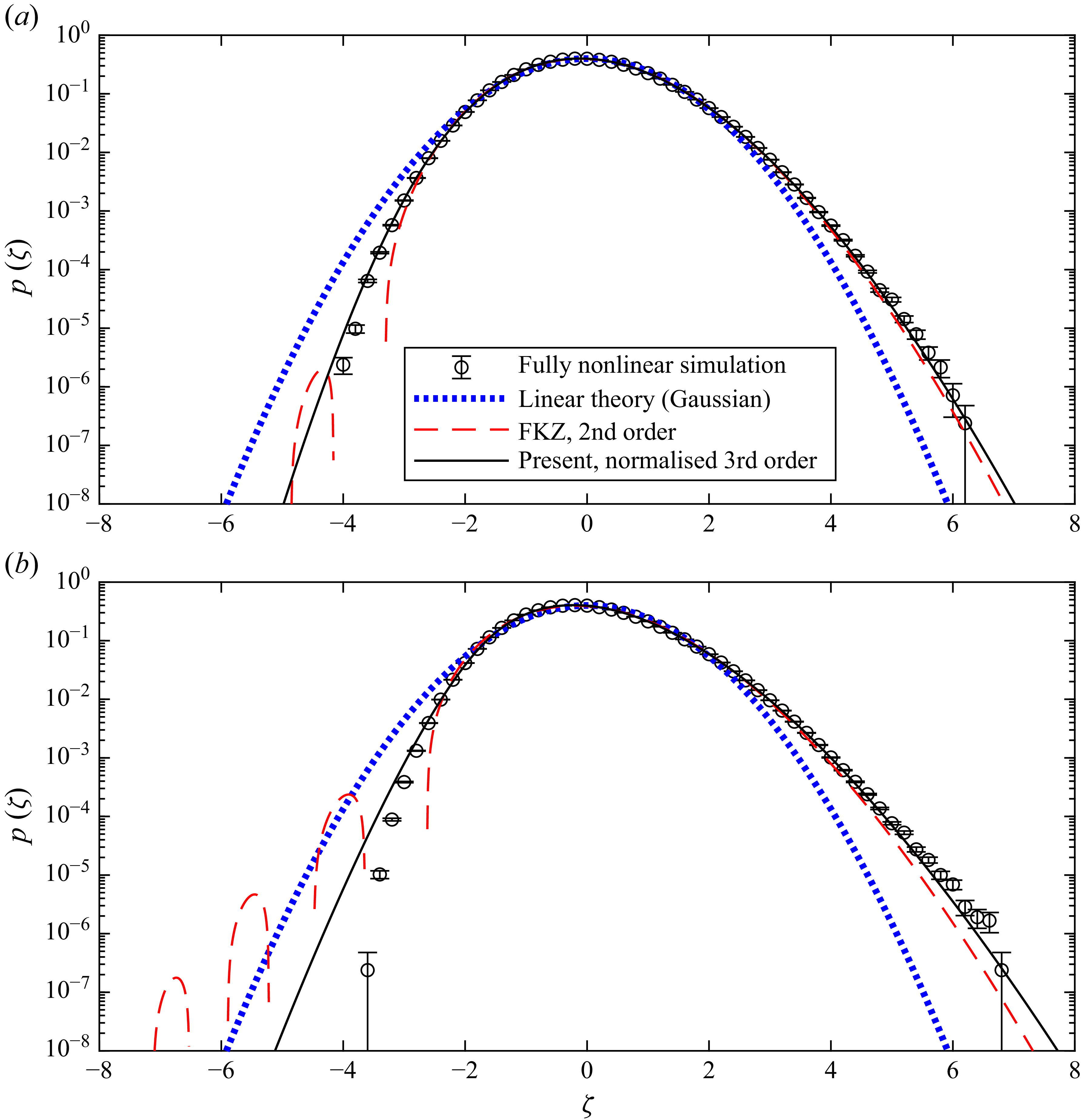
). Results can been seen in figure 12. For the case with
 $\mathcal{S}=0.2306$
and
 $\mathcal{K}=3.0601$
(figure 12
a) the match is excellent over nearly the entire range covered by the data. For the case with
 $\mathcal{S}=0.3974$
and
 $\mathcal{K}=3.2120$
(figure 12
b) the match is acceptable, though the positive tail is slightly underestimated by the new third-order theory, with the negative tail being overestimated.
Comparison with datasets generated from fully nonlinear wave model (Klahn et al. Reference Klahn, Madsen and Fuhrman2021c
) simulations with (a)
 $\mathcal{S}=0.2306$
,
 $\mathcal{K}=3.0601$
and (b)
 $\mathcal{S}=0.3974$
,
 $\mathcal{K}=3.2120$
.

6.3. Comparison with irregular wave experiments
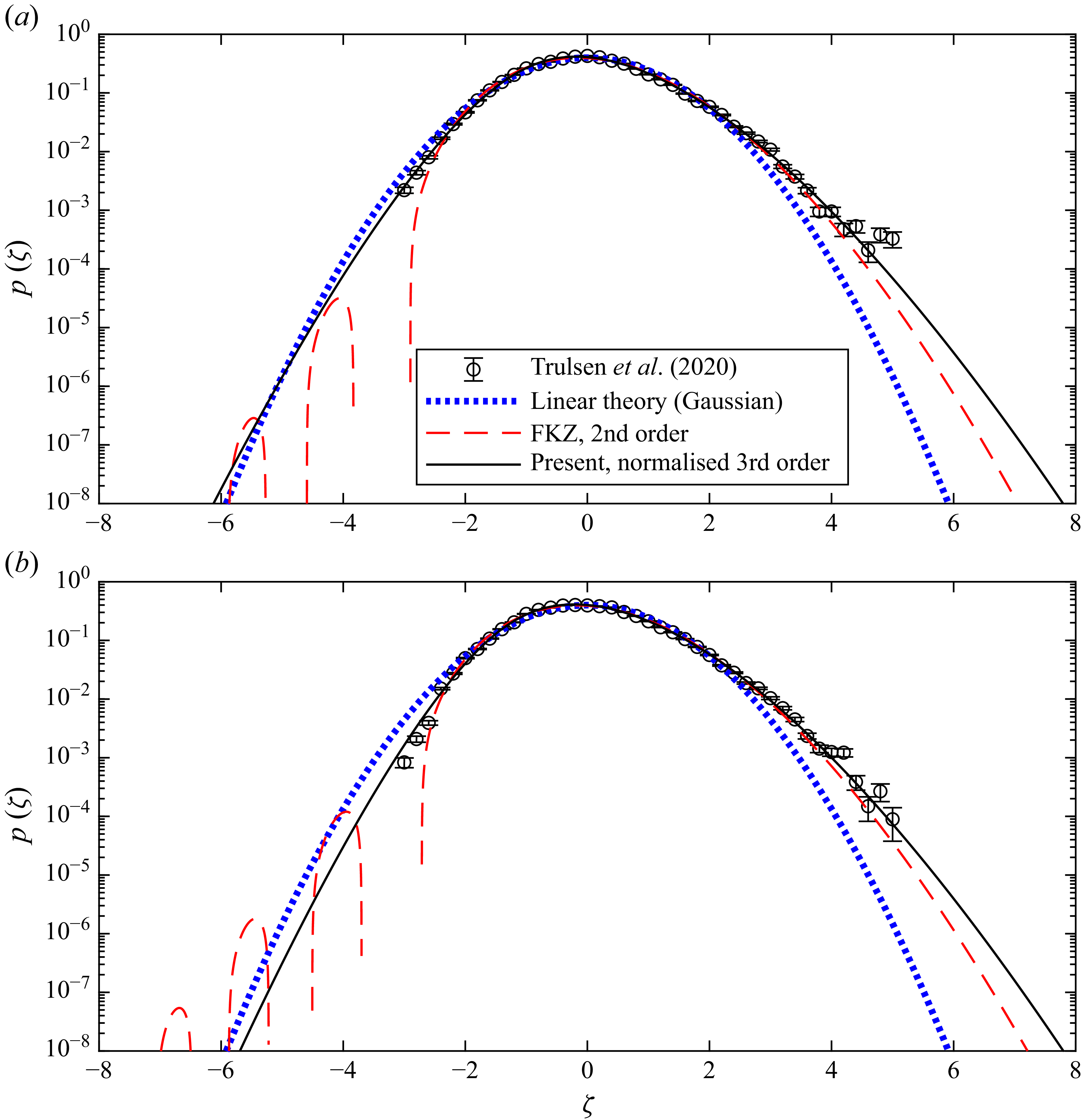
We will finally consider numerous cases from the dataset of Trulsen et al. (Reference Trulsen, Raustol, Jorde and Rye2020), who performed experiments involving uni-directional irregular wave fields propagating over a shoal. Comparisons with selected cases having moderate skewness
 $\mathcal{S}\gt 0$
from their runs 7 and 8 are first presented in figure 13. The first case, presented in figure 13(a), has
 $\mathcal{S}=0.3021$
and
 $\mathcal{K}=3.3234$
. The present new third-order result matches the data (both positive and negative tails) quite convincingly. The second case considered has
 $\mathcal{S}=0.3585$
and
 $\mathcal{K}=3.2818$
and is presented in figure 13(b). In this case the positive tail is captured with high accuracy, though the negative tail is slightly overestimated.
Comparison with selected datasets from Trulsen et al. (Reference Trulsen, Raustol, Jorde and Rye2020): (a) run 8 at their horizontal position
 $x$
= 1.9 m (
 $\mathcal{S}=0.3021$
,
 $\mathcal{K}=3.3234$
) and (b) run 7 at
 $x$
= 1.9 m (
 $\mathcal{S}=0.3585$
,
 $\mathcal{K}=3.2818$
).

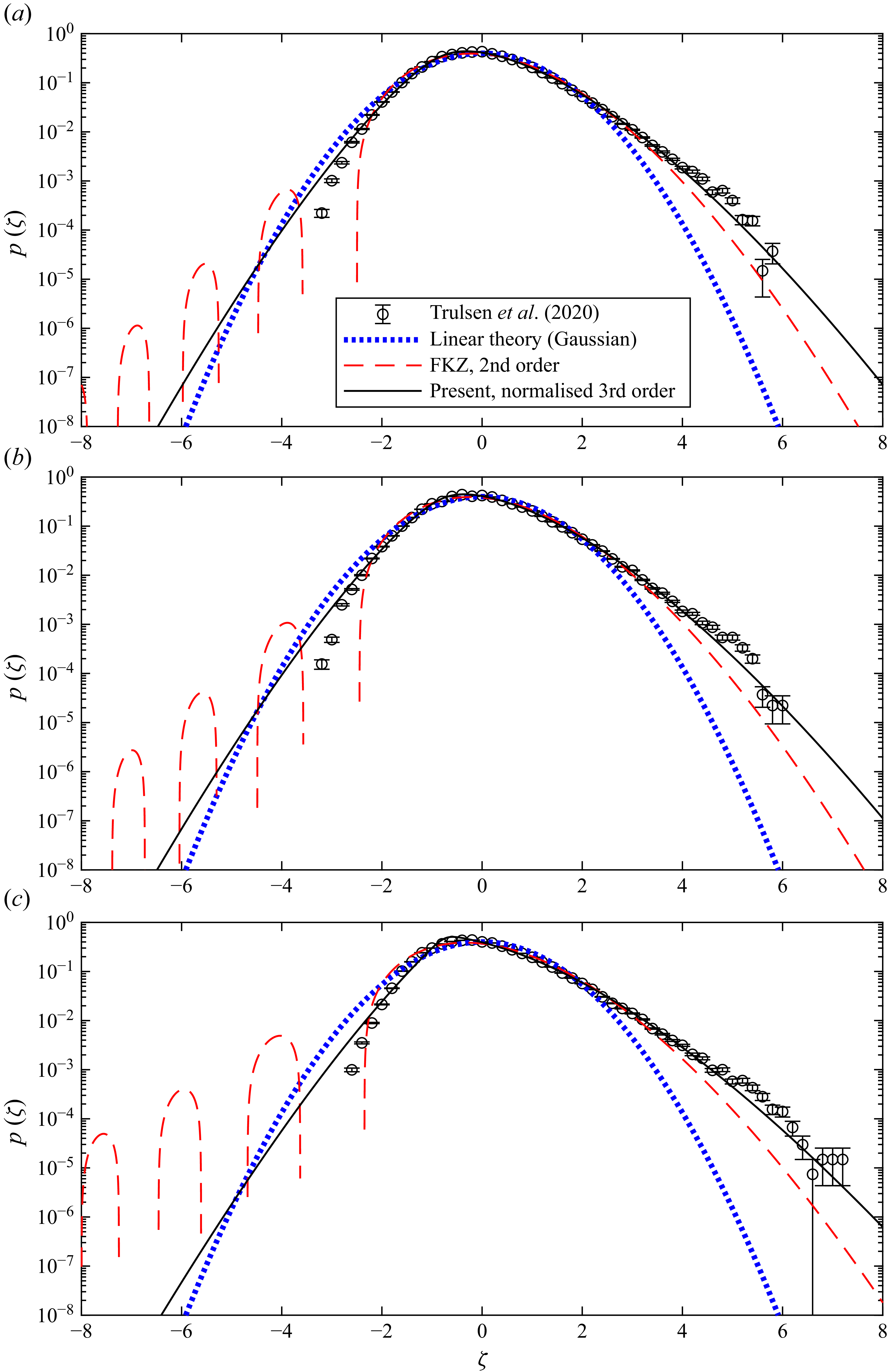
Comparison with selected datasets from run 3 of Trulsen et al. (Reference Trulsen, Raustol, Jorde and Rye2020) at (a) their horizontal position
 $x$
= 1.8 m (
 $\mathcal{S}=0.4778$
,
 $\mathcal{K}=3.6690$
), (b)
 $x$
= 1.85 m (
 $\mathcal{S}=0.5273$
,
 $\mathcal{K}=3.7526$
) and (c)
 $x$
= 2.2 m (
 $\mathcal{S}=0.7888$
,
 $\mathcal{K}=4.194$
).

Three cases having larger skewness from run 3 of Trulsen et al. (Reference Trulsen, Raustol, Jorde and Rye2020) are presented in figure 14. These, respectively, have skewness
 $\mathcal{S}=0.4778$
,
 $0.5273$
and
 $0.7888$
and kurtosis
 $\mathcal{K}=3.6690$
,
 $3.7526$
and
 $4.1940$
. In the first two cases, the positive tail is captured reasonably, if slightly underpredicted, and the negative tail is slightly overpredicted. The final case considered (
 $\mathcal{S}=0.7888$
,
 $\mathcal{K}=4.1940$
) in figure 14(c) corresponds to the most nonlinear point measured by Trulsen et al. (Reference Trulsen, Raustol, Jorde and Rye2020). Even in this very challenging case, the positive tail is still quite reasonably captured (similarly slightly underpredicted) by the new third-order PDF. It is not accurate for negative
 $\zeta$
in this case, however. Overall, the new third-order PDF seemingly represents a substantial improvement over the second-order FKZ distribution (dashed red lines) in all cases considered.
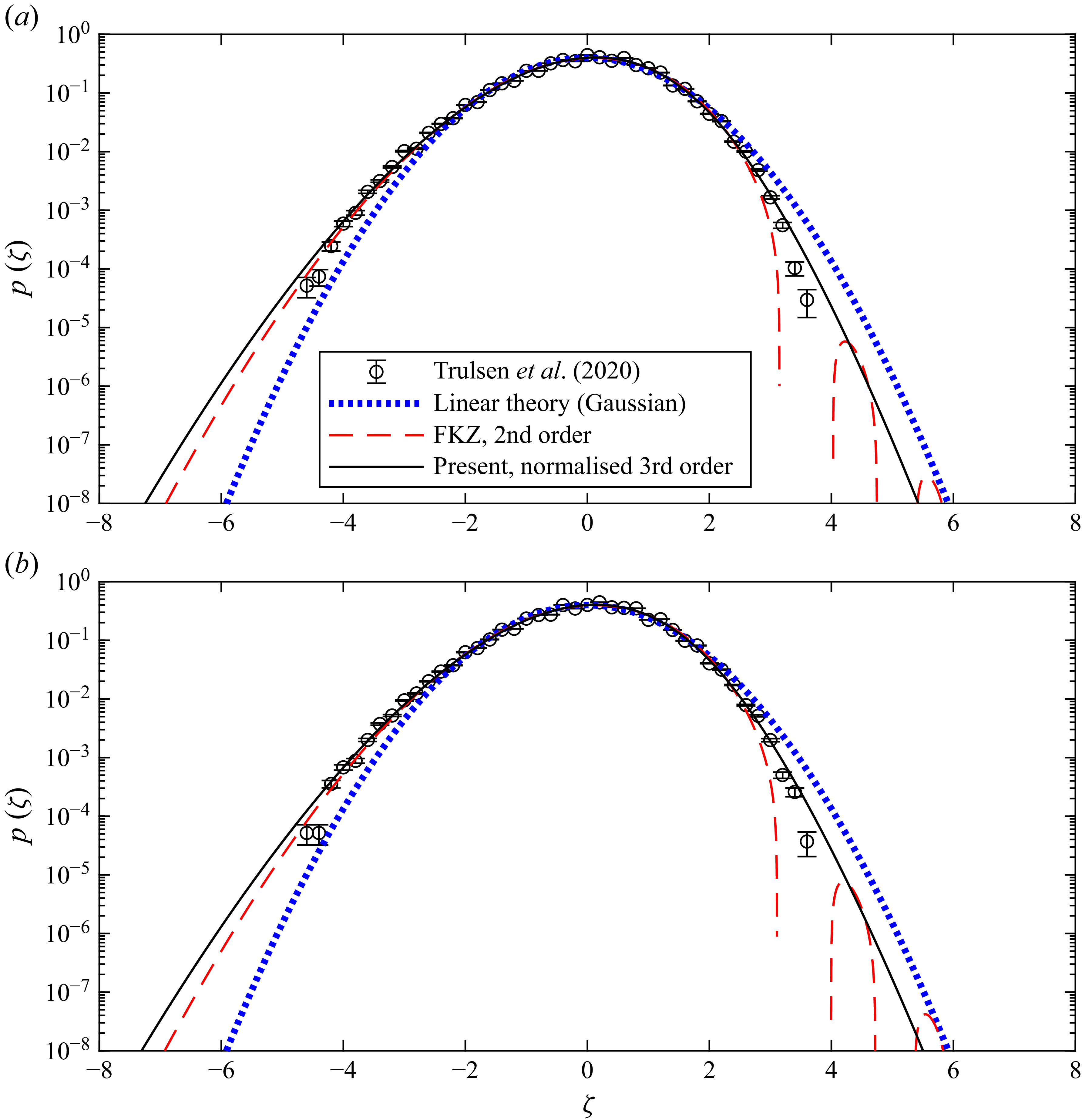
Although somewhat rare in practice, the experiments of Trulsen et al. (Reference Trulsen, Raustol, Jorde and Rye2020) resulted in surface elevations having negative skewness at some positions. It turns out that the present third-order PDF can quite naturally describe such situations. As demonstration of this, we finally make comparison of data from two selected locations from their run 3 where
 $\mathcal{S}\lt 0$
in figure 15. In both cases (respectively having similar skewness
 $\mathcal{S}=-0.2532$
and
 $-0.2599$
, as well as kurtosis
 $\mathcal{K}=3.1277$
and
 $3.1456$
values) results are of similar quality as might be expected from those in figures 13 and 14. Note that for reference comparison with the second-order FKZ distribution in figure 15, we utilise the following generalisation of (3.13):
 \begin{equation} p(\zeta )=\left (\frac {2}{|\kappa _3|}\right )^{1/3} \exp \left (\frac {1}{3\kappa _3^2} + \frac {\zeta }{\kappa _3}\right ) \mbox{Ai}(\chi ), \quad \chi = \left (\frac {2}{|\kappa _3|}\right )^{1/3}\left (\frac {1}{2|\kappa _3|}+\zeta \frac {\kappa _3}{|\kappa _3|}\right ), \end{equation}
which is valid for both positive and negative skewness. This generalisation is credited to Job Dronkers (Mangor & Dronkers Reference Mangor and Dronkers2025). With
 $\mathcal{S}\lt 0$
the unphysical oscillations inherent within the FKZ distribution flip from the negative to the positive tail.
6.4. Assessment of accuracy
From the above, it can be generally surmised that the new third-order PDF presented in the present work maintains accuracy over a range of
 $\zeta$
which becomes more restrictive as the nonlinearity of the wave field is increased. This behaviour is as expected since, as is clear from the asymptotics presented by e.g. Klahn et al. (Reference Klahn, Zhai and Fuhrman2024) (see also Appendix A of the present work), if one goes far enough out in the tails there will always be a point where they becomes dominated by the neglected next cumulant. Based on the comparisons presented above, as well as an additional comparison involving a case with
 $\mathcal{S}\approx 0.2$
(not shown for brevity), the range of
 $\zeta$
where high accuracy is maintained is estimated in table 2. The
 $\zeta$
limits are presented for nonlinear wave fields characterised by round, positive skewness values alone, both for simplicity and since the excess kurtosis tends to scale proportional to
 $\mathcal{S}^2$
. Here the
 $\zeta$
limits have been chosen conservatively, and loosely indicate where deviations from the selected datasets are visually apparent in PDFs presented in the semi-logarithmic fashion utilised throughout the present work. The authors hope that table 2 may be helpful in assessing operational limits of the new theory in practice. It is emphasised that even outside the
 $\zeta$
ranges presented in table 2 the new third-order theory can still be expected to yield significant improvement, for example over the existing second-order theory of FKZ, as is apparent in figures presented throughout the present section.
Summary estimating the range of
 $\zeta$
where the present third-order PDF maintains high accuracy for nonlinear irregular wave fields characterised by selected round skewness
 $\mathcal{S}$
values.

Table 2. Long description
The table has two columns and five rows. The first column is labeled with the variable S and the second column is labeled with the range of the variable zeta. The values in the first column are 0.2, 0.3, 0.4, 0.5, and 0.8. The corresponding values in the second column are -4.5 <= zeta <= 7, -3.5 <= zeta <= 6, -3 <= zeta <= 5, -2.5 <= zeta <= 4, and 0 <= zeta <= 4.
Comparison with selected datasets having negative skewness from run 3 of Trulsen et al. (Reference Trulsen, Raustol, Jorde and Rye2020) at (a)
 $x$
= 3.95 m (
 $\mathcal{S}=-0.2532$
,
 $\mathcal{K}=3.1277$
) and (b)
 $x$
= 3.9 m (
 $\mathcal{S}=-0.2599$
,
 $\mathcal{K}=3.1456$
).

7. Conclusions
This work has developed new saddle-point approximations for the PDF of the surface elevation in nonlinear, irregular seas. These are based on truncated versions of the classical integral formulation of LH63, such that they are free of any assumptions involving uni-directionality of the wave field or narrow-bandedness of the spectrum.
At first (linear) order, it has been shown that the saddle-point approximation results in the Gaussian (normal) distribution, corresponding to the well-known exact solution at this order. Apart from a singularity, at second order the saddle-point approximation has been shown to yield a close match with the exact closed-form theoretical solution of FKZ, based on the Airy function. Asymptotic analysis coincides with the theory in both the positive- and negative-tail limits.
The principal novel results arise at third order, where no exact closed-form solution to the LH63 integral exists. A new closed-form saddle-point approximation of the PDF has been derived, accounting for both skewness and kurtosis. This result is denoted as
 $\tilde {p}(\zeta )$
herein and presented in (3.23). Asymptotic analysis yields the theoretical form of both the positive and negative tails. The positive tail result matches the known form found by Klahn et al. (Reference Klahn, Zhai and Fuhrman2024), while also providing the previously unknown multiplicative prefactor, thus completing the theoretical form of the tails at this order. The positive tail is governed predominantly by kurtosis, and is fundamentally heavier than at second order. Importantly, at third order, the negative tail is free of unphysical oscillations. This resolves a problem plaguing many prior PDFs attempting to statistically describe the surface elevation in nonlinear seas. These include both the second- and third-order Gram–Charlier approximations of LH63, the second-order solution of FKZ as well as the numerically generated results of Klahn et al. (Reference Klahn, Zhai and Fuhrman2024) and Zhai et al. (Reference Zhai, Klahn, Onorato and Fuhrman2025) at third and higher orders.
Being an approximation,
 $\tilde {p}(\zeta )$
does not exactly satisfy the statistical properties of the dimensionless surface elevation
 $\zeta$
(i.e. surface elevation measured about its mean and divided by its standard deviation). Normalisation of
 $\tilde {p}(\zeta )$
yields a proper PDF
 $p(\zeta )$
, having unit integral, zero mean and unit variance. This PDF is presented as (5.6). Moreover, through further (typically minor) modification of the input cumulants
 $\kappa _3$
and
 $\kappa _4$
, PDFs matching exactly the desired skewness
 $\mathcal{S}$
and kurtosis
 $\mathcal{K}$
can be achieved, and the possible combination space has been established. Comparisons against challenging datasets stemming from irregular wave theory, a fully nonlinear wave model as well as laboratory experiments confirm the accuracy of the new third-order PDF. Focus has been on cases involving irregular waves with
 $\mathcal{S}\gt 0.2$
, where it is known that the existing second-order theory (Fuhrman et al. Reference Fuhrman, Klahn and Zhai2023) is insufficient. The comparisons made generally demonstrate that the prediction of the positive tail is more accurate than of the negative tail, for cases with positive skewness. Selected results with negative skewness have also been presented for generality.
A novel perturbation approach, capable of determining asymptotic tail behaviour at any nonlinear order, is finally presented in Appendix A. This method is employed to derive the theoretical positive and negative tails at fourth and fifth orders. These match the forms previously found by Klahn et al. (Reference Klahn, Zhai and Fuhrman2024), while again providing the previously unknown prefactors at these orders. Collectively, the present analysis demonstrates that odd-order truncations to the LH63 integral admit non-oscillatory, decaying negative tails, whereas even-order truncations do not.
Acknowledgements
This research has been financially supported by the Independent Research Fund Denmark project STORM: STatistics and fOrces on stRuctures from extreMe water waves in finite depth (grant ID: 10.46540/2035-00064B). This support is greatly appreciated.
Declaration of interests
The authors report no conflict of interest.
Appendix A. Asymptotic tail solutions at fourth and fifth order
In this appendix we present a novel perturbation solution, which enables determination of the asymptotic positive and negative tails at any desired order. We have specifically confirmed that the methodology presented below leads to the same second- and third-order tails as presented, respectively, in §§ 3.2 and 3.3. As these were already determined directly from asymptotic analysis in the main text, we therefore focus on determining the fourth- and fifth-order tails in this appendix. The results extend those of Klahn et al. (Reference Klahn, Zhai and Fuhrman2024), who found the form of the positive tails at third and higher orders using the method of dominant balance, but with the multiplicative prefactors left unknown.
A.1. Fourth order
Truncated at fourth order, (3.2) corresponds to
 \begin{equation} \phi (s)=\mbox{i}\zeta s -\epsilon ^3\frac {s^2}{2} + \epsilon ^2\frac {\mbox{i}\kappa _3}{6} s^3 + \epsilon \frac {\kappa _4}{24}s^4 - \frac {\mbox{i}\kappa _5}{120}s^5, \end{equation}
where
 $\kappa _5$
is the fifth cumulant, which is as indicated in table 2 of Klahn et al. (Reference Klahn, Zhai and Fuhrman2024). Here
 $\epsilon$
markers have been introduced to keep track of the relative importance of terms at the tail limits. Those introduced just above ensure, for example, that extreme tails will be governed by a balance between the
 $\kappa _5$
term and the first term of the right-hand side, with the excess kurtosis
 $\kappa _4$
term coming into play at the next order, and so on. The saddle points now correspond to those where
 \begin{equation} \phi ^\prime (\tilde {s}) = \mbox{i}\zeta -\epsilon ^3\tilde {s} + \epsilon ^2\frac {\mbox{i}\kappa _3}{2}\tilde {s}^2 + \epsilon \frac {\kappa _4}{6}\tilde {s}^3 - \frac {\mbox{i}\kappa _5}{24}\tilde {s}^4=0. \end{equation}
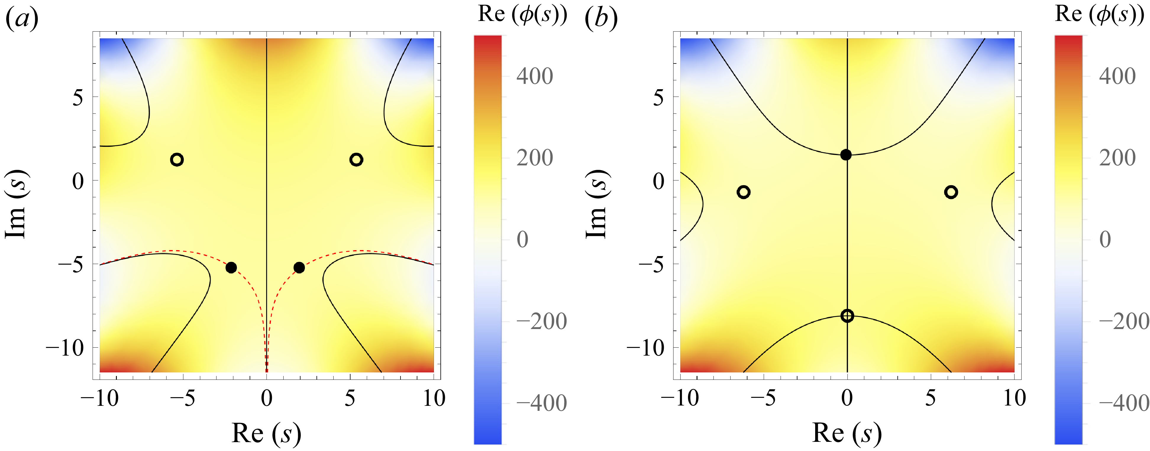
Their exact values are lengthy, and are not presented here. Their numerically evaluated positions in the complex plane are exemplified in figure 16 (parameters indicated in the caption) in a similar fashion to figures 1 and 3.
Plots showing the fourth-order saddle-point positions (black circles) in the complex plane, contours where
 ${\rm Im} (\phi (s))=0$
(full black lines) as well as
 ${\rm Re} (\phi (s))$
(colours). Results use fixed
 $\kappa _3=0.3$
,
 $\kappa _4=0.2$
and
 $\kappa _5=0.1$
with (
 $a$
)
 $\zeta =-4$
and (
 $b$
)
 $\zeta =2$
. The dashed red lines in (
 $a$
) depict additional contours where
 ${\rm Im} (\phi (s))={\rm Im} (\phi (\tilde {s}))\neq 0$
for the two contributing saddle points (filled circles).

With the underlying goal of determining the form of the asymptotic tails, we expand the saddle points as a perturbation series:
 \begin{equation} \tilde {s} = \tilde {s}_0 + \epsilon \tilde {s}_1 + \epsilon ^2\tilde {s}_2 + \epsilon ^3\tilde {s}_3 + \epsilon ^4\tilde {s}_4 + \cdots .\end{equation}
We now insert (A3) into (A2) and collect terms having various powers of
 $\epsilon$
. Eliminating
 $O(1)$
terms requires that
 \begin{equation} \mbox{i}\zeta - \frac {\mbox{i}\tilde {s}_0^4\kappa _5}{24} = 0. \end{equation}
This has four potential solutions. From inspection of figure 16(b) it is evident that only one (i.e. the largest purely imaginary one) will contribute to the positive tail, with leading-order component
 \begin{equation} \tilde {s}_0 = \frac {\mbox{i}2^{3/4}\boldsymbol{\cdot }3^{1/4}\zeta ^{1/4}}{\kappa _5^{1/4}}. \end{equation}
Eliminating the next several powers of
 $\epsilon$
similarly requires that
 \begin{align} \tilde {s}_1 = -\frac {\mbox{i}\kappa _4}{\kappa _5}, \\[-28pt] \nonumber \end{align}
 \begin{align} \tilde {s}_2 = -\mbox{i}\frac {(3/2)^{3/4}(2\kappa _3\kappa _5 - \kappa _4^2)}{2\zeta ^{1/4}\kappa _5^{7/4}}, \\[-28pt] \nonumber \end{align}
 \begin{align} \tilde {s}_3 = -\mbox{i}\frac {\kappa _4^3 - 3\kappa _3\kappa _4\kappa _5 + 3\kappa _5^2}{\sqrt {6\zeta }\kappa _5^{5/2}}, \\[-28pt] \nonumber \end{align}
 \begin{align} \tilde {s}_4 = \mbox{i}\frac {(3/2)^{1/4}(5\kappa _4^4 - 20\kappa _3\kappa _4^2\kappa _5 + 12\kappa _3^2\kappa _5^2 + 16\kappa _4\kappa _5^2)}{32\zeta ^{3/4}\kappa _5^{13/4}} \\[0pt] \nonumber \end{align}
and
 $\tilde {s}_5=0$
. Inserting all of the above into (2.6), utilising that
 \begin{equation} \phi ^{\prime \prime }(\tilde {s})|_{\epsilon =0}=-\frac {\mbox{i}\kappa _5\tilde {s}_0^3}{6}, \end{equation}
and discarding the
 $\epsilon$
markers, leads to the final result:
 \begin{equation} p(\zeta )\sim \frac {C}{\zeta ^{3/8}}\exp \left (a_1\zeta ^{5/4} + a_2\zeta + a_3\zeta ^{3/4} + a_4\zeta ^{1/2} + a_5\zeta ^{1/4} + a_6 + \cdots \right ), \end{equation}
where the prefactor is
 \begin{equation} C = \left (\frac {3}{2}\right )^{1/8} \frac {1}{2\sqrt {\pi }\kappa _5^{1/8}}. \end{equation}
The first five
 $a_i$
coefficients are as given in table 1 of Klahn et al. (Reference Klahn, Zhai and Fuhrman2024), with
 \begin{equation} a_6=\frac {8\kappa _4^5-40\kappa _3\kappa _4^3\kappa _5 + 45\kappa _3^2\kappa _4\kappa _5^2 + 30\kappa _4^2\kappa _5^2-45\kappa _3\kappa _5^3}{15\kappa _5^4}. \end{equation}
It was not possible to determine the prefactor
 $C$
and coefficient
 $a_6$
using the method of dominant balance employed by Klahn et al. (Reference Klahn, Zhai and Fuhrman2024); thus these are new, and complete the asymptotic result for the positive tail at fourth order. With dominant term proportional to
 $\zeta ^{5/4}$
in the exponential, this tail is fundamentally even heavier than at third order, as emphasised by Klahn et al. (Reference Klahn, Zhai and Fuhrman2024). Even more terms than those indicated above can be found by continuing this procedure to eliminate even higher powers of
 $\epsilon$
, should these be desired.
To find the negative tail behaviour in the limit
 $\zeta \rightarrow -\infty$
we repeat the analysis above, but with
 $\zeta =-|\zeta |$
inserted into
 $\phi (s)$
. Similar to before, this leads to four possible leading-order saddle points. From inspection of figure 16(a), similar to second order, it is evident that the lower two (in the complex plane) will contribute to the negative tail. To begin we first choose the one corresponding to
 \begin{equation} \tilde {s}_{0,1} = -\frac {2^{3/4} (-3)^{1/4}|\zeta |^{1/4}}{\kappa _5^{1/4}}. \end{equation}
Successively eliminating higher powers of
 $\epsilon$
and inserting all results into (2.6) leads to
 \begin{align} p_1(\zeta )\sim \frac {2^{1/4}}{\sqrt {1+\mbox{i}}}\frac {C}{|\zeta |^{3/8}} \exp \left ( \frac {1-\mbox{i}}{\sqrt {2}}a_1|\zeta |^{5/4} - a_2|\zeta | + \frac {1+\mbox{i}}{\sqrt {2}}a_3|\zeta |^{3/4} \right . \nonumber \\ \left . - \mathrm{i}a_4|\zeta |^{1/2} - \frac {1-\mbox{i}}{\sqrt {2}}a_5|\zeta |^{1/4} + a_6 + \cdots \right ), \end{align}
which gives complex results. Alternatively, using the other contributing leading-order saddle point
 \begin{equation} \tilde {s}_{0,2} = -\mbox{i}\frac {2^{3/4} (-3)^{1/4}|\zeta |^{1/4}}{\kappa _5^{1/4}}, \end{equation}
after following the same procedure as outlined above, leads to
 $p_2(\zeta )=p_1(\zeta )^*$
, where the asterisk indicates complex conjugation. Adding these together, as in (2.7), leads to the fourth-order asymptotic negative-tail solution:
 \begin{equation} p(\zeta )\sim p_1(\zeta ) + \text{c.c.} = 2{\rm Re} ({p_1(\zeta )}). \end{equation}
This result is new. Note that the imaginary part of the complex factor, e.g. in front of
 $a_1$
(among other terms), will result in unphysical oscillatory behaviour in the negative tail at this order. This behaviour is consistent with expectations from figure 16(a), since both contributing saddle points lie off a
 ${\rm Im} (\phi (s))=0$
contour. Similar to second order, there are no physical (non-oscillatory, decaying with
 $|\zeta |$
) solutions to the LH63 integral for the negative tail at fourth order. From this it is clear that the saddle point chosen for the positive-tail asymptotics lies on the
 ${\rm Im} (\phi (s))=0$
contour (figure 16
b), whereas none do in the negative tail (figure 16
a), making oscillations in the negative tail structurally inevitable. We conjecture that this conclusion pertains to all even-order truncations of the LH63 integral, though we do not consider those beyond fourth in the present work.
A.2. Fifth order
At arbitrary order
 $N$
the integral form of the PDF may be written with the argument in the exponential function corresponding to the summation
 \begin{equation} \phi (s) = \mbox{i}\zeta s-\epsilon ^{(N-1)}\frac {s^2}{2} + \sum _{n=3}^{N+1}\epsilon ^{(N-n+1)}\frac {(-\mbox{i}s)^n}{n!}\kappa _n. \end{equation}
As shown by Klahn et al. (Reference Klahn, Zhai and Fuhrman2024), there using the method of dominant balance, the solution for the positive tails corresponds generally to
 \begin{equation} p(\zeta )\sim \frac {C}{\zeta ^{a_0}}\exp \left (a_1\zeta ^{(N+1)/N} + a_2\zeta ^{N/N} + a_3\zeta ^{(N-1)/N} + \cdots \right ). \end{equation}
At fifth order
 $(N=5)$
, (A18) leads to
 \begin{equation} \phi (s)=\mbox{i}\zeta s-\epsilon ^4\frac {s^2}{2} + \epsilon ^3\frac {\mbox{i}\kappa _3}{6} s^3 + \epsilon ^2\frac {\kappa _4}{24}s^4 - \epsilon \frac {\mbox{i}\kappa _5}{120}s^5 - \frac {\kappa _6}{720}s^6, \end{equation}
where the sixth cumulant
 $\kappa _6$
is as indicated in table 2 of Klahn et al. (Reference Klahn, Zhai and Fuhrman2024). The saddle points correspond to those where
 \begin{equation} \phi ^\prime (\tilde {s})=\mbox{i}\zeta -\epsilon ^4\tilde {s} + \epsilon ^3\frac {\mbox{i}\tilde {s}^2\kappa _3}{2} + \epsilon ^2\frac {\kappa _4\tilde {s}^3}{6} - \epsilon \frac {\mbox{i}\kappa _5\tilde {s}^4}{24} - \frac {\tilde {s}^5\kappa _6}{120}=0, \end{equation}
Plots showing the fifth-order saddle-point positions (black circles) in the complex plane, contours where
 ${\rm Im} (\phi (s))=0$
(full black lines) as well as
 ${\rm Re} (\phi (s))$
(colours). Results use fixed
 $\kappa _3=0.3$
,
 $\kappa _4=0.2$
,
 $\kappa _5=0.1$
and
 $\kappa _6=0.05$
with (
 $a$
)
 $\zeta =-4$
and (
 $b$
)
 $\zeta =2$
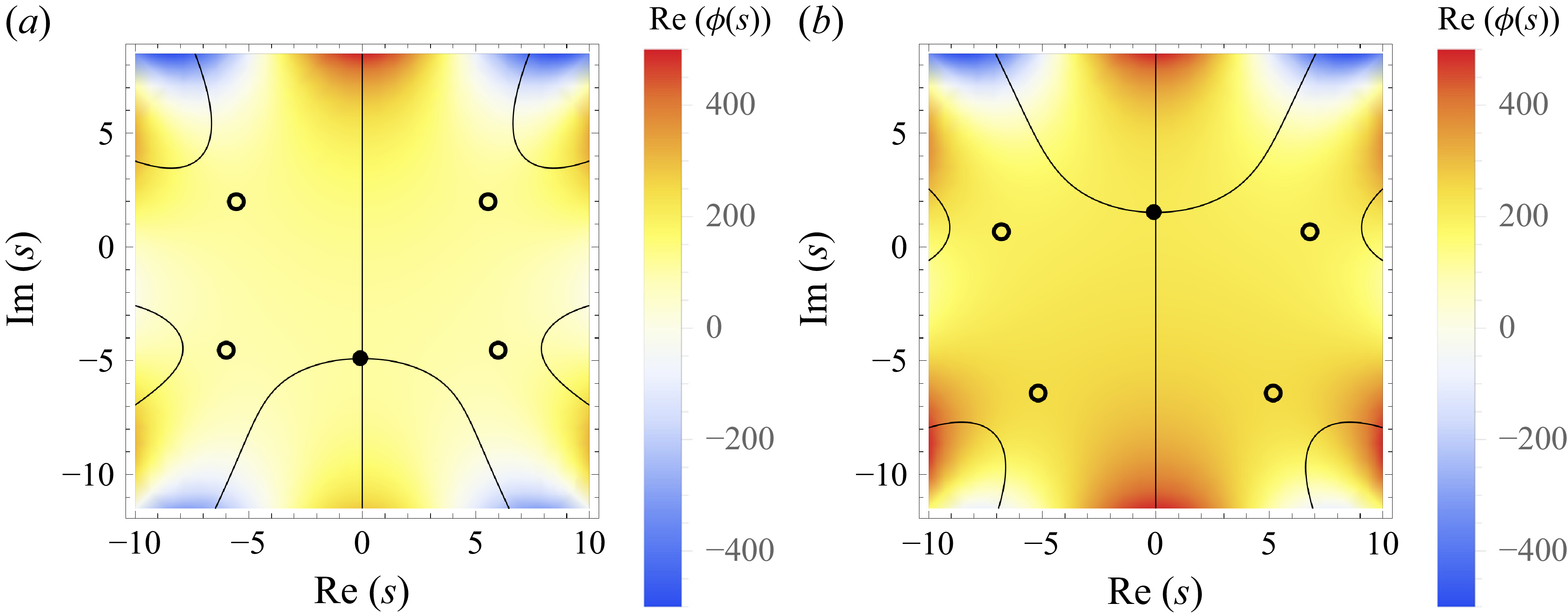
.

with five potential solutions. Exact solutions (determined numerically) are exemplified in the complex plane in figure 17 (parameters as indicated in the caption), in a fashion similar to that previously presented in figures 1, 3 and 16. From inspection of figure 17 it is evident that there will be a single (purely imaginary) saddle point contributing to both the positive- and negative-tail solutions. Similar to third order (figure 3), as this saddle point lies directly on a
 ${\rm Im} (\phi (s))=0$
contour (black lines), which clearly represents a path of steepest descent, both positive- and negative-tail solutions are expected to be well behaved at fifth order.
To obtain analytical tail solutions, we follow the same procedure as at fourth order. Expanding the the saddle point as in (A3), inserting this into (A21) and collecting
 $O(1)$
terms now leads to five options for the leading-order saddle point. To find the positive tail we choose the contributing (purely imaginary) one, corresponding to
 \begin{equation} \tilde {s}_0 = \mbox{i}\frac {2^{3/5}\boldsymbol{\cdot }15^{1/5}\zeta ^{1/5}}{\kappa _6^{1/5}}. \end{equation}
Successively eliminating powers of
 $\epsilon$
, inserting all results into (2.6), utilising that
 \begin{equation} \phi ^{\prime \prime }(\tilde {s})|_{\epsilon =0}= -\frac {\kappa _6\tilde {s}_0^4}{24}, \end{equation}
and finally discarding the
 $\epsilon$
markers, leads to the following result for the positive tail:
 \begin{equation} p(\zeta )\sim \frac {C}{\zeta ^{2/5}}\exp \left (a_1\zeta ^{6/5} + a_2\zeta + a_3\zeta ^{4/5} + a_4\zeta ^{3/5} + a_5\zeta ^{2/5} + a_6\zeta ^{1/5} + a_7 + \cdots \right ). \end{equation}
This result is fully consistent with that found previously by Klahn et al. (Reference Klahn, Zhai and Fuhrman2024). With dominant term proportional to
 $\zeta ^{6/5}$
in the exponential function, the fifth-order tail is fundamentally even heavier than at fourth order, as previously emphasised by Klahn et al. (Reference Klahn, Zhai and Fuhrman2024). The first six
 $a_i$
coefficients are as presented in their table 1, and
 \begin{equation} a_7=-\frac {\varLambda } {144\kappa _6^5} \end{equation}
with
 \begin{align} \varLambda =& 125\kappa _5^6 - 750\kappa _4\kappa _5^4\kappa _6 + 600\kappa _3\kappa _5^3\kappa _6^2 + 120\kappa _5^2(10\kappa _4^2-3\kappa _6)\kappa _6^2 \nonumber \\ & -1440\kappa _3\kappa _4\kappa _5\kappa _6^3(-20\kappa _4^3+27\kappa _3^2\kappa _6+36\kappa _4\kappa _6). \end{align}
The (previously unknown) prefactor corresponds to
 \begin{equation} C = \frac {3^{1/10}}{2^{1/5} 5^{2/5}\sqrt {\pi }\kappa _6^{1/10}}. \end{equation}
This result thus completes the determination of the theoretical fifth-order positive tail. As before, even higher-order
 $a_i$
coefficients can be determined by eliminating larger powers of
 $\epsilon$
, should these be desired.
To find the negative tail in the limit
 $\zeta \rightarrow -\infty$
we insert
 $\zeta =-|\zeta |$
into
 $\phi (s)$
, as before. There are again five possible leading-order saddle points. We consider the contributing one corresponding to
 \begin{equation} \tilde {s}_0 = -\mbox{i}\frac {2^{3/5}\boldsymbol{\cdot }15^{1/5}|\zeta |^{1/5}}{\kappa _6^{1/5}}. \end{equation}
Following the procedure outlined above ultimately leads to the negative tail:
 \begin{equation} p(\zeta )\sim \frac {C}{|\zeta |^{2/5}}\exp \left (a_1|\zeta |^{6/5} - a_2|\zeta | + a_3|\zeta |^{4/5} - a_4|\zeta |^{3/5} + a_5|\zeta |^{2/5} - a_6|\zeta |^{1/5} + a_7 - \cdots \right ). \end{equation}
This result is new. Similar to third order, we find a physical (non-oscillatory, decaying with
 $|\zeta |$
) solution for the negative tail at fifth order. It is again formally just as heavy as the positive tail, though the sign reversal on the even
 $a_i$
terms will cause it to decay more rapidly with
 $|\zeta |$
in practice. More terms than shown within the exponential function can again easily be found by eliminating higher powers of
 $\epsilon$
, if desired. This may be necessary to obtain tail convergence, depending on the case.
Collectively, it now seems clear that truncating
 $\phi (s)$
at even orders inevitably leads to oscillatory solutions in the negative tail. These can be remedied by truncating
 $\phi (s)$
at the next odd order, which requires knowledge of the next cumulant. This has been shown up to fifth order in the present work, though we conjecture that this trend will continue at even higher orders.
 Im(ϕ(s))=0
 Re(ϕ(s))
 κ3=0.3
 a
 ζ=−2
 b
 ζ=ζcrit=−1.6¯
 c
 ζ=0
 d
 ζ=2
 a
 Im(ϕ(s))=Im(ϕ(s~))≠0
 κ3=0.3
 ζ=ζcrit=−1/(2κ3)=−1.6¯
 Im(ϕ(s))=0
 Re(ϕ(s))
 κ3=0.3
 κ4=0.2
 a
 ζ=−2
 b
 ζ=ζcrit=−1.275
 c
 ζ=0
 d
 ζ=2
 p~
 κ3=0.3
 κ4=0.2
 κ3=0.3
 p~(ζ)
 κ3=0.3
 κ4=0.2
 a
 I~
 b
 μ~
 c
 σ~2
 d
 S~
 e
 K~−3
 κ3
 κ4
 p~(ζ)
 κ4=κ32/2
 p~(ζ)
 a
 S
 b
 K−3
 κ3
 κ4
 p(ζ)
 κ4=κ32/2
 a
 κ3
 b
 κ4
 S
 K−3
 p(ζ)
 K−3=S2/2
 p(ζ)
 |S|
 K−3
 p~(ζ)
 κ3
 κ4
 κ3
 κ4
 p(ζ)
 S
 K−3
 I=1
 μ=0
 σ2=1
 ND
 ND=∞
 S=0.3355
 K=3.1902
 S=0.2306
 K=3.0601
 S=0.3974
 K=3.2120
 x
 S=0.3021
 K=3.3234
 x
 S=0.3585
 K=3.2818
 x
 S=0.4778
 K=3.6690
 x
 S=0.5273
 K=3.7526
 x
 S=0.7888
 K=4.194

 ζ
 S
 x
 S=−0.2532
 K=3.1277
 x
 S=−0.2599
 K=3.1456
 Im(ϕ(s))=0
 Re(ϕ(s))
 κ3=0.3
 κ4=0.2
 κ5=0.1
 a
 ζ=−4
 b
 ζ=2
 a
 Im(ϕ(s))=Im(ϕ(s~))≠0
 Im(ϕ(s))=0
 Re(ϕ(s))
 κ3=0.3
 κ4=0.2
 κ5=0.1
 κ6=0.05
 a
 ζ=−4
 b
 ζ=2


