1. Introduction
The cable-driven continuum robot (CDCR) with multi-degree-of-freedom is a flexible manipulator inspired by biological structures, such as elephant trunks and octopus tentacles [Reference Tian, Gao and Gong1–Reference Qin, Wang, Li, Ji, Wu, Yang and Wen3]. CDCRs can be adjusted by changing the length of driving cables, making it particularly suitable for complex tasks. Recently, with the rapid development of robotic technology, CDCRs have been increasingly utilized in various fields such as laparoscopic surgery [Reference Mao, Yang, Tian, Shen, Wang, Zhang and Xie4], space station maintenance [Reference Zou and Fan5], and rehabilitation [Reference Polygerinos, Wang, Galloway, Wood and Walsh6]. However, the application of CDCRs in these complex environments requires high trajectory planning and tracking capabilities to ensure safety and accuracy.
Trajectory planning is crucial for achieving safe and stable obstacle avoidance [Reference Wang, Yang, Han, Li, He, Zhao and Wu7]. It is necessary to achieve real-time recognition and avoidance of obstacles in complex 3D environments and reach designated locations [Reference Wang, Zhang, Cao, Hu, Wang, Deng and Tang8]. Trajectory planning algorithms mainly include the following types: the Dijkstra algorithm, A* algorithm, probabilistic roadmaps (PRMs) [Reference Huang, Wang, Han and Xu9], artificial potential field (APF) [Reference Zhu, Zhang, Zong and Li10, Reference Duhé, Victor and Melchior11], and rapidly-exploring random trees (RRTs) [Reference Shang, Liu, Qin, Guo and Li12, Reference Yang and Lin13], as well as numerical optimization methods such as model predictive control (MPC) [Reference Köhler, Kötting, Soloperto, Allgöwer and Müller14, Reference Meng, Zhang and Li15]. In the past few years, MPC has emerged as an efficient method for addressing multi-constraint issues, rendering it well-suited for trajectory planning [Reference Zhang, Yao and Tian16, Reference Zhang and Shi17]. The trajectory planning algorithm based on MPC is extensively employed in various applications. The APF algorithm, which generates repulsive forces around obstacles to prevent collisions and attractive forces toward target points, is widely used in trajectory planning. Therefore, the combination of APF and MPC can ensure the generation of reliable and safe obstacle avoidance trajectories.
Numerous scholars have proposed diverse algorithms based on MPC for trajectory planning with obstacle avoidance. Lee et al. [Reference Lee, Chung, Kim and Kim18] proposed a nonlinear MPC (NMPC) algorithm that considers obstacles as a combination of multi-line segments and incorporates these segments as obstacle avoidance constraints for NMPC, thereby significantly reducing computational burden. However, it should be noted that this algorithm relies solely on hard constraints, which may result in infeasible solutions and cause collisions with obstacles. Li et al. [Reference Li, Wang, Yang and Zhao19] designed an event-triggered MPC (EMPC) to reduce the computational burden associated with the optimization process. However, similar to [Reference Lee, Chung, Kim and Kim18], the utilization of hard constraints to avoid obstacles poses a risk of collision. Since hard constraints must be strictly observed, once these constraints are violated, it will lead to infeasible solutions. Therefore, Zhu et al. [Reference Zhu, Mao, Han, Zhang and Yang20] proposed the APF-MPC algorithm, which adopts APF as the penalty term of the objective function to avoid infeasible solutions. When the soft constraint is violated, APF will punish the unexpected behavior. However, trajectory planning controllers based on APF-MPC may encounter local optima in multi-obstacle environments. APF-MPC-based trajectory planning controllers often encounter the issue of local optima in multi-obstacle environments. This is because MPC is operated within a limited range of predictions and cannot obtain a global optimal solution. The whale optimization algorithm (WOA) is an optimization technique that draws inspiration from the hunting pattern exhibited by natural pods of whales [Reference Dai, Yu, Zhang, Zhan and Zheng21]. WOA can be introduced into MPC to alleviate the problem of local optima, but it is inefficient in obtaining the global optimal solution. To improve the convergence speed and global search capability of WOA, this paper designs an improved whale optimization algorithm (IWOA) by enhancing the search mechanism and parameter adjustment of the WOA. The combination of IWOA and APF-MPC (APF-IMPC) can generate safe and feasible trajectories as well as achieve high-precision trajectory tracking control of CDCRs in multi-obstacle environments.
Another issue is that most existing trajectory planning methods often ignore trajectory smoothness, resulting in low tracking efficiency and high collision risk with obstacles [Reference Wan, Xu and Ye22]. To address the issue of non-smooth trajectories, various algorithms have been employed to optimize trajectory smoothness, including Bézier curves [Reference Tring, Moosavi, Dipoppa and Ringach23], B-spline curves [Reference Wang, Tang and Deng24, Reference Wang and Guo25], and cubic polynomials [Reference Dinçer and Çevik26]. B-spline curves can be accurately depicted by formulas, making it easy to be modified by control points. The local modification characteristic of B-splines has garnered the favor of numerous researchers for its adaptability. However, the convex hull property of B-spline curves makes it confined within the convex hull of the control polyline, which may result in potential collisions with obstacles during multi-line trajectory optimization. To address the problem of collision with obstacles after B-spline optimization, we propose a two-layer B-spline optimization framework. The first layer adopts B-spline to elevate the smoothness of the collision-free trajectory generated by APF-IMPC. If the trajectory still has a risk of collision with obstacles, the second-level adjustment framework will be activated.
The main achievements of this paper can be summarized as follows:
-
1) This paper presents a comprehensive framework that integrates an APF-based IMPC with a two-layer B-spline optimization strategy. This innovative framework enhances trajectory planning and tracking performance of CDCRs in multi-obstacle environments.
-
2) APF is used as the penalty term of the objective function to ensure the generation of a safe and feasible trajectory. Moreover, IWOA is introduced to overcome the local optima of traditional MPC. By incorporating IWOA, APF-IMPC guarantees the generation of global optimal solutions in the trajectory planning process.
-
3) To improve trajectory smoothness, a novel two-layer B-spline optimization framework is introduced. The first layer can make the trajectory smoother in a relatively simple environment. The second layer will adjust the control points to address any remaining collision issues, ensuring that safe and smooth trajectories are generated in environments with multi-obstacle and narrow passages.
The remaining sections of this article are structured as follows: the kinematic model of the CDCR is discussed in Section 2. Trajectory planning is presented in Section 3. Trajectory tracking is covered in Section 4. The validation of the proposed algorithm and the experimental results are detailed in Sections 5 and 6, respectively. In Section 7, the conclusive statement is ultimately presented.
2. Kinematic modeling
The CDCR consists of a series of flexible joints and four cables that run through each disk. The pose of the CDCR is controlled by pulling these cables, as shown in Figure 1.
Structure of the CDCR.

Figure 1. Long description
A diagram of a cable-driven continuum robot. The diagram illustrates the structure of the robot, highlighting its flexible backbone, joint disks, stainless steel springs, and cables. The flexible backbone runs through the center of the robot, with joint disks and stainless steel springs arranged along its length. Cables are threaded through the springs and disks, allowing for the adjustment of the robot’s shape. The diagram includes coordinate systems at different points along the robot, labeled as O, O0, and O1, with corresponding axes x0, y0, z0, x1, y1, and z1. Angles alpha and beta are indicated, showing the possible range of motion and flexibility of the robot.
The CDCR is depicted in Figure 1. Where α is the bending angle and β is the rotation angle. The robot is composed of a joint disk and a flexible backbone made of silicone rubber. Four high-strength polyethylene fiber cables are evenly distributed at an interval of 90° along the length of the backbone.
It should be noted that the CDCR is nonlinear. Assuming a consistent curvature–a widely adopted and validated approximation for continuum robots operating under no-load or light-payload conditions [Reference Webster and Jones27]–the radius of curvature for the four driving ropes can be represented as:
 \begin{equation} \zeta _{i}=\zeta -r\cdot \cos \beta _{i} \end{equation}
where ζ and ζi (i = 1, 2…4) are the bending curvature radius of the flexible support and the ith cable, respectively. r is the radius of the indexing circle where the cable hole of the joint disk is located.
 $\beta _{i}$
is the rotational angle of the ith cable generated by the driving cable.
 $\beta=\beta _{i} + (i-1)$
π/2. According to the parallel characteristics of the driving cable, the length variation
 $\Delta L_{i}$
of the four driving cables can be deduced as follows:
 \begin{equation} \Delta L_{i}=L-L_{i}=(\zeta -\zeta _{i})\alpha =r\alpha \cdot \cos \beta _{i} \end{equation}
where L and
 $\mathit{L}_{\mathit{i}}$
are the single joint length of the robot and the cable length of the ith driving cable, respectively.
According to (2), we can get
 \begin{align} \beta =\arctan ({\unicode[Arial]{x0394}} L_{i+1}/{\unicode[Arial]{x0394}} L_{i}) \\[-8pt] \nonumber \end{align}
 \begin{align} \alpha ={\unicode[Arial]{x0394}} L_{i}/(r\cdot \cos \beta ) \\[10pt] \nonumber \end{align}
C t = [x, y, z]T is the position vector of the end effector. The kinematic model of the CDCR is denoted by:
 \begin{equation} \mathbf{C}_{\mathrm{t}}=\left[\left(\frac{L}{\alpha }\right)\cos \beta \left(1-\cos \alpha \right)\left(\frac{L}{\alpha }\right)\sin \beta \left(1-\cos \alpha \right)\left(\frac{L}{\alpha }\right)\sin \alpha \right]^{\mathrm{T}} \end{equation}
3. Trajectory planning with obstacle avoidance
This section presents an innovative nonlinear APF-IMPC controller to generate obstacle avoidance trajectories in multi-obstacle environments. APF is adopted as the penalty term of the objective function to avoid infeasible solutions caused by only using hard constraints. The utilization of IWOA as the optimization process of MPC solves the problem of local optima. The combination of APF and IMPC ensures the generation of collision-free trajectories for the CDCR. Furthermore, the designed two-layer B-spline optimization framework improves trajectory smoothness and safety. This significantly enhances tracking performance. Figure 2 illustrates the flow chart of the collision-free trajectory planning strategy.
Diagram of the obstacle avoidance strategy.

3.1. APF formation
To create an APF potential field, the penalty cost is defined as the repulsive force between the CDCR and obstacles to ensure that the planned trajectory closely follows the desired trajectory while maintaining a safe distance from obstacles.
Let
 $l(\mathbf{s},\mathbf{s}_{\text{goal}})$
represents the Euclidean distance between the CDCR and the desired position. The current position is denoted as
 $\mathbf{s}$
and the goal position is denoted as
 $\mathbf{s}_{\text{goal}}$
. The attractive field
 $U_{\mathrm{at}}$
is as follows:
 \begin{align} U_{\mathrm{at}}=\begin{cases} \dfrac{1}{2}M_{\mathrm{at}}l^{2}\left(\mathbf{s},\mathbf{s}_{\text{goal}}\right) & ,l\left(\mathbf{s},\mathbf{s}_{\text{goal}}\right)\lt l_{\mathrm{g}}\\[5pt] {\varepsilon} _{\mathrm{apf}}M_{\mathrm{at}}l(\mathbf{s},\mathbf{s}_{\text{goal}}) & ,l(\mathbf{s},\mathbf{s}_{\text{goal}})\geq l_{\mathrm{g}} \end{cases} \frac{-b\pm \sqrt{b^{2}-4ac}}{2a} \end{align}
where
 $M_{\mathrm{at}}$
is the attractive coefficient, and
 $l_{\mathrm{g}}$
represents the maximum value of the attract force range.
 ${\varepsilon} _{\mathrm{apf}}$
is a constant coefficient. The gravitational force
 $F_{\mathrm{at}}$
generated by the attractive field
 $U_{\mathrm{at}}$
can be calculated by the following:
 \begin{align} F_{\mathrm{at}}=-\nabla U_{\mathrm{at}}=\begin{cases} -M_{\mathrm{at}}l(\mathbf{s},\mathbf{s}_{\text{goal}}), & l(\mathbf{s},\mathbf{s}_{\text{goal}})\lt l_{\mathrm{g}}\\[4pt] -{\varepsilon} _{\mathrm{apf}}M_{\mathrm{at}}l(\mathbf{s},\mathbf{s}_{\text{goal}}), & l(\mathbf{s},\mathbf{s}_{\text{goal}})\geq l_{\mathrm{g}} \end{cases} \end{align}
The repulsive potential field is generated near the obstacle. The diagram of the repulsive potential field is shown in Figure 3. As the CDCR gradually approaches the obstacle, it will enter the repulsive field, which subsequently exerts a force that pushes the CDCR away from the obstacle. This process facilitates stable navigation around obstacles by mitigating negative impacts caused by inertia. The repulsive potential field
 $U_{j,\mathrm{ru}}$
of the obstacle is expressed as:
Schematic diagram of APF repulsive potential field (the obstacle is located at a lateral distance of 6 cm).

 \begin{align} U_{j,\mathrm{ru}}=\left\{\begin{array}{cc} \dfrac{1}{2}M_{\mathrm{ru}}\left(\dfrac{1}{l(\mathbf{s},\mathbf{s}_{j,\mathrm{obs}})}-\dfrac{1}{l_{\min }}\right)^{\!2}, & l\left(\mathbf{s},\mathbf{s}_{j,\mathrm{obs}}\right)\lt l_{\min }\\[10pt] 0,\, & l(\mathbf{s},\mathbf{s}_{j,\mathrm{obs}})\lt l_{\min } \end{array}\right. \end{align}
where
 $M_{\mathrm{ru}}$
is the repulsive coefficient,
 $l(\mathbf{s},\mathbf{s}_{j,\mathrm{obs}})$
represents the distance between the end of CDCR and the jth obstacle, and
 $l_{\min }$
represents the safe distance. The corresponding repulsive force can be derived as follows:
 \begin{align} F_{j,\mathrm{ru}}=-\nabla U_{j,\mathrm{ru}}=\left\{\begin{array}{cc} M_{\mathrm{ru}}\left(\dfrac{1}{l(\mathbf{s},\mathbf{s}_{j,\mathrm{obs}})}-\dfrac{1}{l_{\min }}\right)\dfrac{1}{l(\mathbf{s},\mathbf{s}_{j,\mathrm{obs}})^{2}} & l\left(\mathbf{s},\mathbf{s}_{j,\mathrm{obs}}\right)\leq l_{\min }\\[9pt] 0 & l(\mathbf{s},\mathbf{s}_{j,\mathrm{obs}})\gt l_{\min } \end{array}\right. \end{align}
The total potential field
 $U_{\mathrm{T}}$
is calculated using the following formula:
 \begin{align} U_{\mathrm{T}}= U_{\mathrm{at}}+\sum\limits_{j=1}^{N_{j}}U_{j,\mathrm{ru}} \end{align}
where
 $N_{j}$
is the number of obstacles.
The total force
 $F_{\mathrm{T}}$
is calculated using the following formula:
 \begin{equation} F_{\mathrm{T}}=F_{\mathrm{at}}+\sum\limits_{j=1}^{N_{j}}F_{j,\mathrm{ru}} \end{equation}
By using this method, the CDCR will continue to move towards its target location and effectively avoid obstacles.
3.2. Constraint condition
The imposition of restrictions is essential to maintain the efficiency and stability of the CDCR. The bending angle
 $\alpha$
of the CDCR is constrained as follows:
 \begin{equation} \alpha _{\min }\leq \alpha \leq \alpha _{\max } \end{equation}
where
 $\alpha _{\min }$
and
 $\alpha _{\max }$
are the maximum and minimum angular, respectively. The limited control increment of the CDCR is
 \begin{equation} {\unicode[Arial]{x0394}} \mathbf{v}_{\min }\leq {\unicode[Arial]{x0394}} \mathbf{v}(t)\leq {\unicode[Arial]{x0394}} \mathbf{v}_{\max } \end{equation}
where
 ${\unicode[Arial]{x0394}} \mathbf{v} , {\unicode[Arial]{x0394}} \mathbf{v}_{\min }$
and
 ${\unicode[Arial]{x0394}} \mathbf{v}_{\max }$
represent control increment, minimum control increment, and maximum control increment, respectively. The control increment
 ${\unicode[Arial]{x0394}} \mathbf{v}$
limits abrupt changes in the control action, ensuring smoother transitions during trajectory adjustments. Similarly, the rotation angle of the CDCR is limited by:
 \begin{equation} \beta _{\min }\leq \beta \leq \beta _{\max } \end{equation}
where
 $\beta _{\min }$
and
 $\beta _{\max }$
represent the minimum and maximum rotation angle, respectively.
Furthermore, incorporate constraints on motion space as follows:
 \begin{equation} \mathbf{s}\in \mathbf{A} \end{equation}
where
 $\mathbf{A}$
is the motion range of the CDCR.
The optimization problem of trajectory planning can be formulated as:
 \begin{align} \begin{array}{c} {\unicode[Arial]{x0394}} \mathbf{v}^{*}=\underset{{\unicode[Arial]{x0394}} \mathbf{v}}{\text{argmin}}W\left({\unicode[Arial]{x0394}} \mathbf{v}\right)\\[6pt] W\left({\unicode[Arial]{x0394}} \mathbf{v}\right)=\sum \limits_{i=1}^{N_{\mathrm{p}}}\parallel \mathbf{s}\left(k+i| t\right)-\mathbf{s}_{\mathrm{ref}}\left(k+i| t\right){\parallel }_{\mathbf{Q}}^{2}+\sum \limits_{i=0}^{N_{\mathrm{c}}-1}\parallel {\unicode[Arial]{x0394}} \mathbf{v}\left(k+i| t\right){\parallel }_{\mathbf{R}}^{2}+\sum \limits_{i=1}^{N_{\mathrm{p}}}\varepsilon ^{2}U_{\mathrm{T}}\left(k+i| t\right)\\[6pt] \mathrm{s}.\mathrm{t}\colon \alpha _{\min }\leq \alpha \leq \alpha _{\max }\\[6pt] {\unicode[Arial]{x0394}} \mathbf{v}_{\min }\leq {\unicode[Arial]{x0394}} \mathbf{v}(t)\leq {\unicode[Arial]{x0394}} \mathbf{v}_{\max }\\[6pt] \beta _{\min }\leq \beta \leq \beta _{\max }\\[6pt] F_{\min }\leq F_{\mathrm{T}}\leq F_{\max }\\[6pt] \mathbf{s}\in \mathbf{A} \end{array} \end{align}
where
 $\mathbf{s}_{\mathrm{ref}}(k+i| t)$
represents the global reference trajectory,
 $N_{\mathrm{c}}$
expresses the control domain, and
 $N_{\mathrm{p}}$
expresses the predictive domain. Q and R are the state weighting matrix and control increment weighting matrix, respectively. The addition of relaxation factor
 $\varepsilon$
can prevent infeasible solutions in the execution process.
The mathematical representation of the objective function is as follows:
 \begin{equation} \min _{{\unicode[Arial]{x0394}} \mathbf{V}(t)}\frac{1}{2}\mathbf{X}^{\mathrm{T}}\mathbf{KX}+\mathbf{f}^{\mathrm{T}}\mathbf{X} \end{equation}
where
 $\mathbf{X}=\left[\begin{array}{c} \Delta \mathbf{V}(t)\\ {\varepsilon} \end{array}\right] , \left.\mathbf{K}=\left[\begin{array}{cc} 2{\mathbf{H}}_{t}^{\mathrm{T}}\mathbf{Q}\mathbf{H}_{t}+\mathbf{R} & \,\, 0\\ 0 &\,\, 2U_{\mathrm{T}} \end{array}\right.\right] , \mathbf{f}^{\mathrm{T}}=\left[\begin{array}{cc} -2{\mathbf{e}}_{\mathrm{s}}^{\mathrm{T}}\mathbf{Q}\mathbf{H}_{t} &\,\, 0 \end{array}\right]$
and
 ${\unicode[Arial]{x0394}} \mathbf{V}\!\left(t\right)=$
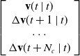 $\left.\left[\begin{array}{c} \mathbf{v}(t\mid t)\\ {\unicode[Arial]{x0394}} \mathbf{v}(t+1\mid t)\\ \cdots \\ {\unicode[Arial]{x0394}} \mathbf{v}(t+N_{c}\mid t) \end{array}\right.\right]$
.
 $\mathbf{H}_{t}$
is the coefficient matrix of control increment
 ${\unicode[Arial]{x0394}} \mathbf{v}$
.
 $\mathbf{e}_{\mathrm{s}}$
is the error between the planned trajectory and reference trajectory.
To solve the local optimal problem of MPC, the IWOA algorithm is used for the rolling optimization of MPC:
 \begin{equation} \begin{array}{c} \min \limits_{{\unicode[Arial]{x0394}} \mathbf{V}(t)}\dfrac{1}{2}\mathbf{X}^{\mathrm{T}}\mathbf{KX}+\mathbf{f}^{\mathrm{T}}\mathbf{X}\\[5pt] \mathrm{s}.\mathrm{t}:\,\mathbf{v}_{\min }\leq \mathbf{v}(t)\leq \mathbf{v}_{\max }\\[5pt] {\unicode[Arial]{x0394}} \mathbf{v}_{\min }\leq {\unicode[Arial]{x0394}} \mathbf{v}(t)\leq {\unicode[Arial]{x0394}} \mathbf{v}_{\max } \end{array} \end{equation}
The conventional parameter adjustment method of WOA is relatively simplistic, leading to slow convergence rates when dealing with complex optimization problems. Moreover, it is difficult to obtain the global optimal solution. To address these issues of WOA, we propose an improved version of WOA that incorporates an elite strategy. By employing the elite strategy at each iteration, high-quality individuals are preserved while inferior ones are eliminated to mitigate the impact of random search on convergence outcomes. Therefore, this improvement not only obtains the global optimal solution but also enhances search efficiency.
The elite can be characterized with global control parameters (GC) and individual state parameters (IS).
 \begin{equation} \begin{array}{c} GC=\left(\dfrac{t_{\max }-t+1}{t_{\max }}\right)^{2}\\[10pt] IS=\dfrac{f(x_{i},t)-f_{\min }}{f_{\max }-f_{\min }} \end{array} \end{equation}
where t is the iteration times,
 $t_{\max }$
represents the maximum iteration,
 $f(x_{i},t)$
represents the fitness values of the present individual at time t, and
 $f_{\min }$
and
 $f_{\max }$
represent the minimum and maximum fitness values, respectively. The global control parameter GC and individual state parameter IS ensure a balance between exploration and exploitation by dynamically adjusting the search range. The search space is controlled by employing GC, which gradually decreases as the number of iterations increases. Individual fitness values are calculated using IS.
The definition of global control parameters for the elite population is as follows:
 \begin{equation} EP=\textit{floor}[(GC-1)\times t_{\max }+TP] \end{equation}
where the floor() function selects the value to the nearest integer, and TP is the total population size. A harmonious equilibrium between exploration and extraction can be attained among elite individuals by selecting the optimal EP based on individual fitness values.
The conventional WOA primarily relies on simple random selection and linear parameter adjustment in the random search phase and employs two fixed strategies for local search during the bubble-net attack phase. In contrast, IWOA integrates these phases into a unified approach to improve the global search capability and local search efficiency through the elite retention mechanism, thereby improving overall optimization performance. The expressions for updating an individual location are as follows [Reference Dai, Yu, Zhang, Zhan and Zheng21]:
 \begin{align} \begin{array}{c} Z(t+1)=Z_{\text{best}}(t)-\chi _{u}\cdot o\cdot \mu _{a}\\[4pt] \mu _{a}=\left| r\cdot Z_{b}(t)-Z(t)\right| \\[4pt] o=2\omega \sigma _{1}-\omega \\[4pt] \omega =2-\frac{2t}{t_{\max }} \end{array} \end{align}
where
 $\chi _{u}$
is the search direction factor indicating the population,
 $Z(t)$
is the position vector of the current individual, and
 $Z_{\text{best}}(t)$
is the optimal position vector of the current individual.
 $r=2\sigma _{2} , \sigma _{1}$
and
 $\sigma _{2}$
are random numbers between [0, 1].
 $\omega$
is a convergence factor that traverses from 2 to 0. If the present fitness is less than the past fitness value, then the
 $\chi _{u}$
value is −1. If the present fitness value is greater than the past fitness value, then the
 $\chi _{u}$
value is 1. Each iteration generates two new individuals to improve the quality of the elite individual:
 \begin{align} \begin{array}{l} Z_{\mathrm{new}1}=Z_{\min }+\sigma (Z_{\max }-Z_{\min })\\[5pt] Z_{\mathrm{new}2}=Z_{\max }+\sigma (Z_{\max }-Z_{\min }) \end{array} \end{align}
where
 $Z_{\min }$
and
 $Z_{\max }$
are the individuals with the lowest and highest fitness values in the population, respectively,
 $\sigma$
is the random number between [0, 1].
To improve search accuracy, the original logarithmic spiral is replaced with an Archimedean spiral. The equation for the bubble-net attack phase is provided as:
 \begin{equation}\begin{aligned} Z(t+1)&=\mu _{b}\cdot \varepsilon \tau \cdot \cos (2\pi \tau )+Z_{b}(t)\\[5pt] \mu _{b}&=\left| r\cdot Z_{\text{best}}(t)-Z(t)\right| \end{aligned} \end{equation}
where
 $\varepsilon$
is the defining constant of the Archimedean helix,
 $\tau$
is a random number in [−1, 1].
The comprehensive model can be formulated as:
 \begin{align} Z\left(t+1\right)=\begin{cases} Z(t+1)=Z_{\text{best}}(t)-\chi _{u}\cdot o\cdot \mu _{a} & \sigma \lt \upsilon \\[4pt] Z(t+1)=\mu _{b}\cdot \varepsilon \tau \cdot \cos (2\pi \tau )+Z_{b}(t) & \sigma \gt \upsilon \end{cases} \end{align}
where
 $\upsilon$
is employed to concurrently achieve the exploration phase (prey encirclement) and the exploitation phase (bubble-netting), and
 $\upsilon$
changes between 1 and 0 as the number of iterations increases.
After the rolling optimization process of IWOA, certain columns indicating the control increment are obtained as:
 \begin{equation} \left.\mathbf{\Delta }\mathbf{V}=\left[\begin{array}{llll} {\unicode[Arial]{x0394}} {\boldsymbol{\nu }}_{z,t}^{\ast } & {\unicode[Arial]{x0394}} {\boldsymbol{\nu }}_{z,t+1}^{\ast } & \cdots & {\unicode[Arial]{x0394}} {\boldsymbol{\nu }_{z,t+{N_{\mathrm{c}}}-1}}^{\ast } \end{array}\right.\right]^{\mathrm{T}} \end{equation}
where
 ${\unicode[Arial]{x0394}} {\boldsymbol{\nu }}_{z,t}^{\ast } , {\unicode[Arial]{x0394}} {\boldsymbol{\nu }}_{z,t+1}^{\ast }$
, …,
 ${\unicode[Arial]{x0394}} {\boldsymbol{\nu }}_{z,t+N_{\mathrm{c}}-1}^{\ast }$
represent the control increment obtained through rolling optimization using IWOA.
The control output can be calculated by
 \begin{equation} \boldsymbol{\nu }_{z}(t)=\boldsymbol{\nu }_{z}(t-1)+{\unicode[Arial]{x0394}} {\boldsymbol{\nu }_{zt}}^{\ast } \end{equation}
The completion of the MPC rolling optimization will result in the generation of a series of motion trajectories, which are defined as:
 \begin{equation} \mathbf{S}^{*}=\left[\begin{array}{llll} \mathbf{s}^{*}(t) & \mathbf{s}^{*}(t+1) & \cdots & \mathbf{s}^{*}(t+N_{c}-1) \end{array}\right]^{\mathrm{T}} \end{equation}
3.3. Optimize trajectories using the two-layer B-spline optimization framework
The combination of APF and IMPC generates a collision-free trajectory for the CDCR in the environment with obstacles. However, the planned trajectory generated by APF-IMPC may lack smoothness, which reduces tracking accuracy and stability of CDCRs and increases the risk of collision with obstacles. Therefore, in order to improve the smoothness of the planned trajectories, a two-layer B-spline optimization framework is employed.
3.3.1. B-spline curves preliminaries
B-splines can generate continuous and differentiable piecewise polynomial curves. The knot values of the B-spline curve serve as the generated points of the trajectory. The formula expressing the B-spline curve is presented as [Reference Webster and Jones27]:
 \begin{equation} \mathbf{b}\!\left(u\right)=\sum\limits_{i=0}^{m}N_{i,p}\left(u\right)\mathbf{p}_{i},{\quad}u_{0}\leq u\leq u_{e} \end{equation}
where
 $N_{i,p}(u)$
represents the basis function of the B-spline curve at knot value u, p stands for the degree of the B-spline curve, and
 $\mathbf{p}_{i}$
denotes control points of the B-spline curve.
According to the Cox-DeBoor recursion, the basic functions of the B-spline curve are as follows:
 \begin{align} \begin{array}{c} N_{i,0}\!\left(u\right)=\begin{cases} 1 & \text{if }u_{i}\lt u\lt u_{i+1}\\[3pt] 0 &\qquad \text{other} \end{cases} \\[15pt] N_{i,p}\!\left(u\right)=\dfrac{u-u_{i}}{u_{i+p}-u_{i}}N_{i,p-1}\!\left(u\right)+\dfrac{u_{i+p+1}-u}{u_{i+p+1}-u_{i+1}}N_{i+1,p-1}\!\left(u\right) \end{array} \end{align}
The kth derivative of
 $N_{i,p}(u)$
can be calculated as:
 \begin{align} {N}_{i,p}^{\left(k\right)}\!\left(u\right)=p\left(\frac{{N}_{i,p-1}^{(k-1)}}{u_{i+p}-u_{i}}-\frac{{N}_{i+1,p-1}^{(k-1)}}{u_{i+p+1}-u_{i+1}}\right) \end{align}
where k = 1, 2, …, p. So, the kth derivation of the B-spline curve can be computed as:
 \begin{equation} \mathbf{b}^{\left(k\right)}\left(u\right)=\sum\limits_{i=0}^{n}{N}_{i,p}^{\left(k\right)}\!\left(u\right)\!\mathbf{p}_{i} \end{equation}
Cubic B-splines are employed to ensure the continuity of velocity and acceleration of the CDCR, while effectively balancing computational efficiency and smoothness constraints [Reference Van Hoek, Ploeg and Nijmeijer28].
By employing quasi-uniform B-splines for approximate processing, the knot vector of B-splines can be expressed as:
 \begin{equation} \mathbf{\psi }=\left\{\underset{p+1}{\underbrace{u_{0},\ldots ,u_{0}}},u_{p+1},\ldots ,u_{n},\underset{p+1}{\underbrace{u_{e},\ldots ,u_{e}}}\right\} \end{equation}
where
 $u_{0}=0$
, the node values at both ends of the node vector have a multiplicity of p + 1.
B-spline needs to sample m + 1 points from the trajectory S
* generated by IMPC. The newly generated m + 1 points are
 $\mathbf{b}_{0},\mathbf{b}_{1},\ldots ,\mathbf{b}_{m}$
. The node values are calculated using spline parameterization and the speed constraint [Reference Piegl and Tiller29]:
 \begin{equation} u_{i+4}-u_{i+3}=\max \frac{\left| \mathbf{s}^{*}(t+i+1)-\mathbf{s}^{*}(t+i)\right| }{v_{\max }}, i=0,1,\ldots ,m-1\!. \end{equation}
B-spline is utilized to improve the smoothness and continuity of the trajectory. There are two methods of B-spline in trajectory processing: interpolation and approximation. When employing the interpolation method, it is imperative for the trajectory to precisely traverse through the designated feature points. It may result in a substantial alteration of curvature at the control points and subsequently induce trajectory instability. In contrast, the approximation rule enables the trajectory to generally approximate the feature points, thereby reducing the likelihood of abrupt changes and oscillations. Although the approximation method may make the trajectory intersect with obstacles, it yields smoother trajectories compared to interpolation.
The smoothness of the B-spline curve is calculated by the following formula:
 \begin{equation} \min O=\eta \sum\limits_{k=0}^{m}\lambda _{k}\left| \mathbf{b}\left(\overline{u}_{k}\right)^{2}-\mathbf{s}_{k}\right| ^{2}+\left(1-\eta \right){\int }_{\overline{u}_{0}}^{\overline{u}_{m}}\left| \frac{\mathrm{d}^{2}\mathbf{b}(u)}{\mathrm{d}u^{2}}\right| ^{2}\mathrm{d}u \end{equation}
where
 $ \eta \epsilon$
[0, 1] is the smoothing parameter, and
 $\lambda _{k}$
is the error measurement weight for the kth segment of the B-spline. The first term is relevant to the distance between the B-spline curve and waypoints. Another term reflects the smoothness penalty. As
 $ \eta $
increases, the weight of the first term in (34) also increases, which makes the B-spline curve approach the locus point. When
 $ \eta $
decreases, the second term in (34) will have a greater weight, resulting in a smoother trajectory.
By substituting (28)–(30) in (34), we can get a new objection function:
 \begin{equation} \left.\min O(\mathbf{P})=\eta \mathrm{tr}[(\mathbf{S}^{*}-\mathbf{NP})^{\mathrm{T}}\mathbf{\chi }(\mathbf{S}^{*}-\mathbf{NP})\right]+(1-\eta )\mathrm{tr}\left[\mathbf{P}^{\mathrm{T}}\Theta _{N}\mathbf{P}\right] \end{equation}
where
 $\mathbf{P}=[\mathbf{p}_{0},\mathbf{p}_{1},\ldots ,\mathbf{p}_{m}]^{T} , \mathbf{S}^{*}=[\begin{array}{llll} \mathbf{s}^{*}(t) & \mathbf{s}^{*}(t+1) & \cdots & \mathbf{s}^{*}(t+N_{c}-1) \end{array}]^{\mathrm{T}} , \mathbf{\chi }=\text{diag}(\lambda _{0},\ldots ,\lambda _{m}) , \{\mathbf{N}\}_{ij}=N_{j,p}(\overline{u}_{i})$
and
 $\{\Theta _{N}\}_{jk}=\int {N}_{j}^{\mathit{'}\mathit{'}}(t){N}_{k}^{\mathit{'}\mathit{'}}(t)\mathrm{d}t$
. By defining the derivative of
 $O(\mathbf{P})=0$
, the control point P can be derived as:
 \begin{equation} \mathbf{P}=\left(\begin{array}{l} \frac{1-\eta }{\eta }\Theta _{N}+\mathbf{N}^{\mathrm{T}}\mathbf{\chi }\mathbf{N} \end{array}\right)^{-1}\mathbf{N}^{\mathrm{T}}\mathbf{\chi }\mathbf{S}^{*} \end{equation}
3.3.2. The two-layer B-spline optimization framework
B-spline enhances the smoothness of the optimized APF-IMPC collision-free trajectory. However, due to the uncontrollable change of curvature between control points in the process of obstacle avoidance, the trajectory will collide with obstacles. Therefore, to improve the smoothness and safety of the APF-IMPC planned trajectory, a two-layer B-spline optimization framework is designed. By implementing this second layer, the proposed framework explicitly overcomes the traditional flaw of B-splines, where the curve breaches minimum clearance limits due to convex hull constraints. The diagram in Figure 4 illustrates the flowchart of the two-layer B-spline.
Flow chart of the two-layer B-spline framework.

The first layer improves the smoothness of the trajectory generated by APF-IMPC. In the environment with fewer obstacles, it can achieve a safe and smooth trajectory.
It should be noted that it is necessary to determine whether it collides with obstacles after optimization. The formula for detecting the collision between the B-spline optimized trajectory and obstacles is as follows:
 \begin{equation} | | \mathbf{b}\left(u\right)-\mathbf{s}_{j,\mathrm{obs}}| | ^{2}\geq l_{\min } \end{equation}
where
 $\mathbf{s}_{j,\mathrm{obs}}$
is the position of the closest obstacle. If the first layer’s optimized trajectory interacts with the obstacle, the second layer is activated.
The second layer is suitable for use in the case of narrow channels and multi-obstacles. The second layer consists of two processes. The first adjustment process modifies the control parameters of the B-spline for the collision segment, making the optimized trajectory closely align with the trajectory generated by APF-IMPC. If the kth segment of the optimized trajectory collides with the obstacle, a significantly large positive integer is assigned to the weight
 $\lambda _{k}$
for measuring segment error, ensuring that the kth B-spline segment moves towards the APF-IMPC trajectory.
The first adjustment process is depicted in Figure 5, where the trajectory produced by APF-IMPC is denoted as a gray line, the B-spline optimization trajectory is depicted by the green line, and the adjusted trajectory is shown in blue. The collision position that occurs between segment
 ${\mathbf{b}(\overline{u}_{i-1})\mathbf{b}(\overline{u}_{i})}$
and the obstacle is marked by the black grid in Figure 5. Here,
 $\mathbf{b}(\overline{u}_{i-1})$
and
 $\mathbf{b}(\overline{u}_{i})$
are the track points before adjustment.
 $\mathbf{b}(u_{i-1})$
and
 $\mathbf{b}(u_{i})$
are the trajectory points generated by the first adjustment process. The trajectory points
 $\mathbf{b}(\overline{u}_{i-1})$
and
 $\mathbf{b}(\overline{u}_{i})$
move towards
 $\mathbf{b}(u_{i-1})$
and
 $\mathbf{b}(u_{i})$
of the APF-IMPC trajectory by assigning weight parameter
 $\lambda _{i-1}=\lambda _{i}=10^{7}$
in the colliding segment.
The first process of the second layer for the B-spline strategy.

The calculation burden of the first adjustment process is small, allowing it to effectively solve the problem of collision with obstacles in most cases. However, when the CDCR comes to narrow passages, the first adjustment process is not sufficient to ensure safety. Therefore, when the collision with the obstacle still occurs after the first adjustment process, the second adjustment process is activated to further avoid collision with the obstacle.
As shown in Figure 6, the gray trajectory illustrates the trajectory generated by APF-IMPC, while the green trajectory represents the trajectory after applying the first layer of optimization. The blue trajectory depicts the trajectory modified by the second adjustment process of the second layer. If the trajectory optimized by B-spline collides with the obstacle at
 ${\mathbf{b}(\overline{u}_{i-1})\mathbf{b}(\overline{u}_{i})}$
, then
 $\mathbf{b}(\overline{u}_{i-1})$
and
 $\mathbf{b}(\overline{u}_{i})$
need to move towards the outside of the obstacle. Since the obstacle avoidance trajectory after B-spline optimization is always curved, we only need to ensure that the two endpoints
 $\mathbf{b}(\overline{u}_{i-1})$
and
 $\mathbf{b}(\overline{u}_{i})$
of the collision section are in the same straight line with the farthest point of the obstacle so as to ensure that the trajectory is collision-free (as shown in the second image of Figure 6).
The second process of the second layer for the B-spline strategy.

Figure 6. Long description
Panel A: A line graph showing the path of a cable-driven continuum robot navigating around obstacles. The x-axis is labeled x(cm) ranging from 0 to 40, and the y-axis is labeled y(cm) ranging from 0 to 40. The path starts at the bottom left corner marked as Start and ends at the top right corner marked as End. The robot’s path is depicted in blue, with a magnified section highlighted. Panel B: A magnified view of the collision segment from Panel A. The graph shows the robot’s path in green and blue lines, with annotations indicating the collision segment, the farthest point of the obstacle, and the adjust distance. The x-axis and y-axis are not explicitly labeled but are consistent with the scale in Panel A.
Therefore, according to the positions of points
 $\mathbf{b}(\overline{u}_{i-1})$
and
 $\mathbf{b}(\overline{u}_{i})$
, a straight line
 $l_{1}$
passing through the two points can be obtained. Move the straight line
 $l_{1}$
in the direction without obstacles until it reaches the farthest point of obstacles. This line is called
 $l_{2}$
. Draw a perpendicular line from
 $\mathbf{b}(\overline{u}_{i})$
to
 $l_{1}$
, and the intersection point between the perpendicular line and
 $l_{2}$
is
 $\mathbf{b}(u_{i})$
. The adjusted distance between
 $\mathbf{b}(\overline{u}_{i})$
and
 $\mathbf{b}(u_{i})$
is denoted as
 ${\unicode[Arial]{x0394}} \mathbf{b}_{i}$
. Similarly, we can obtain
 $\mathbf{b}(u_{i-1})$
and
 ${\unicode[Arial]{x0394}} \mathbf{b}_{i-1}$
. This linear solution can not only ensure the safety of the trajectory but also reduce the computational burden. It should be noted that in practical applications, the vertical distance between line
 $l_{2}$
and the farthest point of the obstacle should be greater than the safe distance.
Next, the optimized collision-free trajectory can be obtained only by the required moving distance of the control point. According to (28), we can obtain
 \begin{align} \left[\begin{array}{c} N_{i,3}\left(\overline{u}_{i}\right)N_{i+1,3}\left(\overline{u}_{i}\right)N_{i+2,3}\left(\overline{u}_{i}\right) \end{array}\right]\left[\begin{array}{c} {\unicode[Arial]{x0394}} {\mathbf{p}}_{i}^{\mathrm{T}}\\[4pt] {\unicode[Arial]{x0394}} {\mathbf{p}}_{i+1}^{\mathrm{T}}\\[4pt] {\unicode[Arial]{x0394}} {\mathbf{p}}_{i+2}^{\mathrm{T}} \end{array}\right]={\unicode[Arial]{x0394}} {\mathbf{b}}_{i}^{\mathrm{T}} \end{align}
where
 ${\unicode[Arial]{x0394}} \mathbf{p}_{i}$
represents the movement distance of the control point. As can be seen from Figure 6, points
 $\mathbf{b}(\overline{u}_{i-1})$
and
 $\mathbf{b}(\overline{u}_{i})$
need to be adjusted at the same time. Therefore, it can be obtained by extending (39):
 \begin{align} \left[\begin{array}{cccc} \begin{array}{c} N_{i-1,3}\left(\overline{u}_{i-\mathrm{1}}\right)\\[4pt] 0 \end{array} &\quad \begin{array}{c} N_{i,3}\left(\overline{u}_{i-\mathrm{1}}\right)\\[4pt] N_{i,3}\left(\overline{u}_{i}\right) \end{array} &\quad \begin{array}{c} N_{i-\mathrm{1},3}\left(\overline{u}_{i-\mathrm{1}}\right)\\[4pt] N_{i+1,3}\left(\overline{u}_{i}\right) \end{array} &\quad \begin{array}{c} 0\\[4pt] N_{i+2,3}\left(\overline{u}_{i}\right) \end{array} \end{array}\right]\left[\begin{array}{c} {\unicode[Arial]{x0394}} {\mathbf{p}}_{i-1}^{\mathrm{T}}\\[4pt] {\unicode[Arial]{x0394}} {\mathbf{p}}_{i}^{\mathrm{T}}\\[4pt] {\unicode[Arial]{x0394}} {\mathbf{p}}_{i+1}^{\mathrm{T}}\\[4pt] {\unicode[Arial]{x0394}} {\mathbf{p}}_{i+2}^{\mathrm{T}} \end{array}\right]=\left[\begin{array}{c} \Delta {\mathbf{b}_{i-1}}^{\mathrm{T}}\\[4pt] \Delta {\mathbf{b}_{i}}^{\mathrm{T}} \end{array}\right] \end{align}
By applying the minimum-length solution method [Reference Fowler and Bartels30], we can get
 \begin{equation} {\unicode[Arial]{x0394}} {\mathbf{P}}_{c}^{\mathrm{T}}={\mathbf{N}}_{cp}^{\mathrm{T}}\left(\mathbf{N}_{cp}{\mathbf{N}}_{cp}^{\mathrm{T}}\right)^{-1}{\unicode[Arial]{x0394}} {\mathbf{B}}_{c}^{\mathrm{T}} \end{equation}
where
 ${\unicode[Arial]{x0394}} {\mathbf{P}}_{c}^{\mathrm{T}}=[\begin{array}{cccc} {\unicode[Arial]{x0394}} {\mathbf{p}}_{i-\mathrm{1}}^{\mathrm{T}} &\,\, {\unicode[Arial]{x0394}} {\mathbf{p}}_{i}^{\mathrm{T}} &\,\, {\unicode[Arial]{x0394}} {\mathbf{p}}_{i+\mathrm{1}}^{\mathrm{T}} &\,\, {\unicode[Arial]{x0394}} {\mathbf{p}}_{i+\mathrm{2}}^{\mathrm{T}} \end{array}]^{\mathrm{T}} , \mathbf{N}_{cp}=\left[\begin{array}{cccc} \begin{array}{c} N_{i-1,3}(\overline{u}_{i-\mathrm{1}})\\ 0 \end{array} &\,\, \begin{array}{c} N_{i,3}(\overline{u}_{i-\mathrm{1}})\\ N_{i,3}(\overline{u}_{i}) \end{array} &\,\, \begin{array}{c} N_{i-\mathrm{1},3}(\overline{u}_{i-\mathrm{1}})\\ N_{i+1,3}(\overline{u}_{i}) \end{array} &\,\, \begin{array}{c} 0\\ N_{i+2,3}(\overline{u}_{i}) \end{array} \end{array}\right] , {\unicode[Arial]{x0394}} {\mathbf{B}}_{c}^{\mathrm{T}}=\left[\begin{array}{c} \Delta {\mathbf{b}_{i-1}}^{\mathrm{T}}\\ \Delta {\mathbf{b}_{i}}^{\mathrm{T}} \end{array} \right]$
. After the adjustment process, a smoother collision-free trajectory can be obtained.
4. Trajectory tracking
IMPC is also further employed to guarantee precise tracking of the planned trajectory.
It is worth noting that while the geometric adjustment in the B-spline framework ensures spatial safety, it may occasionally generate reference points that challenge the joint rotation limits. The incorporation of rigorous kinematic constraints (12), (13), (14), and (15) within this tracking IMPC serves as a critical safeguard, ensuring that the physical execution strictly conforms to the flexible joints’ rotational and bending capacities.
The IMPC algorithm adjusts acceleration iteratively to achieve optimal values, thereby preventing velocity jumps during tracking. In this study, APF is not employed in trajectory tracking for two primary reasons: (1) during the trajectory planning stage, a safe collision-free trajectory has already been generated by APF-IMPC. (2) APF utilized as the penalty term of the objective function will increase computational burden. Therefore, hard constraints are introduced in trajectory tracking to ensure that the distance between the CDCR and obstacles remains greater than the safe distance.
The MPC-based trajectory tracking controller is constructed as follows:
 \begin{align} \begin{array}{c} {\unicode[Arial]{x0394}} {\mathbf{v}}_{tr}^{*}=\underset{{\unicode[Arial]{x0394}} v}{\text{argmin}}W\left({\unicode[Arial]{x0394}} \mathbf{v}_{\mathrm{tr}}\right)\\[6pt] W\left({\unicode[Arial]{x0394}} \mathbf{v}_{\mathrm{tr}}\right)=\sum \limits_{j=1}^{N_{\mathrm{lp}}}\parallel \mathbf{s}\left(k+j| t\right)-\mathbf{b}^{*}\!\left(k+j| t\right){\parallel }_{\mathbf{Q}_{\mathrm{l}}}^{2}+\sum \limits_{j=0}^{N_{\mathrm{lc}}-1}\parallel {\unicode[Arial]{x0394}} \mathbf{v}_{\mathrm{tr}}\left(k+j| t\right){\parallel }_{\mathbf{R}_{\mathrm{l}}}^{2}\\[6pt] \mathrm{s}.\mathrm{t}\colon l(s,s_{obs})\gt l_{min}\\[6pt] \alpha _{\min }\leq \alpha \leq \alpha _{\max }\\[6pt] {\unicode[Arial]{x0394}} \mathbf{v}_{\min }\leq {\unicode[Arial]{x0394}} \mathbf{v}_{\mathrm{tr}}(t)\leq {\unicode[Arial]{x0394}} \mathbf{v}_{\max }\\[6pt] \beta _{\min }\leq \beta \leq \beta _{\max }\\[6pt] \mathbf{s}\in \mathbf{A} \end{array} \end{align}
where
 ${\unicode[Arial]{x0394}} \mathbf{v}_{\mathrm{tr}}$
represents the control increment of the CDCR.
 $N_{\mathrm{lp}}$
and
 $N_{\mathrm{lc}}$
are prediction domains and control domains, respectively.
 $\mathbf{Q}_{\mathrm{l}}$
is the state weighting matrix, and
 $\mathbf{R}_{\mathrm{l}}$
is the control increment weighting matrix. Impose stability constraints:
 \begin{equation} \boldsymbol{| }\boldsymbol{| }\mathbf{s}(k+N_{\mathrm{lp}}| t)-\mathbf{b}^{*}(k+N_{\mathrm{lp}}| t)| {| }_{\mathbf{Q}_{\mathrm{l}}}^{2}=0 \end{equation}
Convert (42) to the objective function form with a constraint:
 \begin{align} \begin{array}{c} \min \limits_{{\unicode[Arial]{x0394}} V(t)}\dfrac{1}{2}{\mathbf{X}_{\mathrm{tr}}}^{\mathrm{T}}\mathbf{K}_{\mathrm{tr}}\mathbf{X}_{\mathrm{tr}}+{\mathbf{f}_{\mathrm{tr}}}^{\mathrm{T}}\mathbf{X}_{\mathrm{tr}}+{\epsilon} ^{2}\rho _{\mathrm{tr}}\\[6pt] \mathrm{s}.\mathrm{t}:\,\mathbf{v}_{\min }\leq \mathbf{v}(t)\leq \mathbf{v}_{\max }\\[6pt] {\unicode[Arial]{x0394}} \mathbf{v}_{\min }\leq {\unicode[Arial]{x0394}} \mathbf{v}_{\mathrm{tr}}(t)\leq {\unicode[Arial]{x0394}} \mathbf{v}_{\max } \end{array} \end{align}
where
 $\mathbf{X}_{\mathrm{tr}}=\left[\begin{array}{c} \Delta \mathbf{V}_{\mathrm{tr}}(t)\\ {\varepsilon} \end{array}\right] , \left.\mathbf{K}_{\mathrm{tr}}=\left[\begin{array}{cc} 2{\mathbf{H}}_{\mathrm{tr}}^{\mathrm{T}}\mathbf{Q}_{\mathrm{l}}\mathbf{H}_{\mathrm{tr}}+\mathbf{R}_{\mathrm{l}} &\quad 0\\ 0 &\quad \rho _{\mathrm{tr}} \end{array}\right.\right] , {\mathbf{f}_{\mathrm{tr}}}^{\mathrm{T}}=\left[\begin{array}{cc} -2{\mathrm{e}}_{\mathrm{str}}^{\mathrm{T}}\mathbf{Q}_{\mathrm{l}}\mathbf{H}_{\mathrm{tr}} &\quad 0 \end{array}\right]$
and
 $\big.{\unicode[Arial]{x0394}} \mathbf{V}_{\mathrm{tr}}\left(t\right)=$
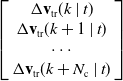 $\left[\begin{array}{c} {\unicode[Arial]{x0394}} \mathbf{v}_{\mathrm{tr}}(k\mid t)\\ {\unicode[Arial]{x0394}} \mathbf{v}_{\mathrm{tr}}(k+1\mid t)\\ \cdots \\ {\unicode[Arial]{x0394}} \mathbf{v}_{\mathrm{tr}}(k+N_{\mathrm{c}}\mid t) \end{array}\big.\right]\!$
.
 $\mathbf{v}(t) , \mathbf{v}_{\min }$
and
 $\mathbf{v}_{\max }$
are the moving speed, minimum moving speed, and maximum moving speed, respectively.
 $\mathbf{H}_{\mathrm{tr}}$
is the coefficient matrix of
 ${\unicode[Arial]{x0394}} \mathbf{v}_{\mathrm{tr}}$
.
 $\mathbf{e}_{\mathrm{str}}$
is the error between the tracking trajectory and the planned trajectory.
In the process of tracking trajectory, IWOA is used to optimize
 ${\unicode[Arial]{x0394}} \mathbf{V}_{\mathrm{tr}}(t)$
to reduce the oscillation phenomenon and tracking error. The IWOA optimization process still uses (19)–(24), which is not detailed here.
After dynamic rolling optimization of IWOA, it can get a series of speed increments.
 \begin{equation} \mathbf{\Delta }{\mathbf{V}_{\mathrm{tr}}}^{\ast }=\left[\!\begin{array}{llll} {\unicode[Arial]{x0394}} {\mathbf{v}_{\mathrm{tr},k}}^{\ast } & {\unicode[Arial]{x0394}} {\mathbf{v}_{\mathrm{tr},k+1}}^{\ast } & \cdots & {\unicode[Arial]{x0394}} {\mathbf{v}_{\mathrm{tr},k+{N_{\mathrm{lc}}}-1}}^{\ast } \end{array}\!\right]^{\mathrm{T}} \end{equation}
where
 ${\unicode[Arial]{x0394}} {\mathbf{v}_{\mathrm{tr},k}}^{\ast } , {\unicode[Arial]{x0394}} {\mathbf{v}_{\mathrm{tr},k+1}}^{\ast }$
, …,
 ${\unicode[Arial]{x0394}} {\mathbf{v}_{\mathrm{tr},k+{N_{\mathrm{lc}}}-1}}^{\ast }$
represents the control increment obtained through the rolling optimization using IWOA.
5. Simulation and discussion
5.1. Simulation platform construction
In this part, the effectiveness of the proposed APF-IMPC and two-layer B-spline optimization framework is verified through a series of simulations using MATLAB/Simulink 2022b.
Parameter setting: To mitigate the occurrence of sudden speed change, the permissible range of joint velocities is set between −0.3 rad/s and 0.3 rad/s. Additionally, the constraints on the bending angle
 $\alpha$
and rotation angle
 $\beta$
are (0, π/2) and (−π, π), respectively.
 $N_{\mathrm{p}}=6, N_{\mathrm{c}}=1$
. The time interval between samples is 0.1 s. The safe distance between the CDCR and obstacles is
 $l_{\min }$
= 4 cm.
5.2. Simulation comparison
Simulations are conducted to evaluate the performance of APF-IMPC and the two-layer B-spline optimization.
-
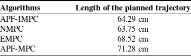
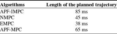
1) Obstacle avoidance effectiveness of APF-IMPC: Figure 7 shows the trajectories of four different algorithms in a multi-obstacle environment. Table I shows the total length of these four trajectories. The effectiveness of the proposed APF-IMPC is comprehensively validated in comparison with NMPC [Reference Lee, Chung, Kim and Kim18], EMPC [Reference Li, Wang, Yang and Zhao19], and APF-MPC [Reference Zhu, Mao, Han, Zhang and Yang20]. In a multiple obstacle scene depicted in Figure 7, the start point is (1, 1, 0) and the endpoint is (40, 40, 25). As illustrated in Figure 7, both NMPC and EMPC encounter collisions with obstacles. This is because EMPC and NMPC only use hard constraints to avoid obstacles, making them easy to collide with obstacles due to infeasible solutions during the planning process. In contrast, both APF-IMPC and APF-IMPC adopt APF as the penalty term of the objective function to avoid the occurrence of infeasible solutions. Moreover, it can be seen from Table I that the planned trajectory length of APF-MPC is larger than that of APF-IMPC. This is because APF-MPC falls into local optima, while APF-IMPC adopts the IWOA algorithm to derive the global optimal solution for MPC. Therefore, APF-IMPC generates a shorter trajectory. To evaluate the computational burden, the average execution time per control step for each algorithm was recorded, as shown in Table II. Although the proposed APF-IMPC exhibits a slightly higher execution time compared to standard NMPC due to the integration of the APF penalty, its average computational time remains well below the 0.4s sampling period used in our physical setup. This indicates that the proposed algorithm efficiently balances trajectory safety, smoothness, and real-time computational feasibility without causing processor overload.
-
2) Two-layer B-spline optimization effectiveness: The second set of simulation experiments verifies the effectiveness of the two-layer B-spline optimization. We validate the first and second layers of the B-spline optimization separately. The first layer uses B-spline to improve the smoothness of the planned trajectory. Figure 8 clearly demonstrates that the first layer of B-spline optimization significantly enhances trajectory smoothness.
Length of the planned trajectory for these four methods.

Table I. Long description
A table comparing the length of planned trajectories for four different algorithms. The table has two columns: Algorithms and Length of the planned trajectory. The first row under Algorithms is APF-IMPC with a trajectory length of 64.29 centimeters. The second row under Algorithms is NMPC with a trajectory length of 63.75 centimeters. The third row under Algorithms is EMPC with a trajectory length of 68.52 centimeters. The fourth row under Algorithms is APF-MPC with a trajectory length of 71.28 centimeters.
Average execution time per control step for different algorithms

Table II. Long description
A table titled Length of the planned trajectory for these four methods. The table has two columns: Algorithms and Length of the planned trajectory. The table contains four rows with the following data: Row 1: Algorithms, Length of the planned trajectory; Row 2: APF-IMPC, 64.29 centimeters; Row 3: NMPC, 63.75 centimeters; Row 4: EMPC, 68.52 centimeters; Row 5: APF-MPC, 71.28 centimeters.
Simulation results of obstacle avoidance in multi-obstacle environments.

As depicted in Figure 9, the use of the first layer may result in collisions. By implementing the first adjustment progress in the second layer of the two-layer B-spline optimization framework, the colliding segments are moved to the original trajectory generated by APF-IMPC. It can be seen from Figure 9 that the collision problem is successfully solved by the first adjustment progress.
Optimization result of the first layer B-spline.

Figure 8. Long description
Panel A: Main view. A 3D line graph displays two trajectories, one in red labeled APF-IMPC generated trajectory and another in blue labeled First layer B-spline optimization. The graph includes green and yellow dots marking the start and end points, respectively. The axes are labeled X (cm), Y (cm), and Z (cm). Panel B: Top view. A 3D line graph from a top perspective shows the same trajectories and markers as Panel A, with axes labeled X (cm) and Y (cm). Panel C: Front view. A 3D line graph from a front perspective shows the same trajectories and markers as Panel A, with axes labeled X (cm) and Z (cm). Panel D: Side view. A 3D line graph from a side perspective shows the same trajectories and markers as Panel A, with axes labeled Y (cm) and Z (cm).
Simulation of the first adjustment progress in the second layer of the two-layer B-spline optimization framework.

In the scene of multi-obstacle and narrow channels, the first adjustment process in the second layer may also cause a collision with obstacles. As shown in Figure 10, if the first progress of the second layer for the two-layer B-spline optimization framework is still unable to separate the trajectory from the obstacles, then the second adjustment progress is implemented to move the trajectory point of the collision section to the side without obstacles, ensuring the safety of the optimized trajectory.
Simulation of the second adjustment progress in the second layer of the two-layer B-spline optimization framework.

Figure 10. Long description
Panel A: A 3D plot showing the overall trajectory planning process. The plot includes a start point at coordinates (10, 10, 0) and an end point at coordinates (50, 40, 20). The trajectory is divided into three layers: the first layer B-spline optimization shown in green, the second layer first adjustment progress in blue, and the second layer second adjustment progress in magenta. The original trajectory is depicted in gray. Various obstacles are represented as blue and cyan cubes. Panel B: A partial top view of the trajectory planning process, highlighting the adjustments made in the second layer. The adjustments are indicated by arrows labeled with Δb_i and Δb_i’ showing the changes in trajectory to avoid obstacles.
Through the above simulations, it can be verified that the two-layer B-spline optimization framework improves trajectory smoothness while ensuring safe obstacle avoidance.
6. Experiment results
The obstacle avoidance performance of the APF-IMPC nested B-spline optimization framework, NMPC [Reference Lee, Chung, Kim and Kim18], EMPC [Reference Li, Wang, Yang and Zhao19], and APF-MPC [Reference Zhu, Mao, Han, Zhang and Yang20] in a multi-obstacle environment is compared through experiments. As shown in Figure 11, the posture sensor GY-95T and the ultrasonic sensor are positioned at the end of the CDCR to measure its position and distance from obstacles, respectively. Four TBS-K30 servos are arranged at the top of the CDCR. The sampling period is 0.4 s. The experimental sampling period was set to 0.4 s to accommodate the mechanical response time of the cable-driven system. This lag primarily arises from the necessity to tension the driving cables and the complex synchronization required among multiple actuators before a posture change is executed.
6.1. Obstacle avoidance effectiveness
Figure 12 shows the obstacle avoidance process of APF-IMPC, NMPC, EMPC, and APF-MPC. In this comparative experiment, to ensure consistency, all algorithms adopt the two-layer B-spline optimization framework. As depicted in Figure 12 (a) and Figure 12 (d), APF-IMPC and APF-MPC demonstrate a safe obstacle avoidance capability. On the contrary, it can be seen from Figure 12 (b) that the trajectory of the NMPC collides with a pink obstacle at the marked position of the blue circle. Similarly, in Figure 12 (c), the trajectory controlled by EMPC collides with a yellow obstacle at the marked position of the blue circle. The reason is that NMPC and EMPC only depend on hard constraints, which may lead to infeasible solutions. In contrast, both APF-IMPC and APF-IMPC adopt APF as the penalty term of the objective function to solve these problems.
Experimental setup of the CDCR.

O-shaped collision-free trajectory in a multi-obstacle environment. (a) APF-IMPC. (b) NMPC. (c) EMPC. (d) APF-MPC.

Figure 12. Long description
Panel A: A series of photos showing the APF-IMPC algorithm in action. The images depict a robotic arm navigating through a multi-obstacle environment. The path of the robotic arm is marked with a red line, starting from a point labeled Start and ending at a point labeled End. The obstacles are represented by colored blocks. Panel B: A series of photos showing the NMPC algorithm in action. Similar to Panel A, the images depict a robotic arm navigating through a multi-obstacle environment. The path of the robotic arm is marked with a red line, starting from a point labeled Start and ending at a point labeled End. A collision point is marked with a blue circle.
However, APF-MPC suffers from the jitter problem, as indicated by the two positions marked with purple circles in Figure 12 (d). On the contrary, there is no jitter in the tracking trajectory of APF-IMPC in Figure 12 (a). This is because the APF-MPC algorithm is easy to get stuck in local optima. In contrast, the designed IWOA algorithm adopted in APF-IMPC can help the control system avoid local optima and obtain the global optimal solution.
To quantitatively evaluate the stability of the trajectory tracking, the positional errors (e x, e y, and e z) between the end effector and the desired trajectory are recorded. As depicted in Figure 13, the tracking errors along the x, y, and z axes are consistently constrained within a small bounded range. Notably, the error curves exhibit smooth transitions without high-frequency oscillations or abrupt spikes, even during aggressive obstacle avoidance maneuvers. These evaluation indicators firmly demonstrate the superior stability and anti-jitter capability of the proposed APF-IMPC tracking controller.
Tracking error between end effector position and desired position.

Figure 13. Long description
Panel A: Three line graphs depict x-direction error over time for four trajectory planning algorithms: APF-IMPC, NMPC, EMPC, and APF-MPC. The x-axis represents time in seconds, and the y-axis represents error in centimeters. Each graph shows the error trends for the respective algorithm. Panel B: Three line graphs depict y-direction error over time for the same algorithms. The x-axis represents time in seconds, and the y-axis represents error in centimeters. Each graph shows the error trends for the respective algorithm. Panel C: Three line graphs depict z-direction error over time for the same algorithms. The x-axis represents time in seconds, and the y-axis represents error in centimeters. Each graph shows the error trends for the respective algorithm.
Therefore, it can be seen from the experiment that APF-IMPC can effectively generate a safe and feasible trajectory compared to NMPC and EMPC, as well as ensuring high-precision trajectory tracking compared to APF-MPC.
6.2. The effectiveness of B-spline optimization framework
In this experiment, the number of obstacles is increased to test the performance of the two-layer B-spline optimization framework. In Figure 14, the green line represents the planned trajectory generated by the traditional B-spline optimization algorithm. The red line represents the planned trajectory using the two-layer B-spline optimization framework, and the blue dotted line represents the original trajectory without optimization.
The planned trajectory by the two algorithms.

It can be clearly seen from Figure 14 that the trajectory becomes smoother after B-spline optimization. However, two collisions occurred at the blue circle mark when using the traditional B-spline algorithm. The reason is that the traditional B-spline optimization algorithm may cause collision with obstacles after changing the original trajectory. On the contrary, when the two-layer B-spline optimization framework encounters the risk of collision with obstacles after improving trajectory smoothness, it will activate the adjustment strategy of the second layer to modify the trajectory to the collision-free area. Therefore, the trajectory of the two-layer B-spline optimization framework does not collide with obstacles. It demonstrates that the proposed APF-IMPC nested two-layer B-spline optimization framework can effectively reduce the risk of motion mutation and collisions in multi-obstacle environments while improving trajectory smoothness.
7. Conclusions
This paper proposes an APF-IMPC nested two-layer B-spline optimization framework to achieve safe and efficient obstacle avoidance for the CDCR in a multi-obstacle environment. Adopting APF as the objective function penalty term to further ensure the safety of generated trajectories. In addition, an IWOA is introduced to avoid the local optimal trap of MPC. The proposed two-level B-spline optimization framework enhances the smoothness of the planned trajectory. Simulation and experiment results demonstrate that the proposed algorithm enables the CDCR to safely and smoothly avoid obstacles in multi-obstacle environments while ensuring high-precision trajectory tracking. Although the IWOA-based IMPC effectively mitigates local optima, the current framework has several limitations that define our future work. First, the elite retention strategy will be upgraded with self-adaptive mechanisms for highly dense environments. Second, an event-triggered localized APF will be investigated to enhance robustness against sudden boundary proximity. Third, future work will consider the adaptive scaling of repulsive field parameters to better accommodate irregular physical obstacles. Finally, formalizing the theoretical convergence proofs to explicitly account for physical imperfections–such as data transmission delays and the persistent position drift caused by thermal expansion during long-duration operations–will be critical. Integrating a disturbance observer into the MPC to compensate for these slow-varying thermo-mechanical dynamics will be our next immediate focus.
Author contribution
This article was written by Shishuai Zhao. Qi Chen and Yanan Qin reviewed and helped revise the content.
Financial support
This work was supported by the National Natural Science Foundation of China under grants 52471336, 52127813, and 52431012.
Conflicts of interest
The authors declare no conflicts of interest exist.