2 Formulation: two dimensions

The flow velocity is written $\boldsymbol{u}=(u(x,z,t),0,w(x,z,t))$ and, adopting the standard assumptions of shallow-water theory (see e.g. Stoker Reference Stoker1957), we make the leading-order approximation that

(2.1) $$\begin{eqnarray}\displaystyle u(x,z,t)\approx U(x,t), & & \displaystyle\end{eqnarray}$$

and

(2.2) $$\begin{eqnarray}\displaystyle w(x,z,t)\approx (z/h(x)+1)\unicode[STIX]{x1D701}_{t}(x,t)+(zh^{\prime }(x)/h(x))U(x,t). & & \displaystyle\end{eqnarray}$$

This choice of $w$ ensures that the kinematic (no-flow) condition on the bed $z=-h(x)$ , expressed by

(2.3) $$\begin{eqnarray}\displaystyle h^{\prime }(x)u(x,-h(x),t)+w(x,-h(x),t)=0, & & \displaystyle\end{eqnarray}$$

is satisfied exactly. On the surface $z=\unicode[STIX]{x1D701}(x,t)$ the linearised kinematic condition

(2.4) $$\begin{eqnarray}\displaystyle w(x,0,t)=\unicode[STIX]{x1D701}_{t}(x,t), & & \displaystyle\end{eqnarray}$$

holds. The linear profile (2.2) was anticipated by Stoker (Reference Stoker1957) and adopted by Peregrine (Reference Peregrine1967).

We apply continuity $u_{x}+w_{z}=0$ in a depth-averaged sense of

(2.5) $$\begin{eqnarray}\displaystyle [w(x,z,t)]_{-h(x)}^{0}=-\int _{-h(x)}^{0}u_{x}(x,z,t)\,\text{d}z. & & \displaystyle\end{eqnarray}$$

After substitution from (2.1) and use of the kinematic equations on the bed and the surface, (2.3) and (2.4), we arrive at

(2.6) $$\begin{eqnarray}\displaystyle \unicode[STIX]{x1D701}_{t}=-(hU)_{x}, & & \displaystyle\end{eqnarray}$$

a result that does not require the definition of $w$ as expressed in (2.2). In passing, we note that the use of (2.6) in (2.2) results in a simplified version of (2.2), namely

(2.7) $$\begin{eqnarray}\displaystyle w\approx \unicode[STIX]{x1D701}_{t}-zU_{x}, & & \displaystyle\end{eqnarray}$$

which is less intuitive than the form originally adopted, although it is clearer to see from (2.7) that $u_{x}+w_{z}=0$ is satisfied pointwise throughout the fluid.

The vertical component of the (linearised) momentum equation is

(2.8a,b ) $$\begin{eqnarray}\displaystyle \unicode[STIX]{x1D70C}w_{t}=-p_{z}-\unicode[STIX]{x1D70C}g,\quad -h(x)<z<0, & & \displaystyle\end{eqnarray}$$

where $\unicode[STIX]{x1D70C}$ is the fluid density and $p(x,z,t)$ is the pressure. In the derivation of the standard SWE, the term $\unicode[STIX]{x1D70C}w_{t}$ does not contribute at leading order and is therefore neglected. Following arguments given in the introduction herein, we retain the $\unicode[STIX]{x1D70C}w_{t}$ term and, after using (2.2) in (2.8), we find

(2.9) $$\begin{eqnarray}\displaystyle p_{z}=-\unicode[STIX]{x1D70C}g-\unicode[STIX]{x1D70C}(z/h(x)+1)\unicode[STIX]{x1D701}_{tt}-\unicode[STIX]{x1D70C}(zh^{\prime }(x)/h(x))U_{t}. & & \displaystyle\end{eqnarray}$$

(We could use (2.7) in place of (2.2), but there is no significant algebraic benefit in what follows.) Integrating (to leading order) and enforcing $p=p_{a}$ , atmospheric pressure, on $z=\unicode[STIX]{x1D701}(x,t)$ gives

(2.10) $$\begin{eqnarray}\displaystyle p(x,z,t)=p_{a}+\unicode[STIX]{x1D70C}g(\unicode[STIX]{x1D701}-z)-\unicode[STIX]{x1D70C}\left({\displaystyle \frac{z^{2}}{2h(x)}}+z\right)\unicode[STIX]{x1D701}_{tt}-\unicode[STIX]{x1D70C}{\displaystyle \frac{z^{2}h^{\prime }(x)}{2h(x)}}U_{t}. & & \displaystyle\end{eqnarray}$$

This expression will now be used in the horizontal component of the momentum equation, which, like the continuity equation, is applied in a vertically averaged sense. Thus

(2.11) $$\begin{eqnarray}\displaystyle Q_{t} & = & \displaystyle -{\displaystyle \frac{1}{\unicode[STIX]{x1D70C}}}\int _{-h(x)}^{0}p_{x}\,\text{d}z\nonumber\\ \displaystyle & = & \displaystyle -gh\unicode[STIX]{x1D701}_{x}-\frac{1}{3}h^{2}\unicode[STIX]{x1D701}_{ttx}-\frac{1}{6}hh^{\prime }\unicode[STIX]{x1D701}_{tt}+\frac{1}{6}h^{2}h^{\prime }U_{tx}+\frac{1}{6}(h^{2}h^{\prime \prime }-h{h^{\prime }}^{2})U_{t}\end{eqnarray}$$

expressed in terms of $Q(x,t)$ , the depth-averaged horizontal flux, and includes contributions beyond leading-order terms in the expansion in the bed shallowness parameter on the left-hand side of (2.11) but can be made equal to its leading-order value $hU(x,t)$ elsewhere. Henceforth the dependence of $h$ upon $x$ is dropped for clarity. The relation $hU_{tx}=(hU_{t})_{x}-h^{\prime }U_{t}$ is used to express, via (2.6), the above in the form

(2.12) $$\begin{eqnarray}\displaystyle \left\{1+{\textstyle \frac{1}{3}}{h^{\prime }}^{2}-{\textstyle \frac{1}{6}}hh^{\prime \prime }\right\}Q_{t}=-gh\unicode[STIX]{x1D701}_{x}-{\textstyle \frac{1}{3}}h^{2}\unicode[STIX]{x1D701}_{ttx}-{\textstyle \frac{1}{3}}hh^{\prime }\unicode[STIX]{x1D701}_{tt}. & & \displaystyle\end{eqnarray}$$

Dividing by the bracketed term on the left-hand side and differentiating with respect to $x$ allows us to eliminate $Q$ using (2.6) to obtain

(2.13) $$\begin{eqnarray}\displaystyle \unicode[STIX]{x1D701}_{tt}={\displaystyle \frac{\unicode[STIX]{x2202}}{\unicode[STIX]{x2202}x}}\left({\displaystyle \frac{h\left(g\unicode[STIX]{x1D701}+{\textstyle \frac{1}{3}}h\unicode[STIX]{x1D701}_{tt}\right)_{x}}{1+{\textstyle \frac{1}{3}}{h^{\prime }}^{2}-{\textstyle \frac{1}{6}}hh^{\prime \prime }}}\right), & & \displaystyle\end{eqnarray}$$

and this is the time-dependent extended SWE, though not exactly aligned to the form expressed in (1.1). Assuming a time-harmonic dependence by writing $\unicode[STIX]{x1D701}(x,t)=\text{Re}\{\unicode[STIX]{x1D702}(x)\text{e}^{-\text{i}\unicode[STIX]{x1D714}t}\}$ results in

(2.14) $$\begin{eqnarray}\displaystyle \left({\displaystyle \frac{h\left(\left(1-{\textstyle \frac{1}{3}}Kh\right)\unicode[STIX]{x1D702}\right)^{\prime }}{1+{\textstyle \frac{1}{3}}{h^{\prime }}^{2}-{\textstyle \frac{1}{6}}hh^{\prime \prime }}}\right)^{\prime }+K\unicode[STIX]{x1D702}=0, & & \displaystyle\end{eqnarray}$$

where $K=\unicode[STIX]{x1D714}^{2}/g$ , and writing $\unicode[STIX]{x1D713}(x)=(1-{\textstyle \frac{1}{3}}Kh(x))\unicode[STIX]{x1D702}(x)$ allows us to express the SWE in the same form as the original version (1.2), as

(2.15) $$\begin{eqnarray}\displaystyle ({\hat{h}}\unicode[STIX]{x1D713}^{\prime })^{\prime }+\hat{K}\unicode[STIX]{x1D713}=0, & & \displaystyle\end{eqnarray}$$

where

(2.16) $$\begin{eqnarray}\displaystyle \left.\begin{array}{@{}l@{}}{\hat{h}}(x)=h(x)/\left(1+{\textstyle \frac{1}{3}}{h^{\prime }}^{2}(x)-{\textstyle \frac{1}{6}}h(x)h^{\prime \prime }(x)\right)\!,\\ \hat{K}(x)=K/\left(1-{\textstyle \frac{1}{3}}Kh(x)\right),\end{array}\right\} & & \displaystyle\end{eqnarray}$$

are scaled versions of $h$ and $K$ .

Instead of eliminating $Q$ in favour of $\unicode[STIX]{x1D702}$ , we can return to (2.12), differentiate with respect to $t$ and use (2.6) to find that

(2.17) $$\begin{eqnarray}\displaystyle \left\{\!1+{\textstyle \frac{1}{3}}{h^{\prime }}^{2}-{\textstyle \frac{1}{6}}hh^{\prime \prime }\right\}Q_{tt}=h\left(gQ_{x}+{\textstyle \frac{1}{3}}hQ_{ttx}\right)_{x}, & & \displaystyle\end{eqnarray}$$

with $\unicode[STIX]{x1D701}_{t}=-Q_{x}$ , is an alternative to (2.13). If $Q(x,t)=\text{Re}\{q(x)\text{e}^{-\text{i}\unicode[STIX]{x1D714}t}\}$ then (2.17) reduces to

(2.18) $$\begin{eqnarray}\displaystyle (\hat{K}^{-1}q^{\prime })^{\prime }+{\hat{h}}^{-1}q=0, & & \displaystyle\end{eqnarray}$$

with $\unicode[STIX]{x1D702}=-(\text{i}/\unicode[STIX]{x1D714})q^{\prime }$ , which becomes an alternative to (2.15) that retains the structure of (1.2).

Whilst (2.15) and (2.18) provide equally valid descriptions of wave scattering by the bed, $h(x)$ , the latter version is able to cope with discontinuities in bed slopes since we can use the differential equation to determine the jump condition

(2.19) $$\begin{eqnarray}\displaystyle [q^{\prime }(x)]_{c^{-}}^{c^{+}}={\textstyle \frac{1}{6}}\hat{K}(c)q(c)[h^{\prime }(x)]_{c^{-}}^{c^{+}}, & & \displaystyle\end{eqnarray}$$

where $x=c$ is a point of discontinuity in $h^{\prime }(x)$ . The relationship between $q$ and the surface elevation implies that $\unicode[STIX]{x1D702}(x)$ is discontinuous whenever $h^{\prime }(x)$ is. This seems odd but is simply an outcome of the underlying assumptions adopted in this approximation. We remark that, in the standard SWE, $\unicode[STIX]{x1D702}^{\prime }(x)$ is discontinuous at corners in the bed for similar reasons.

A transformed version of the SWE (2.18) can be developed by introducing the scaling

(2.20) $$\begin{eqnarray}\displaystyle q(x)=\unicode[STIX]{x1D711}(x)/\sqrt{1-{\textstyle \frac{1}{3}}Kh}, & & \displaystyle\end{eqnarray}$$

which, after substituting into (2.18) and working through the algebra, results in

(2.21) $$\begin{eqnarray}\displaystyle \unicode[STIX]{x1D711}^{\prime \prime }(x)+\left\{\hat{K}\left(1+{\textstyle \frac{1}{3}}v(h){h^{\prime }}^{2}\right)/h\right\}\unicode[STIX]{x1D711}(x)=0, & & \displaystyle\end{eqnarray}$$

where $v(h)=1+{\textstyle \frac{1}{12}}\hat{K}h\approx 1$ for $Kh\ll 1$ . This form of the SWE does not contain terms proportional to $h^{\prime \prime }(x)$ , and thus $\unicode[STIX]{x1D711}(x)$ is continuous even when $h^{\prime }$ is discontinuous. The free surface is reconstructed in terms of $\unicode[STIX]{x1D711}(x)$ with

(2.22) $$\begin{eqnarray}\displaystyle \unicode[STIX]{x1D702}(x)={\displaystyle \frac{(-\text{i}/\unicode[STIX]{x1D714})}{\sqrt{1-{\textstyle \frac{1}{3}}Kh}}}(\unicode[STIX]{x1D711}^{\prime }(x)+{\textstyle \frac{1}{6}}\hat{K}h^{\prime }\unicode[STIX]{x1D711}(x)), & & \displaystyle\end{eqnarray}$$

and discontinuities in $\unicode[STIX]{x1D702}(x)$ at points of discontinuity of $h^{\prime }(x)$ are now clearly manifested by the second term. If we further let $\unicode[STIX]{x1D6FA}(x)=\unicode[STIX]{x1D711}^{\prime }(x)$ , then (2.21) implies that $\unicode[STIX]{x1D6FA}^{\prime }(x)=-\{\hat{K}(1+{\textstyle \frac{1}{3}}v(h){h^{\prime }}^{2})/h\}\unicode[STIX]{x1D711}(x)$ and it follows that

(2.23) $$\begin{eqnarray}\displaystyle (\hat{{\hat{h}}}\unicode[STIX]{x1D6FA}^{\prime })^{\prime }+K\unicode[STIX]{x1D6FA}=0, & & \displaystyle\end{eqnarray}$$

where

(2.24) $$\begin{eqnarray}\displaystyle \hat{{\hat{h}}}(x)=h(x){\displaystyle \frac{\left(1-{\textstyle \frac{1}{3}}Kh(x)\right)}{\left(1+{\textstyle \frac{1}{3}}v(h){h^{\prime }}^{2}(x)\right)}}, & & \displaystyle\end{eqnarray}$$

is once more aligned with (1.2) and becomes the alternative to (2.15) without discontinuities in the dependent variable at points of discontinuity in the bed. The transformed version of (2.22) is

(2.25) $$\begin{eqnarray}\displaystyle \unicode[STIX]{x1D702}(x)={\displaystyle \frac{(-\text{i}/\unicode[STIX]{x1D714})}{\sqrt{1-{\textstyle \frac{1}{3}}Kh}}}\left(\unicode[STIX]{x1D6FA}(x)-{\displaystyle \frac{{\textstyle \frac{1}{6}}hh^{\prime }}{1+{\textstyle \frac{1}{3}}v(h){h^{\prime }}^{2}}}\unicode[STIX]{x1D6FA}^{\prime }(x)\right). & & \displaystyle\end{eqnarray}$$

In practice $\hat{{\hat{h}}}(x)$ as defined by (2.24) can be used in place of $h(x)$ in (1.2) to furnish results for the extended SWE for all continuous $h(x)$ .

For waves propagating over a flat bed, $h(x)=h_{0}$ a constant, say, any one of equations (2.15), (2.18), (2.21) or (2.23) can be used to show that solutions are given by $\unicode[STIX]{x1D702}(x)=\text{e}^{\pm \text{i}k_{0}x}$ , where $k_{0}$ satisfies $k_{0}^{2}h_{0}^{2}=Kh_{0}/(1-{\textstyle \frac{1}{3}}Kh_{0})$ . This agrees to second order in $Kh_{0}$ with the expansion of the exact dispersion relation for waves over constant depth $h_{0}$ , namely $K=k_{0}\tanh k_{0}h_{0}$ , which is readily found to be $k_{0}^{2}h_{0}^{2}\approx Kh_{0}(1+{\textstyle \frac{1}{3}}Kh_{0}+O(Kh_{0})^{2})$ for $Kh_{0}\ll 1$ . In contrast, solutions of (1.2) are given in terms of a wavenumber satisfying $k_{0}^{2}h_{0}^{2}=Kh_{0}$ , which only captures the leading-order behaviour. Thus, the extended SWE includes weak dispersion not captured within the original SWE.

D. Porter (personal communication, 2019) has independently derived a version of (2.21) that agrees at leading order in the bed slope $h^{\prime }$ and its three-dimensional analogue seen later in (3.18) but with $\hat{K}=K$ , $v(h)=1$ , by considering the long-wavelength limit of the CMSE, originally due to Kim & Bai (Reference Kim and Bai2004) and Toledo & Agnon (Reference Toledo and Agnon2010).

The long-wavelength limit of Porter (D. Porter, personal communication, 2019) fails to capture the factors $1-{\textstyle \frac{1}{3}}Kh$ responsible for the weakly dispersive effect in (2.21) and (2.22) or the lower-order corrective term $v(h)$ . It is supposed that this mismatch is a consequence of the fundamentally different initial starting points that have been adopted in the modelling, Porter’s (D. Porter, personal communication, 2019) derivation evolving from a variational formulation of the problem.

We also note the relationship of the equations we have derived to the work of Ehrenmark (Reference Ehrenmark2005), who considered the effect of wave propagation over a constant plane slope on the local dispersion relation. In that work a modified dispersion relation was proposed, which replaced the local depth $h(x)$ by an effective depth $h(x)/(1+{\textstyle \frac{1}{3}}{h^{\prime }}^{2}(x)+O({h^{\prime }}^{4}))$ , which agrees at leading order with the definition both of ${\hat{h}}(x)$ in (2.16) and of $\hat{{\hat{h}}}(x)$ in (2.24).

3 Three dimensions

Now the bed is given by $z=-h(x,y)$ and the free surface by $z=\unicode[STIX]{x1D701}(x,y,t)$ . One can easily show that the analogue of the continuity equation (2.6) is

(3.1) $$\begin{eqnarray}\displaystyle \unicode[STIX]{x1D701}_{t}=-\unicode[STIX]{x1D735}\boldsymbol{\cdot }(h\boldsymbol{U}), & & \displaystyle\end{eqnarray}$$

where $\boldsymbol{U}=(U(x,y,t),V(x,y,t))$ and $\unicode[STIX]{x1D735}=(\unicode[STIX]{x2202}_{x},\unicode[STIX]{x2202}_{y})$ following an assumption that the flow velocity takes the form

(3.2) $$\begin{eqnarray}\displaystyle \boldsymbol{u}\approx (\boldsymbol{U},(z/h+1)\unicode[STIX]{x1D701}_{t}+(z/h)\unicode[STIX]{x1D735}h\boldsymbol{\cdot }\boldsymbol{U}), & & \displaystyle\end{eqnarray}$$

and satisfies $w=\unicode[STIX]{x1D701}_{t}$ on $z=0$ and $w+\unicode[STIX]{x1D735}h\boldsymbol{\cdot }\boldsymbol{U}=0$ on $z=-h(x,y)$ .

Following the derivation in § 2, with the momentum equation in the horizontal plane written $\unicode[STIX]{x1D70C}\boldsymbol{U}_{t}=-\unicode[STIX]{x1D735}p$ , leads to the equation for the depth-integrated flux $\boldsymbol{Q}$ (equal to $h\boldsymbol{U}$ at leading order)

(3.3) $$\begin{eqnarray}\displaystyle \boldsymbol{Q}_{t}=-gh\unicode[STIX]{x1D735}\unicode[STIX]{x1D701}-{\textstyle \frac{1}{3}}h^{2}\unicode[STIX]{x1D735}\unicode[STIX]{x1D701}_{tt}-{\textstyle \frac{1}{6}}h\{\unicode[STIX]{x1D701}_{tt}+(\unicode[STIX]{x1D735}h\boldsymbol{\cdot }(\boldsymbol{Q}_{t}/h))\}\unicode[STIX]{x1D735}h+{\textstyle \frac{1}{6}}h^{2}\unicode[STIX]{x1D735}(\unicode[STIX]{x1D735}h\boldsymbol{\cdot }(\boldsymbol{Q}_{t}/h)), & & \displaystyle\end{eqnarray}$$

and this can be rearranged in the form

(3.4) $$\begin{eqnarray}\displaystyle \boldsymbol{Q}_{t}=-gh\unicode[STIX]{x1D735}\unicode[STIX]{x1D701}-{\displaystyle \frac{1}{3}}h^{2}\unicode[STIX]{x1D735}\unicode[STIX]{x1D701}_{tt}-{\displaystyle \frac{h\unicode[STIX]{x1D701}_{tt}}{6}}\unicode[STIX]{x1D735}h-{\displaystyle \frac{1}{3}}h(\unicode[STIX]{x1D735}h\boldsymbol{\cdot }(\boldsymbol{Q}_{t}/h))\unicode[STIX]{x1D735}h+{\displaystyle \frac{1}{6}}h\unicode[STIX]{x1D735}(\unicode[STIX]{x1D735}h\boldsymbol{\cdot }\boldsymbol{Q}_{t}). & & \displaystyle\end{eqnarray}$$

With some more work, this equation can be reduced to

(3.5) $$\begin{eqnarray}\displaystyle \boldsymbol{Q}_{t}+{\textstyle \frac{1}{3}}(\unicode[STIX]{x1D735}h\boldsymbol{\cdot }\boldsymbol{Q}_{t})\unicode[STIX]{x1D735}h-{\textstyle \frac{1}{6}}h\unicode[STIX]{x1D65D}^{\prime \prime }\boldsymbol{Q}_{t}+{\textstyle \frac{1}{6}}h\unicode[STIX]{x1D63F}\boldsymbol{Q}_{t}=-\unicode[STIX]{x1D735}\left(g\unicode[STIX]{x1D701}+{\textstyle \frac{1}{3}}h\unicode[STIX]{x1D701}_{tt}\right), & & \displaystyle\end{eqnarray}$$

where $\unicode[STIX]{x1D65D}^{\prime \prime }$ represents the $2\times 2$ Hessian matrix of $h(x,y)$ which multiplies vector $\boldsymbol{Q}_{t}$ , and

(3.6) $$\begin{eqnarray}\displaystyle \unicode[STIX]{x1D63F}=\left(\begin{array}{@{}cc@{}}0 & \boldsymbol{t}\boldsymbol{\cdot }\unicode[STIX]{x1D735}\\ -\boldsymbol{ t}\boldsymbol{\cdot }\unicode[STIX]{x1D735} & 0\end{array}\right), & & \displaystyle\end{eqnarray}$$

is an antisymmetric differential operator where $\boldsymbol{t}=(-h_{y},h_{x})$ is directed along level curves of $h(x,y)$ .

Introducing $\unicode[STIX]{x1D644}$ as the $2\times 2$ identity matrix and writing

(3.7) $$\begin{eqnarray}\displaystyle {\unicode[STIX]{x1D65D}^{\prime }}^{2}=(\unicode[STIX]{x1D735}h)(\unicode[STIX]{x1D735}h)^{\text{T}}=\left(\begin{array}{@{}cc@{}}h_{x}^{2} & h_{x}h_{y}\\ h_{x}h_{y} & h_{y}^{2}\end{array}\right), & & \displaystyle\end{eqnarray}$$

(notation aligned to the two-dimensional setting) we may rearrange (3.6) as

(3.8) $$\begin{eqnarray}\displaystyle \left\{\unicode[STIX]{x1D644}+{\textstyle \frac{1}{3}}{\unicode[STIX]{x1D65D}^{\prime }}^{2}-{\textstyle \frac{1}{6}}h\unicode[STIX]{x1D65D}^{\prime \prime }+{\textstyle \frac{1}{6}}h\unicode[STIX]{x1D63F}\right\}\boldsymbol{Q}_{t}=-h\unicode[STIX]{x1D735}\left(g\unicode[STIX]{x1D701}+{\textstyle \frac{1}{3}}h\unicode[STIX]{x1D701}_{tt}\right). & & \displaystyle\end{eqnarray}$$

As it stands we are not able to eliminate $\boldsymbol{Q}$ in favour of $\unicode[STIX]{x1D701}$ as we did in the two-dimensional case. If we decide to eliminate $\unicode[STIX]{x1D701}$ in favour of $\boldsymbol{Q}$ by taking the time derivative of (3.8) and substituting from (3.1), we find

(3.9) $$\begin{eqnarray}\displaystyle h^{-1}\left\{\unicode[STIX]{x1D644}+{\textstyle \frac{1}{3}}{\unicode[STIX]{x1D65D}^{\prime }}^{2}-{\textstyle \frac{1}{6}}h\unicode[STIX]{x1D65D}^{\prime \prime }+{\textstyle \frac{1}{6}}h\unicode[STIX]{x1D63F}\right\}\boldsymbol{Q}_{tt}=\unicode[STIX]{x1D735}\left(g\unicode[STIX]{x1D735}\boldsymbol{\cdot }\boldsymbol{Q}+{\textstyle \frac{1}{3}}h\unicode[STIX]{x1D735}\boldsymbol{\cdot }\boldsymbol{Q}_{tt}\right)\!, & & \displaystyle\end{eqnarray}$$

where $\unicode[STIX]{x1D701}_{t}=-\unicode[STIX]{x1D735}\boldsymbol{\cdot }\boldsymbol{Q}$ . Thus, in the time domain, it appears that we can do no better than the vector governing equation (3.9). With $\boldsymbol{Q}(x,y,t)=\text{Re}\{\boldsymbol{q}(x,y)\text{e}^{-\text{i}\unicode[STIX]{x1D714}t}\}$ we have

(3.10) $$\begin{eqnarray}\displaystyle \unicode[STIX]{x1D735}(\hat{K}^{-1}\unicode[STIX]{x1D735}\boldsymbol{\cdot }\boldsymbol{q})+h^{-1}\left\{\unicode[STIX]{x1D644}+{\textstyle \frac{1}{3}}{\unicode[STIX]{x1D65D}^{\prime }}^{2}-{\textstyle \frac{1}{6}}h\unicode[STIX]{x1D65D}^{\prime \prime }+{\textstyle \frac{1}{6}}h\unicode[STIX]{x1D63F}\right\}\boldsymbol{q}=0, & & \displaystyle\end{eqnarray}$$

with $\unicode[STIX]{x1D702}(x,y)=-(\text{i}/\unicode[STIX]{x1D714})\unicode[STIX]{x1D735}\boldsymbol{\cdot }\boldsymbol{q}$ , and

(3.11) $$\begin{eqnarray}\displaystyle \hat{K}(x,y)=K/\left(1-{\textstyle \frac{1}{3}}Kh(x,y)\right), & & \displaystyle\end{eqnarray}$$

is the extension of (2.16) to functions of two variables.

Consider that the bed $h(x,y)$ has a discontinuity in gradients at points $\boldsymbol{c}$ along the curve $\unicode[STIX]{x1D6E4}\in \mathbb{R}^{2}$ having unit normal $\hat{\boldsymbol{n}}$ directed from $\unicode[STIX]{x1D6E4}^{-}$ to $\unicode[STIX]{x1D6E4}^{+}$ . Then (3.10) shows that the jump conditions for points $\boldsymbol{c}$ on $\unicode[STIX]{x1D6E4}$ take the form

(3.12) $$\begin{eqnarray}\displaystyle [\unicode[STIX]{x1D735}\boldsymbol{\cdot }\boldsymbol{q}]_{\unicode[STIX]{x1D6E4}^{-}}^{\unicode[STIX]{x1D6E4}^{+}}={\textstyle \frac{1}{6}}\hat{K}(\boldsymbol{c})\hat{\boldsymbol{n}}\boldsymbol{\cdot }\boldsymbol{q}(\boldsymbol{c})[\hat{\boldsymbol{n}}\boldsymbol{\cdot }\unicode[STIX]{x1D735}h]_{\unicode[STIX]{x1D6E4}^{-}}^{\unicode[STIX]{x1D6E4}^{+}}. & & \displaystyle\end{eqnarray}$$

Thus far, the three-dimensional case has failed to furnish a scalar equation in either the time or the frequency domains and the vector equations for $\boldsymbol{Q}$ and $\boldsymbol{q}$ are complicated by the appearance of the operator $\unicode[STIX]{x1D63F}$ , not present in the two-dimensional case.

However, as in the two-dimensional case, we can make further useful progress by introducing the scaling

(3.13) $$\begin{eqnarray}\displaystyle \boldsymbol{q}(x,y)=\unicode[STIX]{x1D753}(x,y)/\sqrt{1-{\textstyle \frac{1}{3}}Kh}, & & \displaystyle\end{eqnarray}$$

into (3.10). After considerable, but routine, algebra we arrive at

(3.14) $$\begin{eqnarray}\displaystyle \unicode[STIX]{x1D735}(\unicode[STIX]{x1D735}\boldsymbol{\cdot }\unicode[STIX]{x1D753})+(\hat{K}/h)\left\{\unicode[STIX]{x1D644}+{\textstyle \frac{1}{3}}v(h){\unicode[STIX]{x1D65D}^{\prime }}^{2}\right\}\unicode[STIX]{x1D753}=0, & & \displaystyle\end{eqnarray}$$

and $v(h)=1+{\textstyle \frac{1}{12}}\hat{K}h$ is the same factor as derived in the previous section. Now the function $\unicode[STIX]{x1D753}(x,y)$ is continuous even at discontinuities in the gradients of the bed. The free surface is found to be related to $\unicode[STIX]{x1D753}$ by

(3.15) $$\begin{eqnarray}\displaystyle \unicode[STIX]{x1D702}(x,y)={\displaystyle \frac{(-\text{i}/\unicode[STIX]{x1D714})}{\sqrt{1-{\textstyle \frac{1}{3}}Kh}}}(\unicode[STIX]{x1D735}\boldsymbol{\cdot }\unicode[STIX]{x1D753}+{\textstyle \frac{1}{6}}\hat{K}\unicode[STIX]{x1D735}h\boldsymbol{\cdot }\unicode[STIX]{x1D753}). & & \displaystyle\end{eqnarray}$$

The simplified vector equation (3.14) also provides the platform for a scalar version of the extended SWE in three dimensions since writing $\unicode[STIX]{x1D6FA}(x,y)=\unicode[STIX]{x1D735}\boldsymbol{\cdot }\unicode[STIX]{x1D753}$ means that (3.14) becomes

(3.16) $$\begin{eqnarray}\displaystyle \unicode[STIX]{x1D753}=-(\hat{\hat{\unicode[STIX]{x1D65D}}}/K)\unicode[STIX]{x1D735}\unicode[STIX]{x1D6FA}, & & \displaystyle\end{eqnarray}$$

where

(3.17) $$\begin{eqnarray}\displaystyle \hat{\hat{\unicode[STIX]{x1D65D}}}(x,y) & = & \displaystyle h(x,y)\left(1-{\textstyle \frac{1}{3}}Kh\right)\left(\unicode[STIX]{x1D644}+{\textstyle \frac{1}{3}}v(h){\unicode[STIX]{x1D65D}^{\prime }}^{2}\right)^{-1}\nonumber\\ \displaystyle & = & \displaystyle h(x,y)\left(1-{\displaystyle \frac{1}{3}}Kh\right)\left(\unicode[STIX]{x1D644}-{\displaystyle \frac{v(h)}{(3+v(h)|\unicode[STIX]{x1D735}h|^{2})}}{\unicode[STIX]{x1D65D}^{\prime }}^{2}\right).\end{eqnarray}$$

Thus, we arrive at

(3.18) $$\begin{eqnarray}\displaystyle \unicode[STIX]{x1D735}\boldsymbol{\cdot }(\hat{\hat{\unicode[STIX]{x1D65D}}}\unicode[STIX]{x1D735}\unicode[STIX]{x1D6FA})+K\unicode[STIX]{x1D6FA}=0, & & \displaystyle\end{eqnarray}$$

as the scalar version of the extended SWE for $\unicode[STIX]{x1D6FA}(x,y)$ presented in the form (1.2) but with the scalar function $h(x,y)$ replaced by the $2\times 2$ matrix $\hat{\hat{\unicode[STIX]{x1D65D}}}(x,y)$ . The surface elevation is reconstructed from $\unicode[STIX]{x1D6FA}$ using

(3.19) $$\begin{eqnarray}\displaystyle \unicode[STIX]{x1D702}(x,y)={\displaystyle \frac{(-\text{i}/\unicode[STIX]{x1D714})}{\sqrt{1-{\textstyle \frac{1}{3}}Kh}}}(\unicode[STIX]{x1D6FA}-{\textstyle \frac{1}{6}}h\unicode[STIX]{x1D735}h\boldsymbol{\cdot }((\unicode[STIX]{x1D644}+{\textstyle \frac{1}{3}}v(h){\unicode[STIX]{x1D65D}^{\prime }}^{2})^{-1}\unicode[STIX]{x1D735}\unicode[STIX]{x1D6FA})), & & \displaystyle\end{eqnarray}$$

where discontinuities in $\unicode[STIX]{x1D735}h$ can be seen to produce corresponding discontinuities in  $\unicode[STIX]{x1D702}$ .

The development from $\boldsymbol{q}$ through to $\unicode[STIX]{x1D6FA}$ follows closely the work of Toledo & Agnon (Reference Toledo and Agnon2010) (the variable $\unicode[STIX]{x1D6FA}$ is used in recognition of this), who developed a scalar CMSE from the original vector equation derived by Kim & Bai (Reference Kim and Bai2004). The CMSE, given in (A 3), is a depth-averaged model in which the depth variation in the fluid is approximated in such a way as to satisfy the bed condition exactly, and formally requires shallow bed gradients but is not restricted to long wavelengths. The result of taking the limit $Kh\rightarrow 0$ in Toledo & Agnon’s (Reference Toledo and Agnon2010) scalar equation is (A 5), which coincides with (3.18) provided approximations to leading order in $Kh$ are made to $\hat{K}\approx K$ and $v(h)\approx 1$ . In other words, there are differences between (A 5) and (3.18) in higher-order terms in $Kh$ . This limit is also noted by Porter (D. Porter, personal communication, 2019), who derived the same scalar CMSE but using a more general variational principle than that used by Kim & Bai (Reference Kim and Bai2004).

Both the scalar equation (3.18) and the vector equation (3.14) representing three-dimensional scattering demonstrate anisotropy. That is, waves taken to propagate in different directions at the same point $(x,y)$ in space will, in general, travel with different speeds relating to the gradients of the bed in those directions. This might come as a surprise to some readers but is possibly known to others, not least since it can be inferred from Toledo & Agnon’s (Reference Toledo and Agnon2010) work. What is most certainly useful is the explicit dependence of those wave speeds on the function $h(x,y)$ , which can be inferred from (3.17). Indeed, the real benefit of using the extended SWE in place of the CMSE is the simple explicit dependence on $h$ in the former compared to the complex implicit dependence on $h$ in the latter – see (A 3).

4 Examples

4.1 Numerical solutions: two-dimensional wave scattering

In the case of reflection and transmission of waves of frequency $\unicode[STIX]{x1D714}$ incident from $x=-\infty$ over a finite region of variable two-dimensional bathymetry between two flat semi-infinite sections, numerical solutions of any of the versions of the SWE derived in § 2 are easy to compute. We shall outline the method applied to the version given by (2.23) for the variable $\unicode[STIX]{x1D6FA}(x)$ , which does not require special treatment at discontinuities in the bed. Assume that for $x<0$ , $h(x)=h_{0}$ and for $x>L$ , $h(x)=h_{L}$ and $h(x)$ is smooth. Then, in $x<0$ ,

(4.1) $$\begin{eqnarray}\displaystyle \unicode[STIX]{x1D6FA}(x)=\text{e}^{\text{i}k_{0}x}+R\text{e}^{-\text{i}k_{0}x}, & & \displaystyle\end{eqnarray}$$

and, in $x>L$ ,

(4.2) $$\begin{eqnarray}\displaystyle \unicode[STIX]{x1D6FA}(x)=T\text{e}^{\text{i}k_{L}x}, & & \displaystyle\end{eqnarray}$$

where $k_{0}h_{0}=\sqrt{Kh_{0}/(1-{\textstyle \frac{1}{3}}Kh_{0})}$ and $k_{L}h_{L}=\sqrt{Kh_{L}/(1-{\textstyle \frac{1}{3}}Kh_{L})}$ , and $R$ and $T$ represent reflection and transmission coefficients. In $0<x<L$ the solution is determined by (2.23). Matching solutions across the two boundaries and elementary manipulation of the algebra that results shows us that $R$ and $T$ can be obtained from

(4.3) $$\begin{eqnarray}\displaystyle \left(\begin{array}{@{}c@{}}R\\ T\end{array}\right)=\left(\begin{array}{@{}cc@{}}\text{i}(K/k_{0})p_{2}(1)-p_{1}(1) & \text{e}^{\text{i}k_{L}L}\\ \text{i}(K/k_{0})q_{2}(1)-q_{1}(1) & \text{i}(K/k_{L})\text{e}^{\text{i}k_{L}L}\end{array}\right)^{-1}\left(\begin{array}{@{}c@{}}\text{i}(K/k_{0})p_{2}(1)+p_{1}(1)\\ \text{i}(K/k_{0})q_{2}(1)+q_{1}(1)\end{array}\right), & & \displaystyle\end{eqnarray}$$

where $p_{i}(1)$ and $q_{i}(1)$ are determined from solving the coupled first-order differential equations

(4.4a,b ) $$\begin{eqnarray}\displaystyle p_{i}^{\prime }(\unicode[STIX]{x1D709})=Lq_{i}(\unicode[STIX]{x1D709})/\hat{{\hat{h}}}(L\unicode[STIX]{x1D709}),\quad q_{i}^{\prime }(\unicode[STIX]{x1D709})=-KLp_{i}(\unicode[STIX]{x1D709}),\quad 0<\unicode[STIX]{x1D709}<1, & & \displaystyle\end{eqnarray}$$

for $i=1,2$ subject to initial conditions $p_{1}(0)=1$ , $q_{1}(0)=0$ , $p_{2}(0)=0$ and $q_{2}(0)=1$ . On account of the scaling used to define the free surface in (2.25), the transmission coefficient associated with free surface amplitudes requires scaling by the factor $\sqrt{1-{\textstyle \frac{1}{3}}Kh_{L}}/\sqrt{1-{\textstyle \frac{1}{3}}Kh_{0}}$ .

The standard SWE uses the same scheme but with $\hat{{\hat{h}}}$ replaced by $h$ and the definitions of $k_{0}$ and $k_{L}$ replaced by $k_{0}=\sqrt{K/h_{0}}$ and $k_{L}=\sqrt{K/h_{L}}$ . The additional scaling of the transmission coefficient referred to above is not necessary.

4.2 The Booij problem

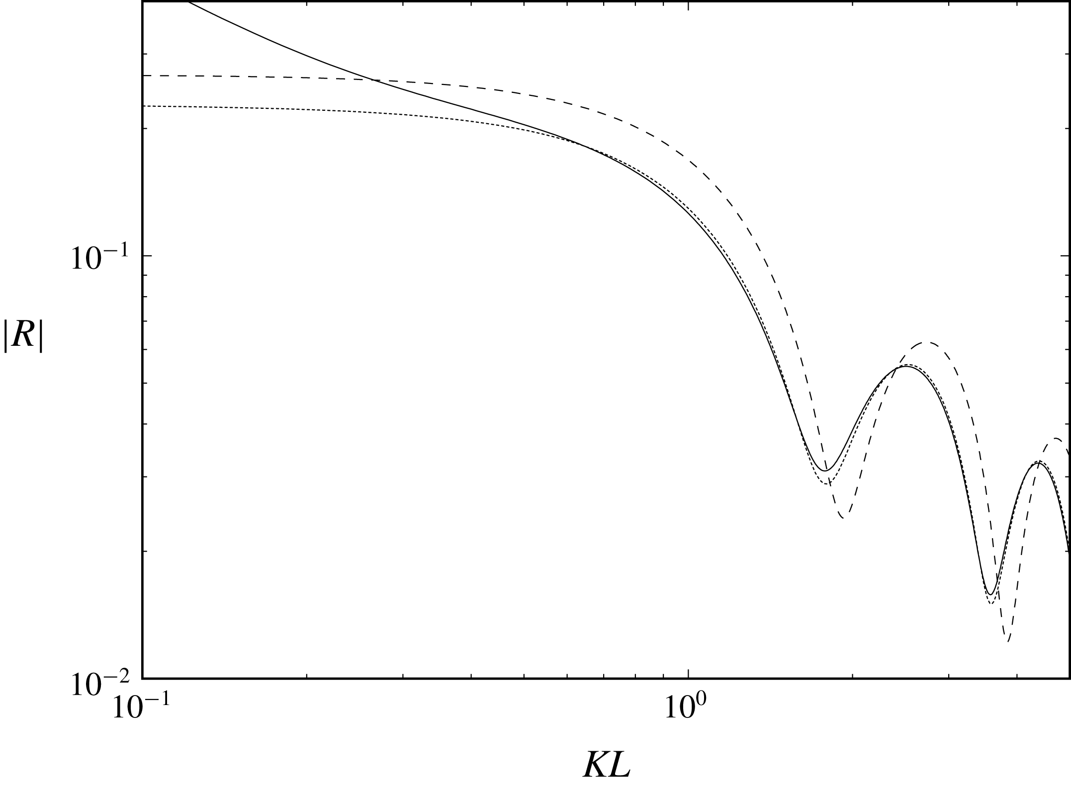
For historical reasons, the Booij problem (Booij Reference Booij1983) has become a standard test case for assessing two-dimensional scattering approximations. A linear slope connects the depth $h_{0}$ to $h_{L}$ over $0<x<L$ and the particular set of results Booij generated are taken for $h_{L}/h_{0}=1/3$ and $Kh_{0}=0.6$ , and $|R|$ is plotted as a function of $KL$ . Since $Kh_{0}$ is fixed and not especially small and the horizontal axis effectively measures steepness of slope, this is not such an enlightening test of the SWE. Indeed, we see in figure 1 that the extended SWE fails compared to the exact results as $KL\rightarrow 0$ and the slope approaches vertical. Neither the standard nor the extended SWE is designed to operate in this regime, and it is simply good fortune that the standard SWE stands as an acceptable approximation up to the point of a vertical step. Instead, the extended SWE fails due to the presence of the ${h^{\prime }}^{2}$ in the denominator of ${\hat{h}}$ or $\hat{{\hat{h}}}$ , which drives the ‘effective depth’ to zero as $KL\rightarrow 0$ and hence the reflection coefficient tends to unity. For smaller gradients (larger values of $KL$ ) below $45^{\circ }$ , figure 1 shows that the extended SWE outperforms the standard SWE by a significant margin, and results are in excellent agreement with the accurate computations based on full linear theory (using the method of Porter & Porter (Reference Porter and Porter2000)). Figure 1 is very similar both qualitatively and quantitatively to figure 8 of Ehrenmark (Reference Ehrenmark2005) and the explanation for this is connected to the discussion at the end of § 2.

Figure 1.

Modulus of reflection coefficient against $KL$ at $Kh_{0}=0.6$ , $h_{L}/h_{0}=1/3$ (the Booij problem): full linear theory (dotted), standard SWE (dashed), extended SWE (solid).

Figure 2.

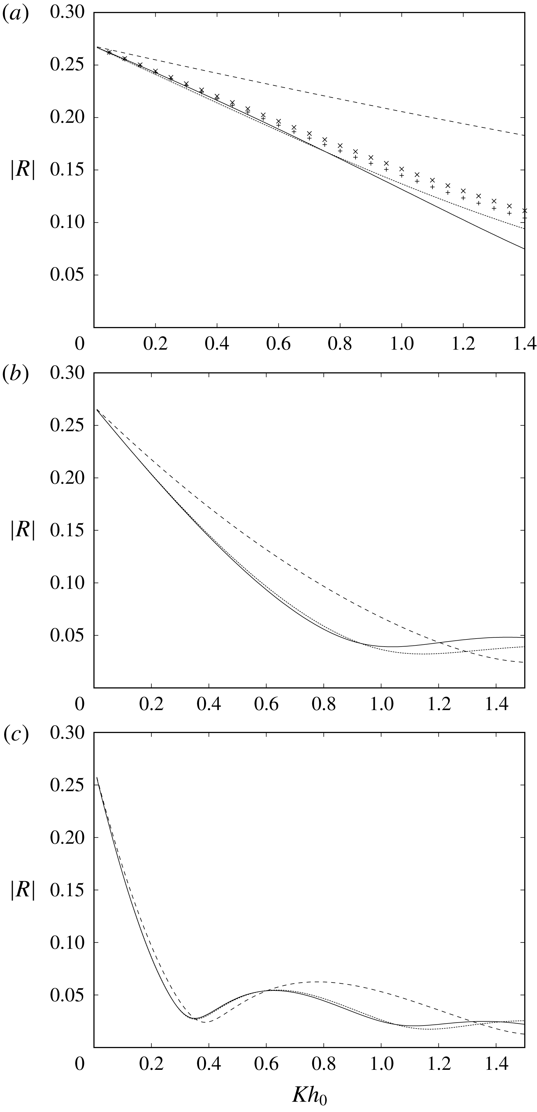
Modulus of reflection coefficient against $Kh_{0}$ for a linear ramp with $h_{L}/h_{0}=1/3$ and $h_{0}/L=1,1/2,~1/4$ in (a–c): full linear theory (dotted), standard SWE (dashed), extended SWE (solid). Results in (a): $+$ , from the CMSE; $\times$ , from the MMSE.

More informative results are shown in figure 2. These are again for a linear slope, but the slope angle is fixed by fixing values of $h_{L}/h_{0}$ and $h_{0}/L$ in each plot and the frequency of incident waves varies from the long-wavelength limit $Kh_{0}\rightarrow 0$ to shorter waves for increasing $Kh_{0}$ . There is a quite remarkable improvement both in the relative performance of the extended SWE over the standard version and in the range of values of $Kh_{0}$ over which good agreement with the exact result is maintained. The standard SWE provides closer agreement for shallower gradients, as might be expected, and the extended SWE works well up to slopes close to $45^{\circ }$ , although the agreement falls away rapidly for steeper slopes (as figure 1 has already shown).

Figure 2(a) also provides, for comparison, results obtained using the scalar CMSE and the modified mild-slope equation (MMSE), given in appendix A. For values of $Kh_{0}>1.4$ , the CMSE and MMSE become increasingly accurate, whilst the extended SWE diverges from the exact results. The extended SWE is arguably the best fit to the exact results for $Kh<1$ . Similar conclusions can be drawn in figure 2(b,c), though data from CMSE and MMSE simulations have not been added to these plots as they are almost indistinguishable from the exact results over the range of values of $Kh_{0}$ plotted.

4.3 Roseau’s solution

Roseau (Reference Roseau1976) provides the only exact solution for waves propagating over a non-constant bathymetry. Thus we have

(4.5) $$\begin{eqnarray}\displaystyle |R|=\left|{\displaystyle \frac{\sinh [(k_{0}h_{0}-k_{L}h_{L})/\unicode[STIX]{x1D6FD}]}{\sinh [(k_{0}h_{0}+k_{L}h_{L})/\unicode[STIX]{x1D6FD}]}}\right|, & & \displaystyle\end{eqnarray}$$

and $\unicode[STIX]{x1D6FD}\in (0,1)$ is a shoaling parameter where the bed is given parametrically as $z(\unicode[STIX]{x1D709})=-h(x(\unicode[STIX]{x1D709}))$ with

(4.6) $$\begin{eqnarray}\displaystyle & \displaystyle x(\unicode[STIX]{x1D709})/h_{0}=\unicode[STIX]{x1D709}-(2\unicode[STIX]{x03C0}\unicode[STIX]{x1D6FD})^{-1}(1-h_{L}/h_{0})\ln (1+\text{e}^{2\unicode[STIX]{x1D6FD}\unicode[STIX]{x03C0}\unicode[STIX]{x1D709}}+2\text{e}^{\unicode[STIX]{x1D6FD}\unicode[STIX]{x03C0}\unicode[STIX]{x1D709}}\cos (\unicode[STIX]{x1D6FD}\unicode[STIX]{x03C0})), & \displaystyle\end{eqnarray}$$

(4.7) $$\begin{eqnarray}\displaystyle & \displaystyle z(\unicode[STIX]{x1D709})/h_{0}=-1+(\unicode[STIX]{x03C0}\unicode[STIX]{x1D6FD})^{-1}(1-h_{L}/h_{0})\tan ^{-1}\{\sin (\unicode[STIX]{x1D6FD}\unicode[STIX]{x03C0})/(\text{e}^{-\unicode[STIX]{x1D6FD}\unicode[STIX]{x03C0}\unicode[STIX]{x1D709}}+\cos (\unicode[STIX]{x1D6FD}\unicode[STIX]{x03C0}))\}. & \displaystyle\end{eqnarray}$$

Then $h^{\prime }(x(\unicode[STIX]{x1D709}))=-z^{\prime }(\unicode[STIX]{x1D709})/x^{\prime }(\unicode[STIX]{x1D709})$ and $h^{\prime \prime }(x(\unicode[STIX]{x1D709}))=-(z^{\prime \prime }(\unicode[STIX]{x1D709})x^{\prime }(\unicode[STIX]{x1D709})-z^{\prime }(\unicode[STIX]{x1D709})x^{\prime \prime }(\unicode[STIX]{x1D709}))/(x^{\prime }(\unicode[STIX]{x1D709}))^{3}$ .

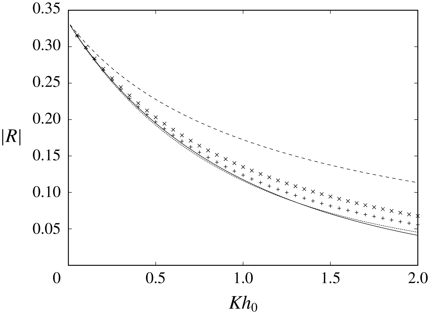
In figure 3 exact results computed from (4.5), where $k_{L}$ and $k_{0}$ are defined by $K=k_{L}\tanh k_{L}h_{L}=k_{0}\tanh k_{0}h_{0}$ , are compared with the new and standard SWE for a shoaling parameter $\unicode[STIX]{x1D6FD}=0.5$ , which gives a maximum gradient of $0.75$ along the profile (see Porter & Porter (Reference Porter and Porter2006) for an illustration of the bed shape). The results demonstrate similar characteristics to those previously considered for the linear slope but without the oscillations due to multiple interference effects caused by the corners at the ends of the transition between the two depths.

Following figure 2(a) we have added results from the CMSE and the MMSE to figure 3 for comparison and we can draw similar conclusions here regarding the accuracy of the extended SWE compared to those models for sufficiently low values of $Kh_{0}$ .

Figure 3.

Modulus of reflection coefficient against $Kh_{0}$ for the Roseau problem with $h_{L}/h_{0}=0.25$ , $\unicode[STIX]{x1D6FD}=0.5$ : full linear theory (dotted), standard SWE (dashed), extended SWE (solid). Also shown are results: $+$  from the CMSE; $\times$  from the MMSE.