INTRODUCTION
Mastitis still remains the most frequent and costly disease in the dairy industry, in terms of economics and animal welfare (Kramer et al. Reference Kramer, Cavero, Stamer and Krieter2009). Early detection and intervention against mastitis reduces veterinary fees, losses in milk yield (MY) and milk quality, and increases the cure rate of the infected animals (Milner et al. Reference Milner, Page and Hillerton1997). With growing herd sizes and the introduction of robotic milking, the classical detection method of visual observation has become more difficult and time consuming. Thus, there is a need to support the farmer's own observations by improved and automated detection of diseases (de Mol et al. Reference De Mol, Kroeze, Achten, Maatje and Rossing1997).
In manufacturing industries as well as agricultural science, several quality variables may be controlled simultaneously. In industrial process control, multivariate quality control charts are most appropriate for such situations. In the case of agricultural science and disease detection in particular, a large number of false positive (FP) alerts coupled with high error rates hinder the application in practice (de Vries & Reneau Reference De Vries and Reneau2010; Miekley et al. Reference Miekley, Traulsen and Krieter2012). In fact, traditional multivariate control charts such as Hoteling's T 2 control charts and multivariate cumulative sum (CUSUM) or exponentially weighted moving average (EWMA) control charts require that quality characteristics follow a multivariate normal distribution (Montgomery Reference Montgomery2009). However, this may not be reasonable in many real-life applications, where the process distribution is unknown (Ben-Hur et al. Reference Ben-Hur, Ong, Sonnenburg, Schölkopf and Rätsch2008). Machine learning, a sub-discipline in the field of artificial intelligence, focuses on algorithms capable of learning and/or adapting their structure (e.g. parameters) based on a set of observed data, with adaptation done by optimizing over an objective or cost function. Machine learning and statistical pattern recognition have been the subject of tremendous interest in the biomedical community because they offer promise for improving the sensitivity and/or specificity of the detection and diagnosis of disease, while at the same time increasing objectivity of the decision-making process (Sajda Reference Sajda2006). Much of the original excitement for the application of machine learning to biomedicine originated from the development of artificial neural networks (ANNs), which were often proclaimed to be ‘loosely’ modelled on computation in the brain. Cavero et al. (Reference Cavero, Tölle, Henze, Buxadé and Krieter2008) applied neural networks to monitor udder health. The problem with ANNs, however, is the difficulty in understanding how such networks construct the desired function and how to interpret the results. Such methods are thus often used as a ‘black box’, with the ANN producing a mapping from input (e.g. medical data) to output (e.g. diagnosis) but without a clear understanding of the underlying function (Sajda Reference Sajda2006).
In an attempt to overcome these difficulties with neural networks, another area in machine learning research has received considerable attention. Support vector machines (SVMs) have demonstrated highly competitive performance in numerous real-world applications such as medical diagnosis, bioinformatics, face recognition, image processing and text mining, thus establishing it as one of the most popular, state-of-the-art tools for knowledge discovery and data mining (Olson & Delen Reference Olson and Delen2008).
Therefore, the aim of the current study was to analyse the applicability of SVMs as a monitoring system for the early detection of mastitis based on practically recorded farm data.
MATERIALS AND METHODS
Data
Data used were recorded on the Karkendamm dairy research farm (Kiel, Germany) between January 2010 and December 2011. During this period, data from 215 cows in their first 200 days in milk (DIM) were available (79 178 milkings). Given mastitis is a disease of the early stage of lactation (Chuganda et al. Reference Chuganda, Friggens, Rasmussen and Larsen2006), only the first 200 DIM were used. Medical treatments of mastitis were documented continuously by veterinarians and farm staff. Different mastitis categories (e.g. Staphylococcus areus or Escherichia coli mastitis) were identified. Due to the low number of diseased cows within these categories, they were combined into ‘cases of mastitis’. These cases were defined as the target characteristic to be distinguished from the healthy observation in the data.
Milking took place in a rotary milking parlour manufactured by GEA Farm Technologies and cows were milked twice daily. Milk yield (MY) and milk electrical conductivity (MEC) of the composite milk were measured using the Metatron P21 milk meter (GEA Farm Technologies) at every milking.
Besides MY and MEC per milking, further input variables (indicator variables) were included successively into the SVM. The combination of input variables with the best results is presented in the following section. The 5-day moving average for the MEC and MY of the morning (mo) and evening (ev) milkings for each cow were calculated, respectively, accounting for cow individuality. The deviations in the actual measured observation from the latest moving average value of each cow were then calculated (dev_MY_mo, dev_MY_ev, dev_MEC_mo, dev_MEC_ev). Increasing deviations from a moving average of each cow were considered as a sign of mastitis, as were augmentations in standard deviation. These were used to determine the 5-day moving standard deviation for the parameters (std_MY_mo, std_MY_ev, std_MEC_mo, std_MEC_ev) of the morning and evening milkings. To provide more detail in the general lactation curve, weeks in lactation (weeks) were divided into 15 classes (Chuganda et al. Reference Chuganda, Friggens, Rasmussen and Larsen2006). The observations collected within the first 8 weeks of lactation were grouped into weekly intervals. Data from weeks 9–16 were grouped into 2-week periods, and data taken later than 17 weeks after calving were grouped into 4-week periods (Hagnestam-Nielsen et al. Reference Hagnestam-Nielsen, Emanuelson, Berglund and Strandberg2009). According to Steeneveld et al. (Reference Steeneveld, Van Der Gaag, Barkema and Hogeveen2009), the month of each observation (January=month 1 to December=month 12) and the cow-specific factor of its own individual mastitis history are also valuable sources of information. The amount of mastitis cases during the observation period of each cow, referred to as history (history=0: no mastitis case before/at all), was up to three cases during the cow's first 200 DIM. The following input variables were used to generate one SVMs model: MEC (one for morning and one for evening milkings), MY (one for morning and one for evening milkings), dev_MEC_mo, dev_MEC_ev, dev_MY_mo, dev_MY_ev, std_MEC_mo, std_MEC_ev, std_MY_mo, std_MY_ev, week, month, history.
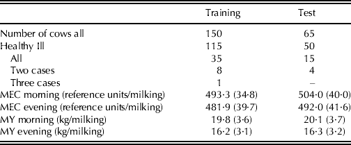
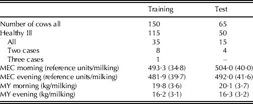
Application of an SVM necessitates the division of data into training and test datasets. Hence, two-thirds of healthy animals and two-thirds of the animals with a disease during the observation period (Wang et al. Reference Wang, Li, Grzymala-Busse, Miao, Skowron and Yao2008) were randomly selected to build the training dataset (Table 1). The remaining one-third in the healthy and diseased dataset were analysed in the test dataset. Descriptive statistical information on the measured traits MY and MEC for the training and test datasets are shown in Table 1.
Number of all, healthy and ill cows as well as the mean (s.d. in parenthesis) of the measured variables milk electrical conductivity (MEC) and milk yield (MY) for training and test datasets
Mastitis definition
Mastitis was defined as disease blocks, i.e. uninterrupted sequences of ‘days of disease’ (Cavero et al. Reference Cavero, Tölle, Henze, Buxadé and Krieter2008; Kramer et al. Reference Kramer, Cavero, Stamer and Krieter2009). The treatments served as a basis for these disease blocks and the different definitions varied solely on the sequence length of the blocks. As the focus of the current study was on early disease detection, only the days before a treatment were included in a disease block (Kramer et al. Reference Kramer, Cavero, Stamer and Krieter2009). If at least one alarm was generated by the monitoring system within the block, it was considered as detected.
Cows were selected for veterinary treatment by the farm staff based on observable signs of mastitis, primarily during milking or during other stable work. Two variants of mastitis definition were used in the current study:
 $$\eqalign{& {\rm Mastitis} + {\rm 3}:\;{\rm treatment}\;{\rm performed}\; {\rm including}\cr & \quad {\rm 3}\;{\rm days}\;{\rm before}\;{\rm the}\;{\rm treatment}} $$
 $$\eqalign{& {\rm Mastitis} + {\rm 4}:\;{\rm treatment}\;{\rm performed} \; {\rm including} \cr & \quad {\rm 4}\;{\rm days}\;{\rm before}\;{\rm the}\;{\rm treatment}} $$
The days in the dataset were classified as ‘days of health’ or ‘days of disease’ based on Cavero et al. (Reference Cavero, Tölle, Rave, Buxadé and Krieter2007). The day of the treatment, as well as 3 or 4 days before, were defined as ‘days of disease’. At least 7 days after the last treatment of a mastitis case were not used for analysis to give consideration to the withdrawal period without any observation. After this period, cows were considered to be healthy. The data contained 64 disease blocks. The distribution of the days of health and days of disease for both mastitis definitions are shown in Table 2.
Number of days of health and days of disease (proportion of days of health and days of disease in parenthesis) according to the different mastitis definitions considered

Methods
Support vector machines: general concept
The goal of SVM classification is to produce a model (based on the training data) which predicts the target values (i.e. the class labels: healthy or mastitis) of the observed input variables of the test data (i.e. the features). Each instance in the training set contains one target value (healthy or mastitis) and nine input variables.
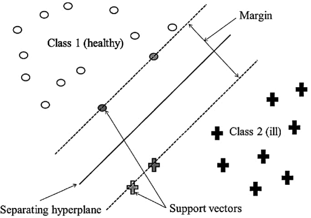
Support vector machines discriminate between two (or more) classes by generating a hyperplane (decision boundary or classifier) which optimally separates the classes (Yu et al. Reference Yu, Liu, Valdez, Gwinn and Khoury2010) (Fig. 1). The easiest separation assumes that the two classes are linearly separable, i.e. there exists a plane that correctly classifies all the points in the two classes. Generally, many linear classifiers are able to separate data into classes. However, only one hyperplane achieves maximum separation. This means that the hyperplane is chosen so that the distance (margin) from the hyperplane to the nearest data point is maximized (Widodo & Yang Reference Widodo and Yang2007) (Fig. 1). The nearest data points used to define the margin are called support vectors, represented by the grey circles and crosses in Fig. 1. The boundary is entirely defined by these support vectors.
The margin, separating hyperplane (decision boundary) and support vectors for a two-class classification problem.

In most cases, linear separation between healthy and ill cases of the input data is a restrictive hypothesis of practical use. Non-linearly separable data is mapped into a high-dimensional space in which the transformed data is linearly separable and thus divided by a hyperplane (Olson & Delen Reference Olson and Delen2008). Mapping into a high-dimensional space can give rise to computational difficulties due to the fact that the dimensionality of the input variable space explodes exponentially (Bennett & Campbell Reference Bennett and Campbell2000). Support vector machines avoid this issue through the use of kernel functions. Kernel functions (usually including linear, polynomial, sigmoid and radial basis functions (RBF)) reduce the complexity of dimensionality by avoiding the step of explicitly mapping the data to a high-dimensional space. This means that the space to be mapped does not have to be known explicitly. The knowledge of the kernel function used is sufficient for all calculations (Schölkopf & Smola Reference Schölkopf and Smola2001). The key parameters, the penalty parameter C and the kernel parameters (altogether hyperparameters), need to be pre-selected to generate an optimal SVM model (Yu et al. Reference Yu, Liu, Valdez, Gwinn and Khoury2010). The parameter C controls over-fitting of the model by specifying the tolerance for misclassification. The kernel parameters control the degree of non-linearity of the model (Olson & Delen Reference Olson and Delen2008). Different kernel functions have differing numbers of kernel parameters. The RBF kernel, for example, has one kernel parameter (gamma) whereas the polynomial kernel has two parameters (gamma and epsilon). Since it is not known which C and kernel parameters are best for one problem, some parameter selection has to be carried out (Olson & Delen Reference Olson and Delen2008). A common way is to apply v-fold cross-validation (v=number of subsets of the training data). Another recommendation is a ‘grid-search’ using cross-validation. In contrast to cross-validation, grid-search does not divide the training dataset into v subsets of equal size followed by testing the classifier of one subset on the remaining v−1 subsets; instead, various pairs of the C and kernel parameters are tried and the one with the best cross-validation accuracy is chosen. For unbalanced data sets, such as in the current case (more healthy observations than diseased observations), accuracy may not be a good criterion for evaluating a model. The receiver operating characteristic (ROC) curve and the related metric area under the curve (AUC) can be more meaningful performance measures since they allow a difference between errors on positive (ill) or negative (healthy) examples (Huang & Ling Reference Huang and Ling2005). Thus, the best pairs of the C (best C) and kernel parameters (e.g. best gamma) were selected using the pair which achieved the best average AUC value. The grid search procedure reduces computational costs and it works well for data, such as in the current study, which do not have many input variables (Olson & Delen Reference Olson and Delen2008).
Procedure of SVMs in disease detection
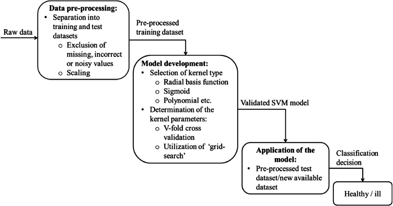
The general procedure for disease detection provided with SVMs is shown in Fig. 2. The raw data for mastitis has to be randomly divided into training and test datasets. After pre-processing of both datasets, including the exclusion of missing values and scaling, the training dataset is used for the model development. The first step is the selection of the kernel function (e.g. linear, polynomial or RBF). For mastitis detection, the RBF as the kernel function performed best and was therefore chosen for both analyses.
A process description of an SVM for disease detection.
After selection of the kernel type, the parameter C and the kernel parameter gamma (best C and best gamma) have to be determined. In the current study, grid search with 5-fold cross-validation was applied, which is recommended by several studies (Ben-Hur et al. Reference Ben-Hur, Ong, Sonnenburg, Schölkopf and Rätsch2008; Olson & Delen Reference Olson and Delen2008; Chang & Lin Reference Chang and Lin2011) in the case of data without many variables.
The validated SVM model can then be used to predict the health status of each cow in the test dataset.
Test procedure
System performance was assessed by comparing these predictions provided by the SVMs with the actual occurrence of diseases.
The day of observation was classified as true positive (TP) if the predicted health status corresponded to an actual case of mastitis, while an undetected day of disease was classified as false negative (FN). Each day in a healthy period was considered as a true negative (TN) case if no alerts were generated and a FP case if an alert was given. The performance of these procedures was evaluated by the parameter sensitivity, block sensitivity, specificity, error rate and accuracy. Sensitivity represented the proportion of correctly detected days of disease of all days of disease as follows:
 $${\rm Sensitivity} = \displaystyle{{{\rm true}\;{\rm positive}} \over {{\rm true}\;{\rm positive} + {\rm false}\;{\rm negative}}}$$
For disease detection, it was not important for all days of a disease block to be recognized, but it was crucial for mastitis to be detected at all, and to be detected early. Therefore, block sensitivity was deemed considerably more important than sensitivity. For the block sensitivity, each disease block was considered a TP case if one or more alerts were given within the defined disease block and a FN case otherwise (Cavero et al. Reference Cavero, Tölle, Rave, Buxadé and Krieter2007; Kramer et al. Reference Kramer, Cavero, Stamer and Krieter2009).
Specificity indicated the proportion of correctly found days of health from all the days of health as follows:
 $${\rm Specificity} = \displaystyle{{{\rm true}\;{\rm negative}} \over {{\rm true}\;{\rm negative} + {\rm false}\;{\rm positive}}}$$
Error rate represented the proportion of days outside the disease periods from all the days on which an alarm was produced as follows:
 $${\rm Error}\;{\rm rate} = \displaystyle{{{\rm false}\;{\rm positive}} \over {{\rm false}\;{\rm positive} + {\rm true}\;{\rm positive}}}$$
Accuracy measured how correctly the SVM identified a given health status. It indicated the proportion of correctly classified days of health and days of disease from all of the classification results as follows:
 $${\rm Accuracy} = \displaystyle{{{\rm true}\;{\rm negative} + {\rm true}\;{\rm positive}} \over \matrix{{\rm true}\;{\rm negative} + {\rm true}\;{\rm positive} \hfill \cr + {\rm false}\;{\rm negative} + {\rm false}\;{\rm positive} \hfill}} $$
The number of TP and FP cows per day was also given; these signified the average number of rightly and wrongly diseased-registered cows per day, respectively. This was an important detail which indicated the effort of the mastitis monitoring system.
RESULTS
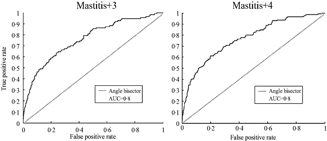
The ROC curves of the training datasets providing the best AUC values for (mastitis definitions) Mastitis+3 and Mastitis+4 are shown in Fig. 3. Both ROC curves exhibit a slope moving away from the angle bisector. In general, the more distant the ROC curve is from the angle bisector, the greater the ability of the monitoring system to differentiate between healthy and ill animals. The closer the AUC value moves to 0·5 (value of the angle bisector) the poorer the test performs. The ROC curves of Mastitis+3 and Mastitis+4 presented below did not vary much from each other, leading to the best AUC value of 0·8 for both definitions.
Receiver operator characteristic (ROC) and their corresponding AUC values for the training process depending on mastitis definition.
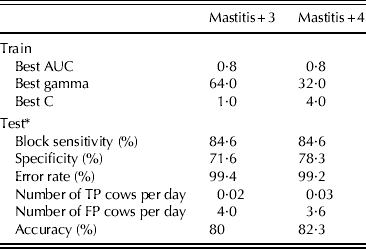
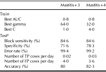
These AUC values were determined by different best pairs of the parameter C and gamma kernel parameter depending on the mastitis definitions (Table 3). For Mastitis+3 the best value of C was 64 whereas the best value of gamma was 1. For Mastitis+4, the best value for the cost parameter C was 32. Gamma was calculated to be 4.
Results of mastitis detection for the training and test datasets depending on the two disease definitions
* Average herd size: 17 cows per day.
The results of the test dataset of each definition are also shown at Table 3. For Mastitis+3, block sensitivity achieved a value of 84·6%, whereas specificity is 71·6%. The error rate, however, was 99·4%. The number of FP cows per day was 4. For the test dataset, the average herd size per day was 17 cows. Therefore, 24% of the animals per day were wrongly classified as ill. Additionally, the accuracy was also provided by the system. For Mastitis+3, the calculated accuracy was 80%.
For the second mastitis definition (Mastitis+4), block sensitivity achieved the same value of 84·6% as the first definition. Showing a value of 78·3%, specificity of Mastitis+4, however, was higher compared to Mastitis+3. The error rate was 99·2%. The number of FP cows per day was also slightly lower than Mastitis+3 (3·6 FP cows per day to 4 FP cows per day). Taking the average herd size into account, 21% of the daily herd would have been mistakenly designated as ill. According to the accuracy of 82·3%, Mastitis+4 performed also slightly better than Mastitis+3.
DISCUSSION
The ROC curves and the AUC values (0·8) show that SVMs were able to distinguish between mastitic and healthy animals, on consideration of the training dataset.
According to Kramer et al. (Reference Kramer, Cavero, Stamer and Krieter2009), monitoring systems in high-throughput milking parlours, such as in Karkendamm, should reach a block sensitivity of at least 70%. The results indicate that the block sensitivities (84·6%) are above this minimum system requirement for both mastitis definitions. Thus, the detection performance of the monitoring system of both disease definitions can be deemed acceptable. Specificities, however, are only c. 80% or lower. Additionally, the error rates are too high at c. 99%. The error rate is mainly affected by the number of FP alerts, which was also high in the present study, showing >0·2 of the herd per day falsely classified as diseased. This results in more workload for the farmer accompanied by a loss of confidence in the monitoring system. Such unfavourable results can be caused by several factors.
First, the disease definition is very important and subsequently influences the classification results. In the current study, an animal was considered to be ill if a treatment occurred. These treatments were carried out by a qualified veterinarian and can therefore be considered reliable.
According to Hogeveen et al. (Reference Hogeveen, Kamphuis, Steeneveld and Mollenhorst2010), an alert should be given before clinical signs are visible so that a treatment has a greater efficiency and reflects the implementations of practice. Therefore, disease blocks were analysed before treatment occurred. Bareille et al. (Reference Bareille, Beaudeau, Billon, Robert and Faverdin2003) stated that mastitis affects milk production parameters at 3–4 days before visual onset of this disease. Thus, 3- and 4-day periods before clinical signs were chosen for mastitis detection.
However, the choice of the length of the disease blocks has varied widely (1–17 days) in past research on disease detection (de Mol et al. Reference De Mol, Kroeze, Achten, Maatje and Rossing1997; Hogeveen et al. Reference Hogeveen, Kamphuis, Steeneveld and Mollenhorst2010). For instance, de Mol & Woldt (Reference De Mol and Woldt2001) indicated a period of 7 days before mastitis treatment occurred. Cavero et al. (Reference Cavero, Tölle, Henze, Buxadé and Krieter2008) utilized disease blocks of 5 days (day of treatment plus 2 days prior and after treatment) for mastitis detection. In general, block sensitivity increases if longer periods are considered. In consequence, a comparison of model performance with other studies is difficult. Other reasons for the results obtained in the current study might be attributed to the indicator variables. Due to their easy availability at reasonable costs, the sensor-measured data of MY and MEC have been used in several studies (Cavero et al. Reference Cavero, Tölle, Henze, Buxadé and Krieter2008; Gonzalez et al. Reference Gonzalez, Tolkamp, Coffey, Ferret and Kyriazakis2008; Hagnestam-Nielsen et al. Reference Hagnestam-Nielsen, Emanuelson, Berglund and Strandberg2009; Kramer et al. Reference Kramer, Cavero, Stamer and Krieter2009; Lukas et al. Reference Lukas, Reneau, Wallace, Hawkins and Munoz-Zanzi2009). Compared to the current study, Cavero et al. (Reference Cavero, Tölle, Henze, Buxadé and Krieter2008) reached higher block sensitivities (92·9%) and specificities (93·9%) by applying of fuzzy logic. However, the MEC values of Cavero et al. (Reference Cavero, Tölle, Henze, Buxadé and Krieter2008) were measured at the quarter level of each cow, which gives better detection performance (Hogeveen et al. Reference Hogeveen, Kamphuis, Steeneveld and Mollenhorst2010). Additionally, there is a high variation in the recorded traits between cows but also within cows causing a high number of FP cows per day. Cows always react individually to diseases (Kramer et al. Reference Kramer, Cavero, Stamer and Krieter2009; Lukas et al. Reference Lukas, Reneau, Wallace, Hawkins and Munoz-Zanzi2009; Brandt et al. Reference Brandt, Haeussermann and Hartung2010); hence, it is very difficult to detect a unique pattern in cows suffering and/or developing a disease from the indicator variables. Cavero et al. (Reference Cavero, Tölle, Rave, Buxadé and Krieter2007) and Miekley et al. (Reference Miekley, Traulsen and Krieter2012) implemented a detection system based on univariate traits, expecting multivariate monitoring methods to compensate for high variation in each trait und thus improves the results of disease detection systems.
Support vector machines enable such multivariate considerations. Martiskainen et al. (Reference Martiskainen, Järvinen, Skön, Tiirikainen, Kolehmainen and Mononen2009) and Hokkanen et al. (Reference Hokkanen, Hänninen, Tiusanen and Pastell2011) used SVMs to classify cow and calf behaviour, respectively, based on accelerometer data. Both studies stated their potential for pattern recognition and classification. Martiskainen et al. (Reference Martiskainen, Järvinen, Skön, Tiirikainen, Kolehmainen and Mononen2009) found an overall sensitivity of the utilized patterns (standing, lying, lame walking) of 78%. According to our knowledge, SVMs have so far not been applied to mastitis detection in dairy cows.
Although the results (which need further improvement) might not seem promising, there are some appealing features of SVMs for disease detection. First of all, SVMs are easy to implement, are able to adapt flexibly to different kinds of classification problems and the final results are stable and reproducible (Bennett & Campbell Reference Bennett and Campbell2000). A great advantage of SVMs is the ability to handle unbalanced datasets, which is applicable for many datasets in bioinformatics, especially in disease detection as in the current study. Additionally, analyses of more than two different classes, such as in Martiskainen et al. (Reference Martiskainen, Järvinen, Skön, Tiirikainen, Kolehmainen and Mononen2009), are possible. Thus, considerations of each mastitis are feasible instead of the division into healthy or mastitis. This might improve the results. However, such approaches necessitate the extension of the training dataset incorporating enough observations of each category or disease. Unfortunately, the main limitation of SVMs is a vast increase in computer and storage time with the number of training examples (Bottou et al. Reference Bottou, Chapelle, DeCoste and Weston2007; Ben-Hur et al. Reference Ben-Hur, Ong, Sonnenburg, Schölkopf and Rätsch2008). Therefore, the dataset of the current study contained data from cows only in 2010–2011, although more data from previous years were available. Recently, new methods to overcome this problem, called reduced support vector machines (RSVM), have been introduced (Bottou et al. Reference Bottou, Chapelle, DeCoste and Weston2007). However, there are some concerns about the test accuracy of the RSVM and further research has to be carried out.
Sensitivity, specificity and error rate are well known quality parameters characterising the performance of a detection system. The sensitivity and specificity of a test, however, are independent of the occurrence of the event (mastitis) to be detected (Hogeveen et al. Reference Hogeveen, Kamphuis, Steeneveld and Mollenhorst2010) giving equal weight to each class (healthy, ill). Nevertheless, the classes are highly imbalanced.
CONCLUSION
Support vector machines provide an opportunity for the early detection of mastitis. This classification method has appealing features for its implementation and usage for biological data (e.g. handling of unbalanced data). Although block sensitivities above 70% were achieved, error rates and number of FP cows per day were too high. Given the settings of this study (i.e. indicator variables), SVMs do not seem to be directly implementable into monitoring systems in practice.