1 Introduction
The Rayleigh–Bénard cell, which consists of a fluid layer heated from below and cooled from above, is a useful model system to investigate turbulent thermal convection. It is very widely used, for both experimental and numerical studies (Ahlers, Grossmann & Lohse Reference Ahlers, Grossmann and Lohse2009; Chillà & Schumacher Reference Chillà and Schumacher2012). The main non-dimensional control parameter is the Rayleigh number,  $Ra$,
 $$\begin{eqnarray}Ra=\frac{g\unicode[STIX]{x1D6FC}\unicode[STIX]{x0394}Th^{3}}{\unicode[STIX]{x1D708}\unicode[STIX]{x1D705}},\end{eqnarray}$$
which compares the buoyancy forcing and the diffusive terms, where  $g$ is the acceleration due to gravity,
 $\unicode[STIX]{x1D6FC}$ the thermal expansion coefficient,
 $\unicode[STIX]{x0394}T$ the temperature difference,
 $h$ the cell height,
 $\unicode[STIX]{x1D708}$ the kinetic viscosity and
 $\unicode[STIX]{x1D705}$ the thermal diffusivity. Turbulent thermal convection is obtained when
 $Ra>10^{7}$. The other control parameters are the Prandtl number,
 $Pr$, and the cell aspect ratios,
 $\unicode[STIX]{x1D6E4}_{xz}$ and
 $\unicode[STIX]{x1D6E4}_{yz}$,
 $$\begin{eqnarray}Pr=\frac{\unicode[STIX]{x1D708}}{\unicode[STIX]{x1D705}}\quad \text{and}\quad \unicode[STIX]{x1D6E4}_{xz}=\ell /h\quad \text{and}\quad \unicode[STIX]{x1D6E4}_{yz}=D/h,\end{eqnarray}$$
where  $\ell$ is the cell width and
 $D$ the cell depth.
The flow can be characterized by global quantities, such as the global heat transfer efficiency, which can be quantified by the Nusselt number,  $Nu$,
 $$\begin{eqnarray}Nu=\frac{\dot{q}h}{\unicode[STIX]{x1D706}\unicode[STIX]{x0394}T},\end{eqnarray}$$
where  $\dot{q}$ is the thermal flux, and
 $\unicode[STIX]{x1D706}$ is the thermal conductivity. When heat is transported by convection, the Nusselt number is larger than unity. There have been a lot of efforts to find the relation between the Nusselt number and the control parameters (Castaing et al. Reference Castaing, Gunaratne, Heslot, Kadanoff, Libchaber, Thomae, Wu, Zaleski and Zanetti1989; Shraiman & Siggia Reference Shraiman and Siggia1990; Grossmann & Lohse Reference Grossmann and Lohse2000, Reference Grossmann and Lohse2011), in particular in the high Rayleigh number limit where the flow is highly turbulent (see Ahlers et al. (Reference Ahlers, Grossmann and Lohse2009) and Chillà & Schumacher (Reference Chillà and Schumacher2012) for reviews of experiments, numerical simulations and scaling theories).
Another approach is to investigate quantities, such as velocity and temperature. Experimental investigation of the velocity field often requires optical access to the cell, and the seeding of particles, (Qiu & Tong Reference Qiu and Tong2001; Xia, Sun & Zhou Reference Xia, Sun and Zhou2003; Zhou et al. Reference Zhou, Li, Lu and Liu2011; Ni, Huang & Xia Reference Ni, Huang and Xia2012; Liot et al. Reference Liot, Gay, Salort, Bourgoin and Chillà2016a, Reference Liot, Ehlinger, Rusaouën, Coudarchet, Salort and Chillà2017). However, optical access is not always possible, in particular in the cryogenic set-ups (Chavanne et al. Reference Chavanne, Chillà, Castaing, Hébral, Chabaud and Chaussy1997; Niemela et al. Reference Niemela, Skrbek, Sreenivasan and Donnelly2000; Urban et al. Reference Urban, Hanzelka, Musilová, Králik, Mantia, Srnka and Skrbek2014), or in the Göttingen sulphur hexafluoride experiment (He et al. Reference He, Funfschilling, Bodenschatz and Ahlers2012a), and most traditional local velocity sensors – hot-wires, Pitot tubes – cannot operate in the velocity range of thermal convection. The alternative method which has been used to infer velocity estimates in these systems is based on the correlation of two or more thermometers (Wu Reference Wu1991; Chavanne et al. Reference Chavanne, Chillà, Chabaud, Castaing and Hébral2001; Sun & Xia Reference Sun and Xia2005; He et al. Reference He, van Gils, Bodenschatz and Ahlers2015; Musilová et al. Reference Musilová, Králik, Mantia, Macek, Urban and Skrbek2017).
The experimental investigation of the temperature field is a difficult matter, because of the low amplitude of temperature fluctuations in the bulk. Direct measurements can be achieved with thermochromic liquid crystals (Du & Tong Reference Du and Tong2001; Stasiek & Kowalewski Reference Stasiek and Kowalewski2002; Zhou, Sun & Xia Reference Zhou, Sun and Xia2007a; Zhou & Xia Reference Zhou and Xia2010; Tummers & Steunebrink Reference Tummers and Steunebrink2019), or temperature sensitive fluorescent dye (Sakakibara & Adrian Reference Sakakibara and Adrian2004). Although quite successful, the drawbacks of these methods are the technical difficulty in increasing the sensitivity and the response time, enough for the very large Rayleigh number limit. The simple alternative is the imaging of the optical index gradient using either shadowgraph (Jenkins Reference Jenkins1988; de Bruyn et al. Reference de Bruyn, Bodenschatz, Morris, Trainoff, Hu, Cannel and Ahlers1996; Trainoff & Cannell Reference Trainoff and Cannell2002; Xi, Lam & Xia Reference Xi, Lam and Xia2004; Hattori et al. Reference Hattori, Bartos, Norris, Kirkpatrick and Armfield2013; Wang et al. Reference Wang, Lai, Song and Tong2018), or schlieren (Ciliberto, Francini & Simonelli Reference Ciliberto, Francini and Simonelli1985; Chillà et al. Reference Chillà, Ciliberto, Innocenti and Pampaloni1993; Dalziel, Hugues & Sutherland Reference Dalziel, Hugues and Sutherland2000; Salort et al. Reference Salort, Liot, Rusaouen, Seychelles, Tisserand, Creyssels, Castaing and Chillà2014; Raffel Reference Raffel2015; Taberlet et al. Reference Taberlet, Plihon, Auzémery, Sautel, Panel and Gibaud2018). The advantage is that these methods are straightforward to implement, non-invasive and are fairly sensitive. However, the flow pattern is averaged over the depth of the cell.
It can be mentioned also that there have been studies which infer plume statistics from one local temperature sensor. For example, Gauthier et al. (Reference Gauthier, Salort, Bourgeois, Garden, du Puits, Thess and Roche2009) evidenced a transition in the temperature fluctuation statistics in the ultimate regime of convection, Zhou et al. (Reference Zhou, Xie, Sun and Xia2016) studied the width and amplitude statistics of plumes with Rayleigh numbers ranging from 2 × 10⁸ to 1. 85 × 1010. There are also many investigations of temperature profiles (Tilgner, Belmonte & Libchaber Reference Tilgner, Belmonte and Libchaber1993; du Puits et al. Reference du Puits, Resagk, Tilgner, Busse and Thess2007; Ahlers et al. Reference Ahlers, Bodenschatz, Funfschilling, Grossmann, He, Lohse, Stevens and Verzicco2012; Wei & Ahlers Reference Wei and Ahlers2014; Xie et al. Reference Xie, Cheng, Hu and Xia2019).
The first goal of this paper is to discuss some quantitative information that can be inferred from an experimental shadowgraph image in the Rayleigh–Bénard system. The recent study of Wang et al. (Reference Wang, Lai, Song and Tong2018) showed that adequate post-processing effectively allows us to derive useful quantities (in their case, statistical properties of eruption events of thermal plumes in a vertical thin disk convection experiment). To that end, experimental shadowgraph images are compared with direct numerical simulations (DNS) of a Rayleigh–Bénard cell, from which a synthetic shadowgraph image can be computed from the temperature field, under the assumption that geometrical optics holds (Trainoff & Cannell Reference Trainoff and Cannell2002). The results are compared against the fluid velocity fields in the case of the computer simulations, and against particle image velocimetry (PIV) measurements in similar conditions in the case of the experimental data.
One important open question in turbulent thermal convection is to understand and accurately model the flow and heat transfer efficiency in the highly turbulent limit. Kraichnan (Reference Kraichnan1962) predicted that turbulent boundary layers would increase the scaling law for the Nusselt number to the asymptotic regime
 $$\begin{eqnarray}Nu\sim Ra^{1/2}[\log Ra]^{-3/2}.\end{eqnarray}$$
The search for this asymptotic regime, and for evidence of turbulent boundary layers in turbulent Rayleigh–Bénard convection, has been a long-term effort for many groups and is still a very active topic (Chavanne et al. Reference Chavanne, Chillà, Castaing, Hébral, Chabaud and Chaussy1997; Niemela et al. Reference Niemela, Skrbek, Sreenivasan and Donnelly2000; Chillà et al. Reference Chillà, Rastello, Chaumat and Castaing2004; Funfschilling, Bodenschatz & Ahlers Reference Funfschilling, Bodenschatz and Ahlers2009; Roche et al. Reference Roche, Gauthier, Kaiser and Salort2010; Grossmann & Lohse Reference Grossmann and Lohse2011; He et al. Reference He, Funfschilling, Nobach, Bodenschatz and Ahlers2012b; Ahlers, Bodenschatz & He Reference Ahlers, Bodenschatz and He2017; Zhu et al. Reference Zhu, Mathai, Stevens, Verzicco and Lohse2018a; Bouillaut et al. Reference Bouillaut, Lepot, Aumaître and Gallet2019; Urban et al. Reference Urban, Hanzelka, Králik, Macek and Musilová2019). However, the range of Rayleigh numbers that must be achieved to enter this regime is very high, and not easily accessible to experiments or numerical simulations. Experiments are possible only with non-conventional fluids such as cryogenic helium and pressurized sulphur hexafluoride. Additionally, the threshold seems to highly depend on small details, which led to apparent contradictions between experimental results.
An alternative approach is to attempt to lower the threshold Reynolds number with a surface roughness, and seek evidence of a transition to turbulent boundary layers at a lower and more accessible Rayleigh number. While this approach has proved at least partially successful in the sense that roughness surfaces do trigger enhanced heat transfer, and a higher scaling exponent (Salort et al. Reference Salort, Liot, Rusaouen, Seychelles, Tisserand, Creyssels, Castaing and Chillà2014; Liot et al. Reference Liot, Salort, Kaiser, du Puits and Chillà2016b; Toppaladoddi, Succi & Wettlaufer Reference Toppaladoddi, Succi and Wettlaufer2017; Xie & Xia Reference Xie and Xia2017; Zhu et al. Reference Zhu, Stevens, Verzicco and Lohse2017, Reference Zhu, Verschoof, Bakhuis, Huisman, Verzicco, Sun and Lohse2018b), the detailed mechanisms are still open for debate, and the dynamics is very rich. In particular, Zhu et al. (Reference Zhu, Stevens, Verzicco and Lohse2017) and MacDonald et al. (Reference MacDonald, Hutchins, Lohse and Chung2019) claim that the roughness-facilitated local 1/2 scaling is different in nature from the high Rayleigh number asymptotically 1/2 scaling (ultimate regime). In contrast, Toppaladoddi et al. (Reference Toppaladoddi, Succi and Wettlaufer2017) claim that roughness facilitates the attainment of the ultimate regime. The present paper will not settle this debate, but will contribute new experimental and numerical data to the discussion. Thermal convection over rough surfaces is also an important question for real natural and industrial applications, since most natural surfaces are not hydrodynamically smooth. This is why the analysis of the heat transfer efficiency in thermal convection over rough surfaces has triggered both experimental (Du & Tong Reference Du and Tong1998; Ciliberto & Laroche Reference Ciliberto and Laroche1999; García et al. Reference García, Solano, Vicente and Viedma2012; Wei et al. Reference Wei, Chan, Ni, Zhao and Xia2014; Xie & Xia Reference Xie and Xia2017; Rusaouen et al. Reference Rusaouen, Liot, Salort, Castaing and Chillà2018; Tummers & Steunebrink Reference Tummers and Steunebrink2019), theoretical (Shishkina & Wagner Reference Shishkina and Wagner2011; Goluskin & Doering Reference Goluskin and Doering2016), and numerical efforts (Wagner & Shishkina Reference Wagner and Shishkina2015; Toppaladoddi et al. Reference Toppaladoddi, Succi and Wettlaufer2017; Zhu et al. Reference Zhu, Stevens, Verzicco and Lohse2017; Zhang et al. Reference Zhang, Sun, Bao and Zhou2018; Zhu et al. Reference Zhu, Stevens, Shishkina, Verzicco and Lohse2019).
The most consensual result is that a heat transfer enhancement is triggered when the thermal boundary layer thickness matches the height of the roughness size. The nature of the enhanced regime may, however, differ; some observe an increase of the scaling exponent (Roche et al. Reference Roche, Castaing, Chabaud and Hébral2001; Qiu, Xia & Tong Reference Qiu, Xia and Tong2005; Tisserand et al. Reference Tisserand, Creyssels, Gasteuil, Pabiou, Gibert, Castaing and Chillà2011), and some observe only an increase of the prefactor (Du & Tong Reference Du and Tong1998). There is also a competition between an enhancement of plume emission by the rough surface, as directly evidenced by Du & Tong (Reference Du and Tong2000) with thermochromic liquid crystals, and an enhancement due to higher turbulence intensity (Salort et al. Reference Salort, Liot, Rusaouen, Seychelles, Tisserand, Creyssels, Castaing and Chillà2014).
Recent works suggest that three regimes can be identified (Xie & Xia Reference Xie and Xia2017; Zhu et al. Reference Zhu, Stevens, Verzicco and Lohse2017; Rusaouen et al. Reference Rusaouen, Liot, Salort, Castaing and Chillà2018; Belkadi Reference Belkadi2019; Tummers & Steunebrink Reference Tummers and Steunebrink2019): Regime I when the surface is hydrodynamically smooth, Regime II when the plate becomes hydrodynamically rough and triggers a change in the scaling law exponent and Regime III when the heat transfer enhancement saturates due to the viscous boundary layer cross-over. These regimes allow us to understand the apparent discrepancies previously reported.
In this work, the experiment and the numerical simulation are not in the same regime. The experiment is operated in Regime II, and the numerical simulation in Regime III. Indeed, we use the numerical simulation, where all the fields are known, to study the processing tools. The results can be compared to experimental measurements, because the processing tools are the same to study all regimes. The limit of the plume detection method does not depend on the regime, and comparison remains relevant.
Therefore, we present the experiment and the numerical simulation side by side, even though the statistical features of the plumes in both cases are not expected to be similar. Once the detection method is established, the fact that the experiment and the numerics lie respectively in Regime II and Regime III, allows us to highlight particular features of each regime.
The second goal of this paper is thus to use the quantitative information on the thermal plumes, provided by the analysis of the shadowgraph image, to compare the statistics of the warm plumes emitted by the rough surface, with those of the cold plumes emitted by the smooth surface, in both cases. We previously showed that the smooth half-cell behaves, at first order, as a smooth convection cell, at least in the range of Rayleigh numbers that we investigate, where roughness triggers more intense turbulence fluctuations. And the rough half-cell essentially behaves as a rough convection cell. These allow us to directly compare the dynamics of smooth and rough plates, within the same system.
The paper is structured with the experimental and numerical results side by side. The experimental and numerical configurations are described in § 2. The methods to obtain experimental and numerical shadowgraph images are described in § 3. The statistics of plume velocity and plume density, based on the analysis of spatio-temporal diagrams, is discussed in § 4.
2 Rayleigh–Bénard convection cells
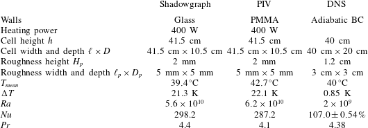
Experimental and numerical configurations of the Rayleigh–Bénard cells. BC: boundary conditions; PMMA: PolyMethyl MethAcrylate. The DNS Nusselt number is given as the mean and its deviation of several estimations as proposed by Shishkina et al. (Reference Shishkina, Stevens, Grossmann and Lohse2010).

2.1 Experimental configuration
The experimental convection cell is a 41. 5 cm × 10. 5 cm × 41. 5 cm rectangular cell, with aspect ratios  $\unicode[STIX]{x1D6E4}_{xz}=1$ and
 $\unicode[STIX]{x1D6E4}_{yz}=0.253$. The details of this cell have been published in our previous works (Salort et al. Reference Salort, Liot, Rusaouen, Seychelles, Tisserand, Creyssels, Castaing and Chillà2014; Liot et al. Reference Liot, Ehlinger, Rusaouën, Coudarchet, Salort and Chillà2017). The only difference is that the walls are now made of glass, instead of PMMA, to avoid spurious optical index gradients in the walls. Because the heat conductivity of glass is larger than PMMA, this means that we have to work with a bulk temperature close to the temperature of the room, to avoid heat flux across the walls. Because the cell cannot be fully insulated to preserve optical access, only a sufficiently high heating power can be used for the heat losses to remain negligible. The experimental conditions are summarized in table 1.
We recall the main characteristics. The bottom plate is rough, made of aluminium alloy (5083) anodized in black. The roughness consists in periodic parallelepiped roughness elements  $2~\text{mm}\times 5~\text{mm}$, machined directly into the plate. The top plate is a 4 cm thick smooth copper plate coated with a thin layer of nickel. Plate temperatures are measured with PT-100 temperature sensors. The bottom plate is heated with Kapton heaters glued at the bottom of the plate, and powered with a constant voltage. The top plate is cooled with the circulation of a mixture of water and ethylene glycol, flowing into a tight meander machined at the top of the copper plate, and temperature regulated by a Lauda RP845 chiller.
2.2 Numerical configuration
The numerical configuration is detailed in Belkadi (Reference Belkadi2019). We consider a physical configuration close to the experimental one: a 40 cm high Rayleigh–Bénard cell of square vertical cross-section, filled with water at the mean temperature ( $T_{mean}$), with a rough bottom plate and a smooth top plate. The roughness consists in regularly spaced parallelepiped roughness elements. The main characteristics of the physical problem are given in table 1. In this paper, the Rayleigh number is set to
 $Ra=2\times 10^{9}$.
The fluid flow is governed by the Boussinesq equations, where the gravity vector  $\boldsymbol{g}$ is aligned with the
 $-\boldsymbol{e}_{z}$ direction. A no-slip condition for the velocity field is applied on the walls. The temperature difference
 $\unicode[STIX]{x0394}T$ is imposed on the top and bottom walls including the roughness element surfaces by applying isothermal boundary conditions (
 $T_{top}=T_{mean}-\unicode[STIX]{x0394}T/2$ and
 $T_{bot}=T_{mean}+\unicode[STIX]{x0394}T/2$), while adiabaticity
 $\unicode[STIX]{x2202}T/\unicode[STIX]{x2202}\boldsymbol{n}=0$ is satisfied on sidewalls.
The Boussinesq solver, called SUNFLUIDH, uses a finite volume discretization on staggered grids. The time marching is treated by a semi-implicit scheme combined with a prediction–correction scheme for the velocity–pressure coupling, with a global second-order accuracy. The pressure problem is solved by a multi-grid method. Roughness elements are modelled through a loop truncation technique. A domain decomposition method using MPI is implemented for parallel computation.
The simulation has been performed on a non-uniform grid with 768 × 384 × 768 cells in the ( $\boldsymbol{e}_{x},\boldsymbol{e}_{y},\boldsymbol{e}_{z}$) directions respectively. The mesh has been particularly refined between roughness elements, and the cell size is everywhere finer than the Kolmogorov scale. The time step, equal to 0.011925 s, meets the Courant–Friedrichs–Lewy criterion. The spatial resolution has been checked by evaluating the numerical convergence of time-averaged Nusselt numbers obtained by different methods (space averages on the horizontal planes or volume averages based on the dissipation rates) as proposed by Shishkina et al. (Reference Shishkina, Stevens, Grossmann and Lohse2010). Statistics have been determined over more than one hour and 20 min (physical time) to obtain these values. They converge with a deviation of less than 1 % of the average Nusselt number, as specified in table 1.
3 Shadowgraph images
3.1 Experimental set-up
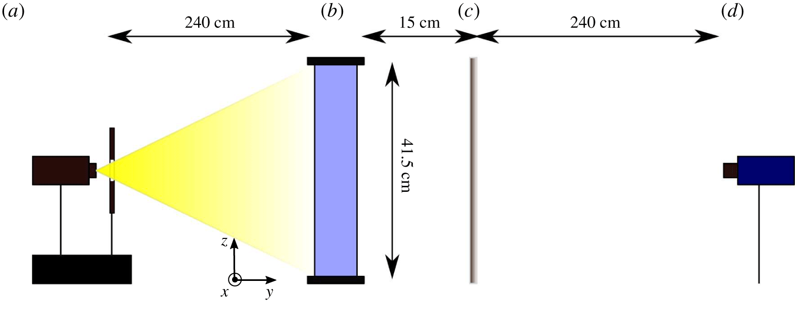
There are several possible shadowgraph set-ups (Settles Reference Settles2001). The classical, and most used set-up requires parallel incident light. This is obtained with either a concave mirror or a lens. However, for fields of view larger than 15 cm, this is impractical, or would require the use of a parabolic telescope mirror. The alternative, that we used in this work, is to implement direct shadowgraphy in diverging light with a small, or punctual, bright source of light. This is the method originally used by Marat (Reference Marat1780).
Optical set-up for the shadowgraph experiment. (a) Quartz iodine lamp, heat absorbing filter and diaphragm; (b) Rayleigh–Bénard convection cell; (c) ground glass diffuser; (d) PCO 1600 camera.

In this work, the convection cell is illuminated by a punctual source of white light, as shown in figure 1. The cell depth is four times smaller than the width and height, so that the flow is quasi-bidimensional and the integration along the depth does not significantly blur the convection patterns.
The shadowgraph pattern is captured on a projection screen, and recorded with a PCO 1600 digital camera. The resolution is  $1600~\text{pixels}\times 1200~\text{pixels}$ and the frame rate is 10 f.p.s., corresponding to 800 images per turnover, where the turnover time
 $T_{turnover}$ is
 $$\begin{eqnarray}T_{turnover}=\frac{4h}{v_{wind}},\end{eqnarray}$$
and  $v_{wind}\approx 2~\text{cm}~\text{s}^{-1}$. Twenty series of 2400 images were recorded, amounting to 80 min, which is 60 turnover times. The recorded image,
 $I(x,z)$, is determined by the second derivative of the refractive index,
 $$\begin{eqnarray}\frac{I(x,z)}{I_{0}}=\frac{\unicode[STIX]{x1D6FE}(\unicode[STIX]{x1D702}-\unicode[STIX]{x1D6FE})}{\unicode[STIX]{x1D702}}\int _{0}^{D}\left(\frac{\unicode[STIX]{x2202}^{2}}{\unicode[STIX]{x2202}x^{2}}+\frac{\unicode[STIX]{x2202}^{2}}{\unicode[STIX]{x2202}z^{2}}\right)(\ln n)\,\text{d}y,\end{eqnarray}$$
where  $I_{0}$ is the intensity of the incident light,
 $\unicode[STIX]{x1D6FE}=15~\text{cm}$ is the distance between the cell and the projection screen and
 $\unicode[STIX]{x1D702}=265~\text{cm}$ is the distance between the light source and the projection screen. Since in this set-up,
 $\unicode[STIX]{x1D702}/\unicode[STIX]{x1D6FE}\gg 1$, the sensitivity function
 $\unicode[STIX]{x1D6FE}(\unicode[STIX]{x1D702}-\unicode[STIX]{x1D6FE})/\unicode[STIX]{x1D702}$ is not very large, and nearly proportional to
 $\unicode[STIX]{x1D6FE}$, and the magnification factor
 $m$
 $$\begin{eqnarray}m=\frac{\unicode[STIX]{x1D702}}{\unicode[STIX]{x1D702}-\unicode[STIX]{x1D6FE}},\end{eqnarray}$$
is close to unity. This is close to the case of parallel light, and is sufficient to image plumes in Rayleigh–Bénard convection.
In practice, in the case of thermal convection, the variation of optical index is caused by variations of temperature, which are small in the bulk. Equation (3.2) can thus be written in a simpler form,
 $$\begin{eqnarray}\frac{I(x,z)}{I_{0}}\propto \unicode[STIX]{x1D6FE}\int _{0}^{D}\left(\frac{\unicode[STIX]{x2202}^{2}T}{\unicode[STIX]{x2202}x^{2}}+\frac{\unicode[STIX]{x2202}^{2}T}{\unicode[STIX]{x2202}z^{2}}\right)\,\text{d}y.\end{eqnarray}$$
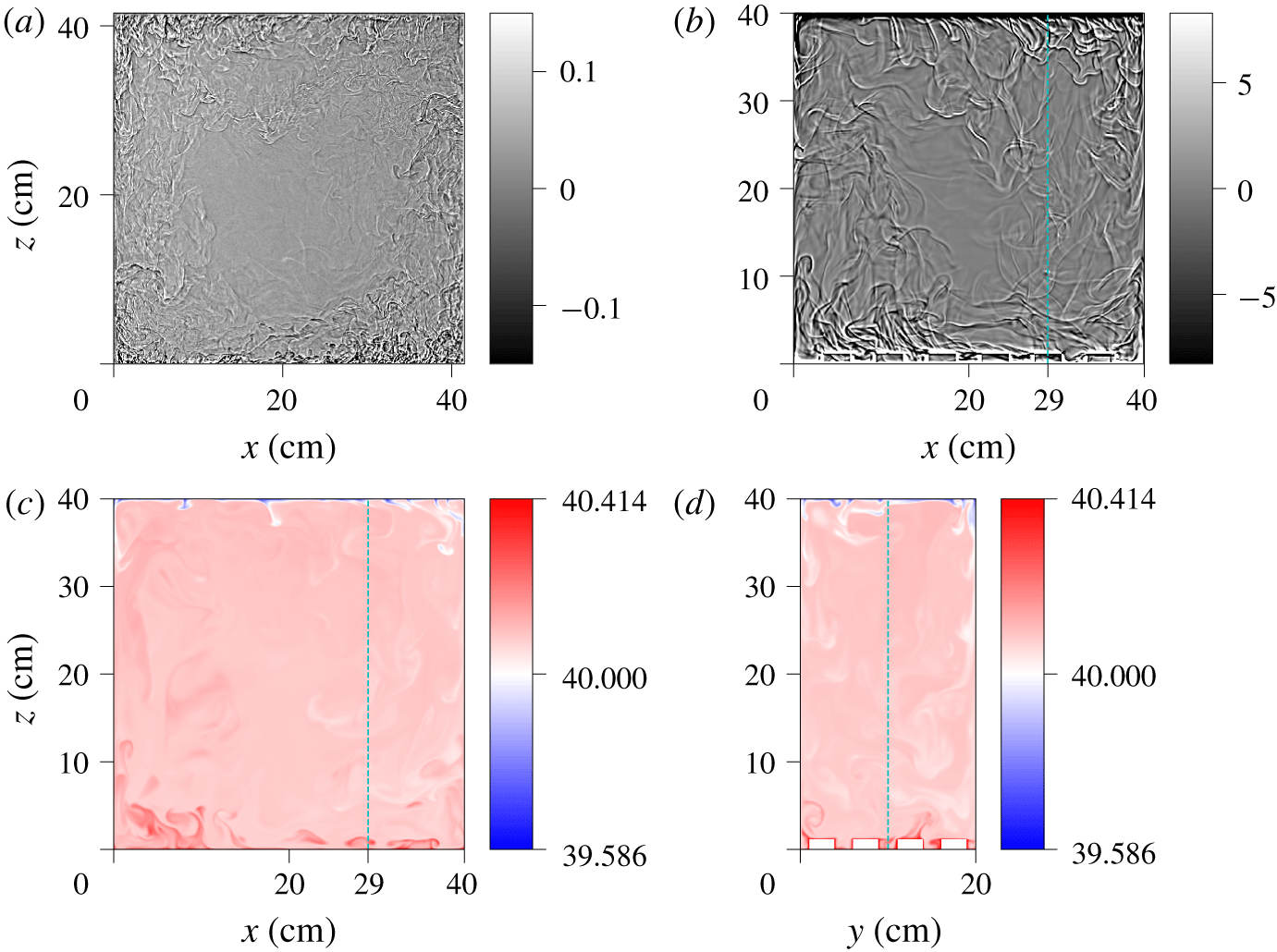
(a) Experimental full field shadowgraph image at  $Ra=5.6\times 10^{10}$. The colour bar indicates the relative light intensity,
 $I(x,z)/I_{0}(x,z)-1.0$, where
 $I_{0}(x,z)$ is the time-averaged image of the cell (see text). (b) Synthetic full field shadowgraph image from the numerical simulation at
 $Ra=2\times 10^{9}$, computed from the full three-dimensional temperature field using (3.4). (c) Snapshot of the mid-plane (
 $y=10~\text{cm}$) temperature of the numerical simulation at the same time as the shadowgraph. Only the fluid trapped between the roughness elements is visible at this particular position (see the dashed line in (d)). (d) Snapshot of the transverse (
 $x=29~\text{cm}$) temperature. The blue dashed lines in (b,c,d) show the intersection of the planes.

A snapshot of the experimental shadowgraph is shown in figure 2(a). The raw image is numerically enhanced by dividing the field by the reference image  $I_{0}(x,z)$. This reference image can be obtained with the fluid at rest, or by averaging the recording in time. Indeed, the plume pattern is lighter and darker, and averages to zero. We found no practical difference between the two estimates of
 $I_{0}(x,z)$, and found it more practical to use the time average. As shown in the figure, the variations of light intensity induced by the thermal plumes is
 $\pm$20 %.
3.2 Synthetic shadowgraph in numerical simulations
A numerical shadowgraph can be derived from the temperature field using (3.4), at regular time steps 0.5366 s, and produces a sequence of synthetic images, similar to those obtained in the experiments (see figure 2b). To that end, 5524 integrated two-dimensional (2-D) Laplacian fields were saved, spanning over 49 min in dimensional time, with a numerical frame rate of 1.86 f.p.s. The mean wind is  $0.4~\text{cm}~\text{s}^{-1}$, so the numerical frame rate corresponds to 745 images per turnover, and a total recording time of 7.4 turnovers. The time resolution is therefore of a similar order of magnitude as the experimental recording frame rate, but with a shorter duration in terms of turnover times. However, the Rayleigh number is also smaller, so fewer turnover times are sufficient to reach statistical convergence. This allows us to use the same type of image, and similar processing tools, both for the experiment and the numerics.
The comparison with the experimental shadowgraph, shown in figure 2(a), evidences more plumes, and smaller plumes in the experiment. This is due to the difference in Rayleigh numbers. The numerical shadowgraph of the present work can also be compared to experimental shadowgraphs obtained in water at lower Rayleigh numbers (Wang et al. Reference Wang, Lai, Song and Tong2018; Tummers & Steunebrink Reference Tummers and Steunebrink2019), and higher Rayleigh numbers (Xie & Xia Reference Xie and Xia2017).
In this paper, we focus on the analysis of the shadowgraph itself, and use the numerical simulations to validate the interpretation of the field. With that aim, it is not necessary to have experiments and numerical simulations in the same range of Rayleigh numbers. The role of the Rayleigh number, and the various regimes in rough cells, is beyond the scope of the present work, but would benefit from the tools described here, in particular in situations where shadowgraphs may be the only available investigation tool.
A snapshot of the mid-plane temperature field is shown in figure 2(c). The mean temperature value is larger than  $40\,^{\circ }\text{C}$, because of the enhanced heat transport of the rough surface at the bottom. Only a few plumes can be identified on the temperature snapshot, both on the top and bottom surfaces, while many more plumes can be seen on the numerical shadowgraph. This is due to the integration along
 $y$ in the latter, which adds up contributions of plumes at several
 $y$ positions, as well as the contribution of their 3-D structure. The far lower number of visible plumes on the mid-plane temperature, versus integrated fields such as the shadowgraph, can also be observed experimentally, e.g. with laser-induced fluorescence (Sakakibara & Adrian Reference Sakakibara and Adrian2004), or thermochromic liquid crystals (Du & Tong Reference Du and Tong2001), but there are few direct comparisons.
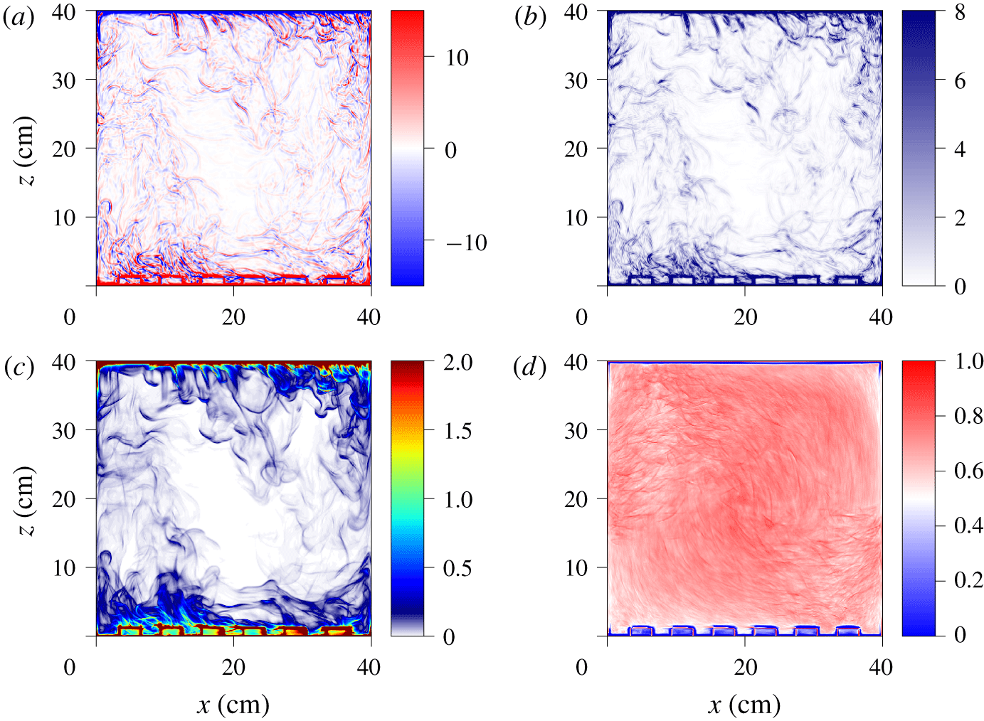
Snapshot of the numerical fields at  $Ra=2\times 10^{9}$. (a) Numerical shadowgraph computed with (3.4). (b) Local variance of the shadowgraph image. (c) Local 2-D thermal dissipation rate, averaged over
 $y$,
 $\langle \unicode[STIX]{x1D716}_{\unicode[STIX]{x1D703},2D}\rangle _{y}=\langle \unicode[STIX]{x1D705}((\unicode[STIX]{x2202}_{x}T)^{2}+(\unicode[STIX]{x2202}_{z}T)^{2})\rangle _{y}$, normalized by the global thermal dissipation rate,
 $\langle \unicode[STIX]{x1D716}_{\unicode[STIX]{x1D703}}\rangle _{x,y,z,t}=\unicode[STIX]{x1D705}(\unicode[STIX]{x0394}T^{2}/h^{2})Nu$. (d) Time-averaged cross-correlation between the local variance of the shadowgraph image and the local 2-D thermal dissipation rate averaged over
 $y$ (average value is 63.8 %).

Figure 3 compares the synthetic shadowgraph image, computed from (3.4), i.e. the  $y$-averaged 2-D Laplacian of temperature, and the
 $y$-averaged 2-D thermal dissipation rate,
 $\langle \unicode[STIX]{x1D716}_{\unicode[STIX]{x1D703},2D}\rangle _{y}$, which is given by
 $$\begin{eqnarray}\langle \unicode[STIX]{x1D716}_{\unicode[STIX]{x1D703},2D}\rangle _{y}(x,z)=\unicode[STIX]{x1D705}\left\langle \left(\frac{\unicode[STIX]{x2202}T}{\unicode[STIX]{x2202}x}\right)^{2}+\left(\frac{\unicode[STIX]{x2202}T}{\unicode[STIX]{x2202}z}\right)^{2}\right\rangle _{y}.\end{eqnarray}$$
There is no straightforward mathematical relation between  $I(x,z)$ and
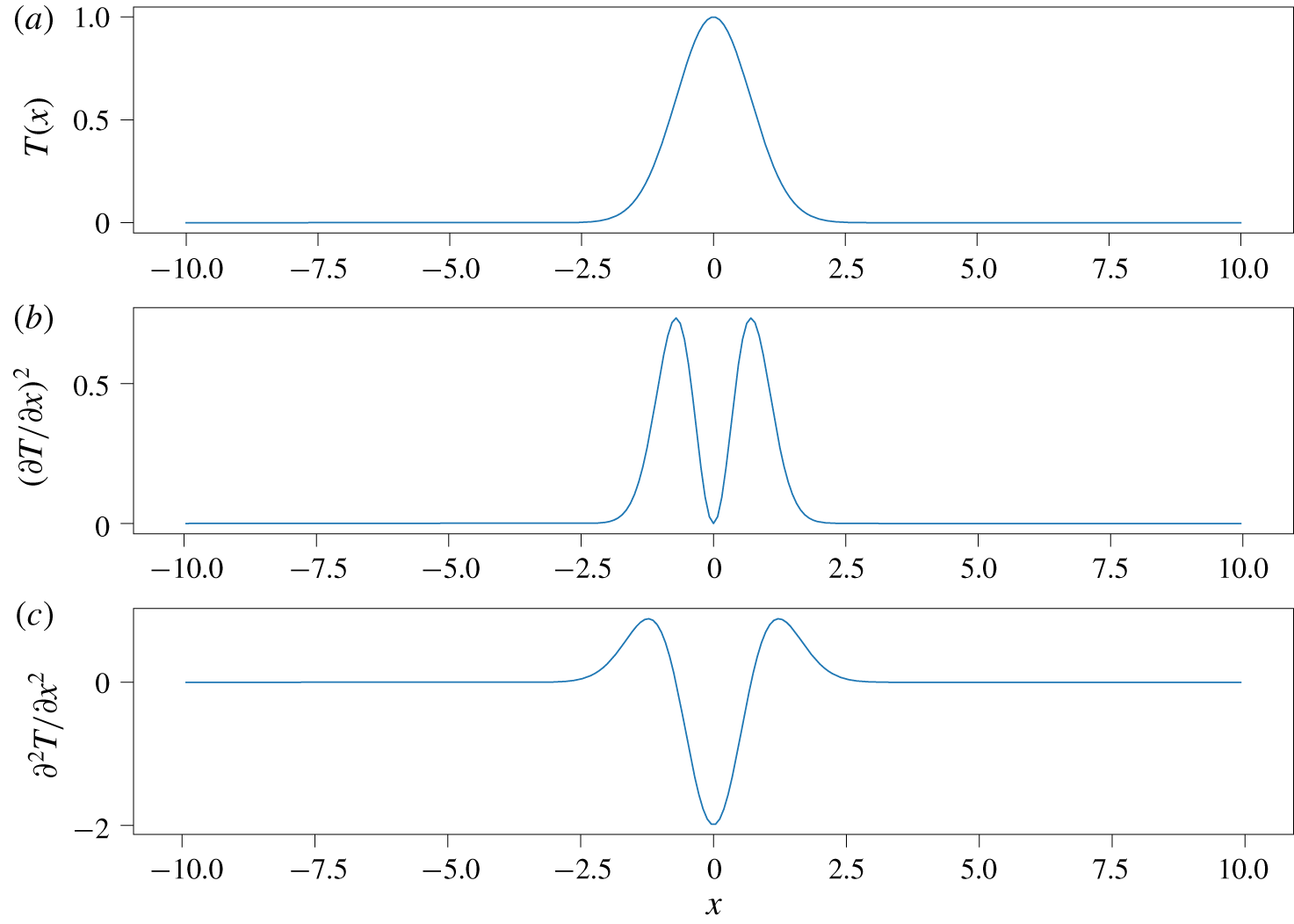
 $\langle \unicode[STIX]{x1D716}_{\unicode[STIX]{x1D703},2D}\rangle _{y}$ in the general case. However, figure 4 sketches the case of a warm fluid parcel over a mostly isothermal background. It is represented by a Gaussian profile for simplicity, but a similar result would be obtained for other bell-shaped curves. The dissipation rate,
 $$\begin{eqnarray}\unicode[STIX]{x1D716}_{\unicode[STIX]{x1D703}}\sim (\unicode[STIX]{x2202}T/\unicode[STIX]{x2202}x)^{2},\end{eqnarray}$$
and the Laplacian,
 $$\begin{eqnarray}\unicode[STIX]{x2202}^{2}T/\unicode[STIX]{x2202}x^{2},\end{eqnarray}$$
have similar shapes, with two maxima located roughly at the warm parcel mid-height.
Simple sketch of patch of hot fluid. (a) Temperature profile. (b) Thermal dissipation profile. (c) Shadowgraph profile.

In the case of the Laplacian, the maxima are positive, and the minimum is negative. This can be observed in both the experimental and numerical shadowgraph images, where a plume pattern consists of darker and lighter boundaries (see figures 2 and 3). The thermal dissipation rate is always positive, and more closely resembles the shadowgraph local variance (discussed in the next section). The qualitative conclusion is that the structures evidenced in the shadowgraph images correspond to both areas of high thermal dissipation rate marking out the plume, which could also be used as a criterion to detect thermal plumes (Belkadi Reference Belkadi2019).
To estimate the similarity of the local variance of the shadowgraph image (figure 3b) and the  $y$-averaged thermal dissipation,
 $\langle \unicode[STIX]{x1D716}_{\unicode[STIX]{x1D703},2D}\rangle _{y}$ (figure 3c), one can compute the time-averaged cross-correlation,
 $C(x,z)$,
 $$\begin{eqnarray}C(x,z)=\frac{\langle S(x,z,t)D(x,z,t)\rangle _{t}-\langle S(x,z,t)\rangle \langle D(x,z,t)\rangle _{t}}{(\langle S(x,z,t)^{2}\rangle _{t}-\langle S(x,z,t)\rangle _{t}^{2})^{1/2}\times (\langle D(x,z,t)^{2}\rangle _{t}-\langle D(x,z,t)\rangle _{t}^{2})^{1/2}},\end{eqnarray}$$
where  $S(x,z,t)$ is the local variance of the shadowgraph, and
 $D(x,z,t)$ is the
 $y$-averaged thermal dissipation. As shown in figure 3d, the cross-correlation is higher than 60 % almost everywhere in the cell, and it averages to 63.8 %. This shows that the two fields are indeed correlated.
4 Spatio-temporal diagrams
4.1 Plume detection technique
Spatio-temporal diagram of the shadowgraph intensity  $I(x,z_{0},t)$. Experimental diagrams at
 $Ra=5.6\times 10^{10}$: (a)
 $z_{0}=5~\text{cm}$ (bottom), (b)
 $z_{0}=20.75~\text{cm}$, (c)
 $z_{0}=36.5~\text{cm}$ (top). Numerical diagrams at
 $Ra=2\times 10^{9}$: (d)
 $z_{0}=4.8~\text{cm}$ (bottom), (e)
 $z_{0}=20~\text{cm}$, (f)
 $z_{0}=35~\text{cm}$ (top). The
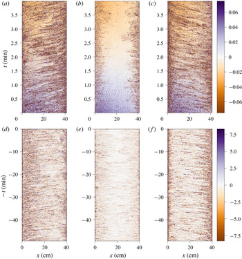
 $t$ axis of the numerical shadowgraph is reversed to visually match the experimental diagrams where the roll direction is opposite.

One common way to find advected structures in a sequence of images is to build a spatio-temporal diagram,  $I(x,z_{0},t)$, by choosing a vertical position
 $z_{0}$, or
 $I(x_{0},z,t)$, by choosing a horizontal position
 $x_{0}$ and plotting the image intensity as a function of
 $x$ and
 $t$, respectively
 $z$ and
 $t$. As shown in figure 5, advected coherent structures yield inclined lines. Similarly to other such analyses in Rayleigh–Bénard convection (Chillà et al. Reference Chillà, Ciliberto, Innocenti and Pampaloni1993; Taberlet et al. Reference Taberlet, Plihon, Auzémery, Sautel, Panel and Gibaud2018), these lines are a clear evidence of the mean wind, in opposite directions near each plate, with no clear advection at the centre.
By measuring the slope of those segments, one can get estimates for the average horizontal velocity (respectively the vertical velocity), and a density of plumes. This method is very common in the field of geophysical fluid dynamics, where it is used to find propagating wave fronts, and is sometimes referred to as a Hovmöller diagram (Lovegrove, Read & Richards Reference Lovegrove, Read and Richards2000; Flór, Scolan & Gula Reference Flór, Scolan and Gula2011).
In the remainder of the paper, we use the terms plume velocity to refer to velocities obtained from the analysis of plume advection (shadowgraph spatio-temporal diagrams, or ‘time-of-flight’ correlation time from thermometers), and fluid velocity to refer to either the numerical simulation velocity field, or experimental PIV measurements.
To obtain a spatio-temporal diagram that can be further successfully post-processed, the contrast of the image must first be enhanced, so that plumes are more visible. The ultimate contrast would consist of texture segmentation, where pixels that belong to a plume are separated from pixels that belong to the bulk. One possible estimate for this type of task is based on the local variance and the local regularity (Pascal et al. Reference Pascal, Pustelnik, Abry, Serres and Vidal2018).
A local variance image is obtained from a standard deviation filtering operation, which consists of computing a new image where each pixel is the standard deviation of the neighbourhood around the corresponding pixel in the original image. High values in this new image correspond to areas where there are large changes in the original image intensity. Low values correspond to areas where the original image intensity is more homogeneous. Hence, boundaries of plumes where there are sharp temperature gradients will produce high local variance values.
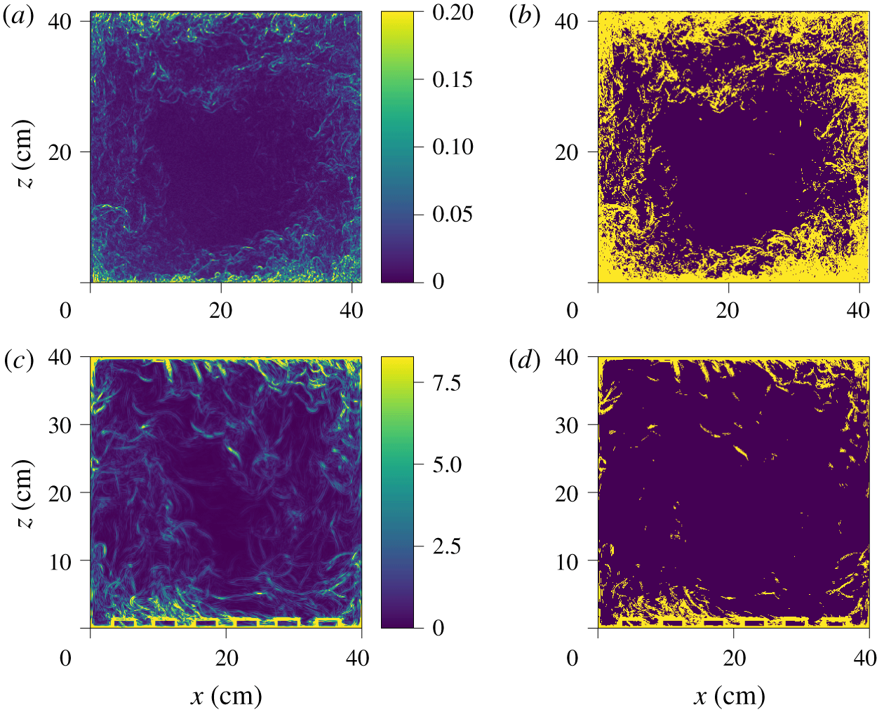
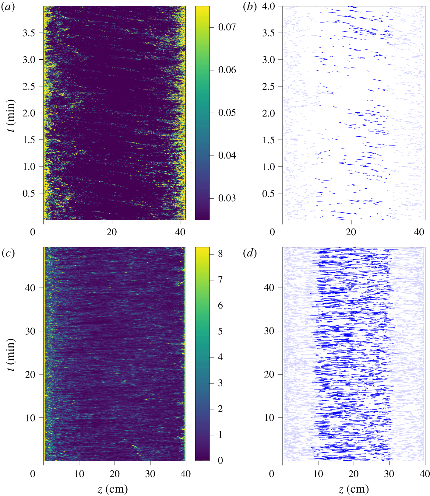
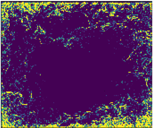
Figure 6(a,c) shows the local variance of the shadowgraph image, computed in neighbourhoods of  $3\times 3~\text{pixels}$, both for the experimental shadowgraph and for the numerical shadowgraph. The contrast is indeed well enhanced.
Local spatial variance of the shadowgraph images shown in figure 2, computed in a neighbourhood of  $3\times 3~\text{pixels}$, for the experimental image at
 $Ra=5.6\times 10^{10}$ (a), and for the numerical shadowgraph at
 $Ra=2\times 10^{9}$ (c). Texture segmentation obtained from thresholding the local variance, (b) for the experimental image with a threshold value 0.025 (in units of relative light intensity), and (d) for the numerical shadowgraph with a threshold value
 $3.1~\text{K}~\text{cm}^{-1}$ (in units of integrated temperature Laplacian).

In the case of the numerical shadowgraph, the resolution is enough to observe the spatial oscillation pattern of each plume. Larger values of neighbourhood would not remove these oscillations, but would lead to blurred images. As previously discussed, they are the result of the double derivative of the spatial temperature profile of the plume (see sketch in figure 4), and should also be visible in the experimental shadowgraph. However, the plumes in the experiments are too small, compared to the resolution of the camera, to fully resolve the structure within each plume, and the oscillation patterns are no longer visible on the local variance image.
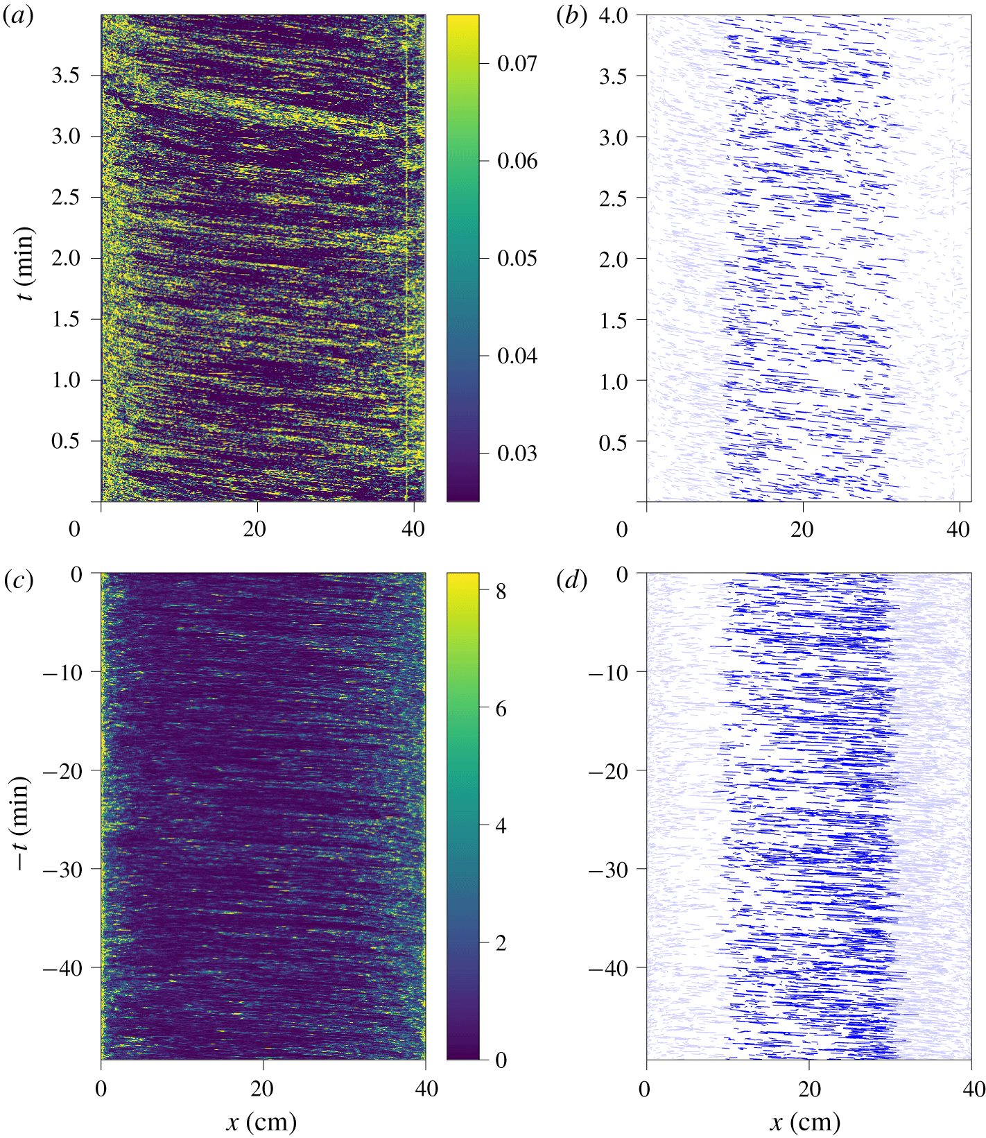
A threshold applied on the local variance yields a segmented picture, where pixels belonging to a plume are separated from those belonging to the bulk. However, in the case of Rayleigh–Bénard convection, the plume density is too high for such a binary decomposition, as can be seen in figure 6(b,d). Therefore, we use the local variance only to enhance the contrast. The spatio-temporal diagrams computed from the local variance images are shown in figure 7 for the case of a horizontal line near the top of the cell, and in figure 8 for the case of a vertical line at  $x_{0}=8~\text{cm}$.
Spatio-temporal diagrams built from the horizontal line at  $z_{0}$ of the local spatial variance shown in figure 6. (a) Experimental diagram at
 $Ra=5.6\times 10^{10}$ for
 $z_{0}=38.5~\text{cm}$ (top). (b) Reconstructed line segments from the experimental diagram, using OpenCV Line Segment Detector. (c) Numerical diagram at
 $Ra=2\times 10^{9}$ for
 $z_{0}=36~\text{cm}$ (top). The
 $t$ axis is reversed to visually match the experimental diagram because the mean wind goes in the opposite direction. (d) Reconstructed line segments from the numerical diagram, using OpenCV Line Segment Detector.

Spatio-temporal diagram built from the vertical line at  $x_{0}=8~\text{cm}$ of the local spatial variance shown in figure 6. (a) Experimental diagram at
 $Ra=5.6\times 10^{10}$. (b) Reconstructed lines from the experimental diagram, using OpenCV Line Segment Detector. (c) Numerical diagram at
 $Ra=2\times 10^{9}$. (d) Reconstructed lines from the numerical diagram, using OpenCV Line Segment Detector.

The experimental and numerical spatio-temporal diagrams are very similar, and also closely resemble the diagrams obtained by Chillà et al. (Reference Chillà, Ciliberto, Innocenti and Pampaloni1993) from the temperature gradient with a sweeping laser method at a lower Rayleigh number ( $Ra=10^{8}$). All feature inclined lines, which are a signature of the advection of plumes.
In the present work, the contrast of the inclined lines is good enough to proceed to the detection of line segments. We use the algorithm of Grompone von Gioi et al. (Reference Grompone von Gioi, Jakubowicz, Morel and Randall2012), implemented in the free OpenCV library (Bradski Reference Bradski2000). The detected segments in the case of a spatio-temporal diagram built from a horizontal line at  $z=z_{0}$, are shown in figure 7(b,d), restricted to segments at the centre of the cell,
 $\unicode[STIX]{x1D709}<x<\ell -\unicode[STIX]{x1D709}$, and with durations
 $\unicode[STIX]{x1D70F}$ of several time steps. For both the experimental and numerical line segments, we choose
 $\unicode[STIX]{x1D709}=\ell /4$, to keep only the contribution of the nearly horizontal wind, and remove the corner flows and the jets. The duration is
 $\unicode[STIX]{x1D70F}=0.4~\text{s}$ for the experimental data, and
 $\unicode[STIX]{x1D70F}=2.3~\text{s}$ for the numerical data. The difference comes from the typical velocity that is much lower in the numerical set-up, due to the lower Rayleigh number.
4.2 Plume density
Each detected segment corresponds to the advection of a thermal plume. However, because some segments are not detected, and because one segment could possibly originate from a group of plumes, the number of detected lines is not directly equal to the number of plumes. Nevertheless, the slope of the detected segments yields an estimate of the plume horizontal velocity,  $U_{x}(x,z_{0},t)$ for diagrams built from horizontal lines at
 $z=z_{0}$, or the plume vertical velocity
 $U_{z}(x_{0},z,t)$ for diagrams built from vertical lines at
 $x=x_{0}$, and the number of detected lines,
 $N_{pl,h}$ and
 $N_{pl,v}$, are estimates of the plume density in both cases.
The detected segments in the case of a spatio-temporal diagram built from a vertical line are shown in figure 8(b,d). In this convention where the origin is at the bottom, we get a positive vertical velocity for  $z\rightarrow 0$, and a negative vertical velocity for
 $z\rightarrow h$. This is a signature of rising plumes at the bottom, and falling plumes at the top. In the case of asymmetrical cells, where only the bottom plate is rough, this analysis allows us to directly compare plume statistics of the smooth and rough plates, with no difference in the optical and image processing parameters.
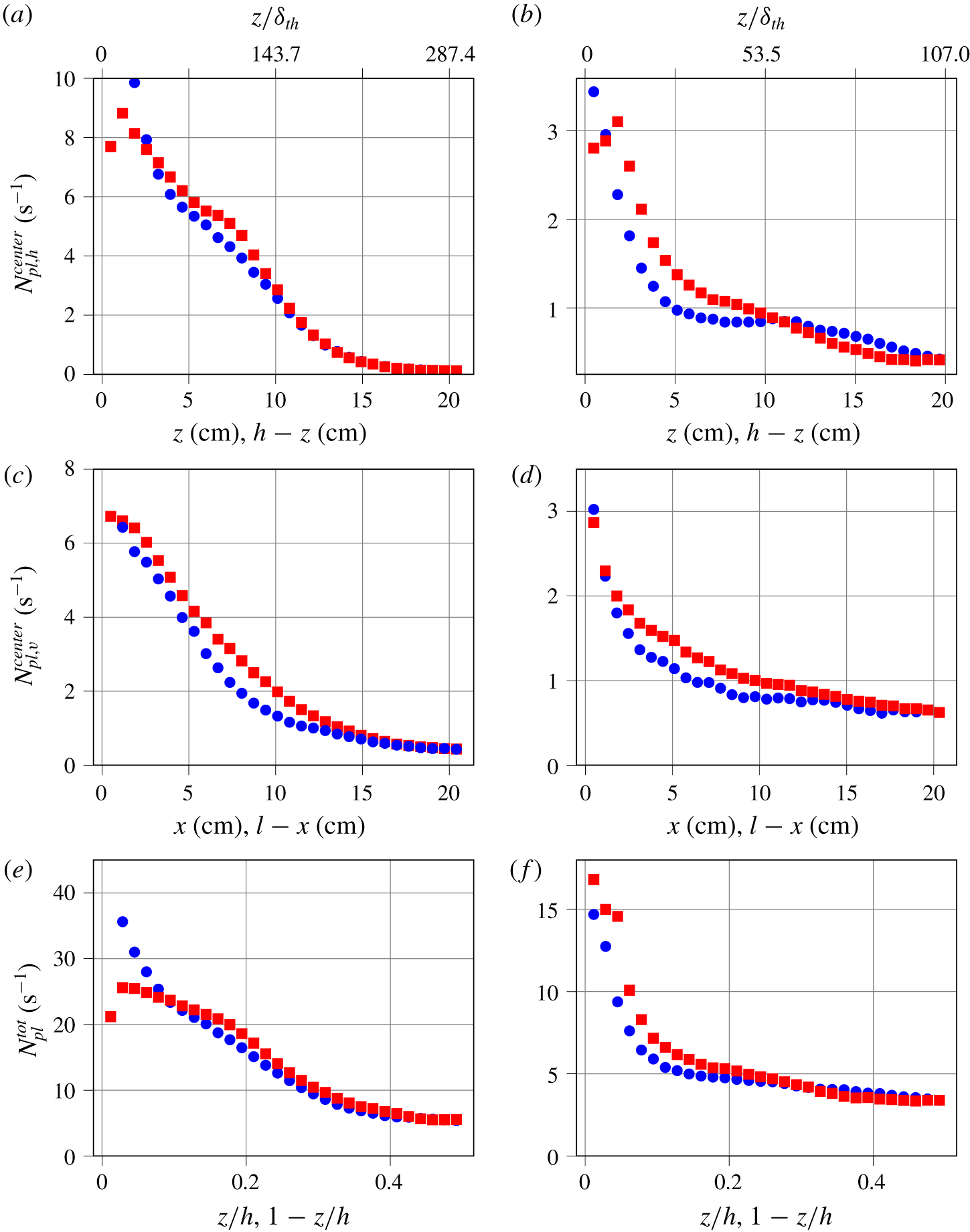
Number of detected segments in the spatio-temporal diagram, per unit time. (a,b) Spatio-temporal diagram from horizontal lines, detecting plumes moving horizontally, as a function of the plate distance  $z$, restricted to the centre area,
 $\unicode[STIX]{x1D709}<x<\ell -\unicode[STIX]{x1D709}$. Blue circles: upper smooth plate. Red squares: lower rough plate. (c,d) Spatio-temporal diagram from vertical lines, detecting plumes moving vertically, as a function of the distance from the wall
 $x$, restricted to the centre area,
 $\unicode[STIX]{x1D709}<z<h-\unicode[STIX]{x1D709}$. Blue circles: falling plumes. Red squares: rising plumes. (e,f) Total number of plumes in the cell, at a given altitude
 $z$. (a,c,e) Experiment at
 $Ra=5.6\times 10^{10}$. (b,d,f) Numerical simulation at
 $Ra=2\times 10^{9}$.

The sets of line segments can be restricted to those at the centre of the cell,  $\unicode[STIX]{x1D709}<x<\ell -\unicode[STIX]{x1D709}$, and
 $\unicode[STIX]{x1D709}<z<h-\unicode[STIX]{x1D709}$, to obtain profiles similar to the kind of profiles found with a probe moving along the axis. We choose
 $\unicode[STIX]{x1D709}/h=1/4$ which is a compromise to have enough events to statistically converge the profile, and is sufficiently away from the walls to be considered nearly at the centre. The resulting number of plumes (per unit time) is shown in figure 9(a–d), for horizontally advected plumes
 $N_{pl,h}^{centre}(z_{0})$, and vertically advected plumes
 $N_{pl,v}^{centre}(x_{0})$.
It is also possible to count the total number of plumes, as a function of plate distance,  $N_{pl}^{tot}(z)$. Indeed, for a vertical line at
 $x=x_{0}$, which yields vertically advected plumes at
 $x=x_{0}$, each detected line segment in the diagram has spatio-temporal coordinates
 $(z_{1},t_{1},z_{2},t_{2})$. One can build the histogram of the space coordinates of their centre positions,
 $N_{pl,v}(x_{0},z)$. The total number of plumes
 $N_{pl}^{tot}$, shown in figure 9(e,f), is
 $$\begin{eqnarray}N_{pl}^{tot}(z)=N_{pl,h}(z)+\mathop{\sum }_{x_{0}}N_{pl,v}(x_{0},z),\end{eqnarray}$$
where  $N_{pl,h}(z)$ is the number of advected plumes on the full horizontal line at
 $z$.
This measurement of the plume density can be compared with predictions and measurements in the literature. In their analysis of the role of plumes in thermal convection, Grossmann & Lohse (Reference Grossmann and Lohse2004) predicted that the number of plumes,  $N_{pl}^{tot}$ scales like
 $$\begin{eqnarray}N_{pl}\sim Nu.\end{eqnarray}$$
In our case, this means that the number of plumes in the experimental case ( $Nu=298.2$) should be three times larger than the number of plumes in the simulation (
 $Nu=107$). As can be seen in figure 9(e,f), for
 $z/h\sim 0.2$, we find indeed approximately 5 plumes per second in the numerical simulation, and 15 plumes per second in the experiment.
One expected effect of plate roughness is to change the emission of thermal plumes. Du & Tong (Reference Du and Tong2000) found that the roughness elements on the plate enhance the detachment of the thermal boundary layer. Although the details of the cell geometry are different in our case, we also previously evidenced bursts of plume emissions near the rough plate, typically between  $40\unicode[STIX]{x1D6FF}_{th}$ and
 $120\unicode[STIX]{x1D6FF}_{th}$ away from the plate, where
 $$\begin{eqnarray}\unicode[STIX]{x1D6FF}_{th}=\frac{H}{2Nu}\end{eqnarray}$$
is the thermal boundary layer thickness (Salort et al. Reference Salort, Liot, Rusaouen, Seychelles, Tisserand, Creyssels, Castaing and Chillà2014).
In the experiment the thermal boundary layer is typically  $\unicode[STIX]{x1D6FF}_{th}\simeq 700~\unicode[STIX]{x03BC}\text{m}$, more than twice smaller than the height of the roughness elements. In this regime, the plate is hydrodynamically rough, and the heat transfer is enhanced.
However, as can be seen in figure 9(a), the average numbers of detected plumes in the present experimental case on the upper and lower halves of the cell only slightly differ. There are more plumes in the range  $50\unicode[STIX]{x1D6FF}_{th}<z<150\unicode[STIX]{x1D6FF}_{th}$, which is where a burst of plumes was previously observed. There are no visible differences far from the plates, when the number of detected plumes vanishes. There seems to be a difference very close to the plate in figure 9(a), with less detected plumes in the rough case. We do not know, at this stage, if our analysis holds so close to the plate, where spurious reflections are possible. We intend to operate a similar experiment on a smooth symmetrical cell to compare. However, further away from the plate, no spurious optical effect is expected. A similar result is obtained from the number of rising and falling plumes in the jets (figure 9c); the number of detected rising plumes is slightly higher than the number of detected falling plumes.
In the numerical simulation, the Rayleigh number is  $Ra=2\times 10^{9}$, and the thermal boundary layer thickness is typically
 $\unicode[STIX]{x1D6FF}_{th}\simeq 1.868~\text{mm}$, almost ten times smaller than the height of the roughness element. Compared to the experimental case, figure 9(b) shows that the plume statistics more strongly differ between the top and the bottom; there are more plumes near the bottom plate. Figure 9(d) shows also that there are more rising plumes than falling plumes.
The stronger plume enhancement observed in the numerical simulation may be a signature of Regime III. Indeed, the experiment lies in Regime II at a relatively high Rayleigh number, and the numerical simulation lies in Regime III, at lower Rayleigh number. In these conditions, the flow is more plume dominated in the numerical simulations than in the experiment, which is more turbulence dominated. It is, however, a general feature that the rough plate yields more total plumes in both cases.
4.3 Velocity statistics
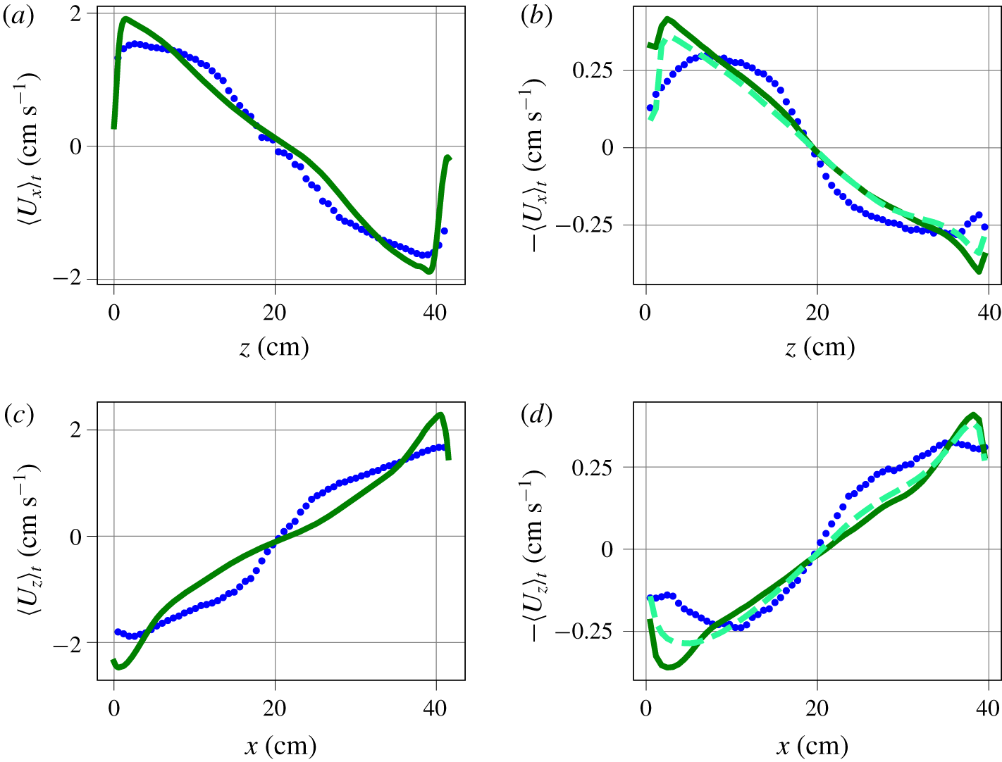
(a,c) Experimental horizontal (respectively vertical) velocity profile, obtained from the slope of the shadowgraph spatio-temporal diagram segments at  $Ra=5.6\times 10^{10}$ (blue circles), or from PIV at
 $Ra=6.2\times 10^{10}$ (solid dark green line). (b,d) Numerical horizontal (respectively vertical) velocity profile, obtained from the slope of the numerical shadowgraph spatio-temporal diagram segments at
 $Ra=2\times 10^{9}$ (blue circles), from the mid-plane slice of the horizontal velocity average (solid dark green line), from the
 $y$-integrated horizontal velocity average (dashed light green line). The
 $\langle U_{x}\rangle$ and
 $\langle U_{z}\rangle$ axes of the simulation are reversed to visually match the experimental profile, where the roll direction is opposite. The average is both temporal and spatial for
 $\unicode[STIX]{x1D709}<x<\ell -\unicode[STIX]{x1D709}$ (respectively
 $\unicode[STIX]{x1D709}<z<h-\unicode[STIX]{x1D709}$), and
 $\unicode[STIX]{x1D709}=\ell /4$ (respectively
 $\unicode[STIX]{x1D709}=h/4$).

The analysis of the segments in the spatio-temporal diagram built from horizontal lines at  $z=z_{0}$ yields sets of plume horizontal velocities,
 $U_{x}(x,z_{0},t)$. From these sets, one can infer the average horizontal velocity,
 $\langle U_{x}\rangle _{t,x}(z_{0})$, as a function of the plate distance, see figure 10(a,b). The average is both temporal and spatial, but only lines near the centre
 $\unicode[STIX]{x1D709}<x<\ell -\unicode[STIX]{x1D709}$ are considered. In the experiment, these profiles can be compared to velocity profiles previously obtained from PIV in similar conditions, and an identical geometry. In the numerical simulation, we use the average velocities of the mid-plane, at
 $y=10~\text{cm}$, as a reference.
These velocity profiles can be compared to those found by Belmonte, Tilgner & Libchaber (Reference Belmonte, Tilgner and Libchaber1994) and Vasiliev et al. (Reference Vasiliev, Sukhanovskii, Frick, Budnikov, Fomichev, Bolshukhin and Romanov2016) in a smooth Rayleigh–Bénard cell filled with water, where the velocity was measured with a pH dye technique. They found a maximum for the velocity at  $z/h\simeq 0.05$, i.e. at
 $z>\unicode[STIX]{x1D6FF}_{th}$. Although our full cell images, either shadowgraph or PIV, do not have the resolution to accurately measure at the scale of boundary layer, similar maxima can be observed in our profiles, and at similar
 $z$.
Similarly, the analysis of the segments of the spatio-temporal diagram built from the vertical lines at  $x=x_{0}$ yields sets of plume vertical velocities,
 $U_{z}(x_{0},z,t)$. From these sets, one can infer the average vertical plume velocity
 $\langle U_{z}\rangle _{t,z}(x_{0})$, as a function of the distance from the wall, see figure 10(c,d).
The plume velocity profiles, obtained from spatio-temporal diagrams or from fluid velocity measurement (PIV in experiment, mid-plane velocity in numerical simulation), have a similar order of magnitude. It is of the order of  $2~\text{cm}~\text{s}^{-1}$ in the experiment, and
 $0.4~\text{cm}~\text{s}^{-1}$ in the numerical simulation. But the profiles do not completely collapse.
We use the numerical simulation to determine if this observed discrepancy is the consequence of the shadowgraph method, rather than an actual difference between plume velocities and fluid velocity. In principle, a difference between average plume velocity and average fluid velocity is not unphysical. Indeed, there is a selection bias; while the advection velocity of a plume should indeed be the same as the local velocity of the fluid, statistics based on plume advection measurements do not account for velocities of fluid parcels between plumes, or in areas where there is no plume. Additionally, the velocity field is divergence free, so a fluid parcel moving up (respectively down) must induce that there is fluid moving down (respectively up). This down-moving fluid parcel is not necessarily a falling plume, as it is moving down because of incompressibility and not because it is colder. The fluid velocity average accounts for all fluid movements, while the plume velocity statistics only account for the contribution of plumes.
Yet, the integration along the  $y$ axis could lower the average, as fluid parcels slowed by the drag on the vertical walls will contribute to the integral. Integration may also smooth larger velocity events. Therefore, to check this hypothesis, we compute a profile of the
 $y$-averaged horizontal fluid velocity. This is similar to what we would get if PIV were integrated in the same manner as the shadowgraph is. This profile is shown in light green dashed line in figure 10(b). As expected, it is slightly lower than the profile obtained without integration in the
 $y$ direction. However, it does not differ from the non-integrated fluid velocity as much as the plume velocity does. This indicates that the integration along
 $y$ is not responsible for the observed difference between the plume velocity average and the fluid velocity average.
It is very broadly assumed in the literature that the velocity of advected plumes can be a satisfactory estimate for the velocity of the ‘wind’, which is then used to infer a Reynolds number. In practice, this is used mostly in cases where direct velocity measurement is not possible, using the correlation time between thermometers in the rising (or falling) jets (Wu Reference Wu1991; Chavanne et al. Reference Chavanne, Chillà, Chabaud, Castaing and Hébral2001; Sun & Xia Reference Sun and Xia2005; He et al. Reference He, van Gils, Bodenschatz and Ahlers2015; Musilová et al. Reference Musilová, Králik, Mantia, Macek, Urban and Skrbek2017), or correlation of shadowgraph images (Funfschilling & Ahlers Reference Funfschilling and Ahlers2004; Brown, Funfschilling & Ahlers Reference Brown, Funfschilling and Ahlers2007). While we find that the average plume velocity yields indeed the same order of magnitude as that of the mean fluid velocity, this analysis shows that care must be taken when comparing the Reynolds numbers computed in this fashion between different cells. He & Tong (Reference He and Tong2011) have analysed the temperature correlation in homogeneous convection. Their result is in agreement with predictions from He & Zhang (Reference He and Zhang2006), and showed that estimates of velocity can be inferred. However, to interpret this velocity estimate properly, there is an underlying assumption that the plume velocity statistics and local velocity statistics are identical. Besides the present work, we are not aware of another direct comparison in the literature between the statistics of plume advection velocity versus local fluid velocity.
In particular, the velocity estimate from rising (or falling) plumes in the jets very close to the walls is close to the maximum fluid velocity, yet still lower. Further away from the wall, average plume velocities are found to be higher than the average fluid velocity. Assuming the velocity profiles shown in figure 10(c) bear some universality, let us discuss the consequence for those results in the literature. They are all performed in cylindrical cells. Let us note by  $\unicode[STIX]{x1D6F7}$ their diameter, and
 $r$ the distance from the wall. Wu (Reference Wu1991) and Musilová et al. (Reference Musilová, Králik, Mantia, Macek, Urban and Skrbek2017) have thermistors at a lateral position
 $r/\unicode[STIX]{x1D6F7}=0.05$, He et al. (Reference He, van Gils, Bodenschatz and Ahlers2015) have thermistors at a lateral position
 $r/\unicode[STIX]{x1D6F7}\sim 0.013$. For those, the plume velocity may be 40 % smaller than the fluid velocity, at least in this range of Rayleigh numbers. Chavanne et al. (Reference Chavanne, Chillà, Chabaud, Castaing and Hébral2001) have thermistors at a lateral position
 $r/\unicode[STIX]{x1D6F7}=0.25$, where plume velocity is slightly larger than average fluid velocity, but the fluid velocity is more than twice smaller than the velocity closer to the walls.
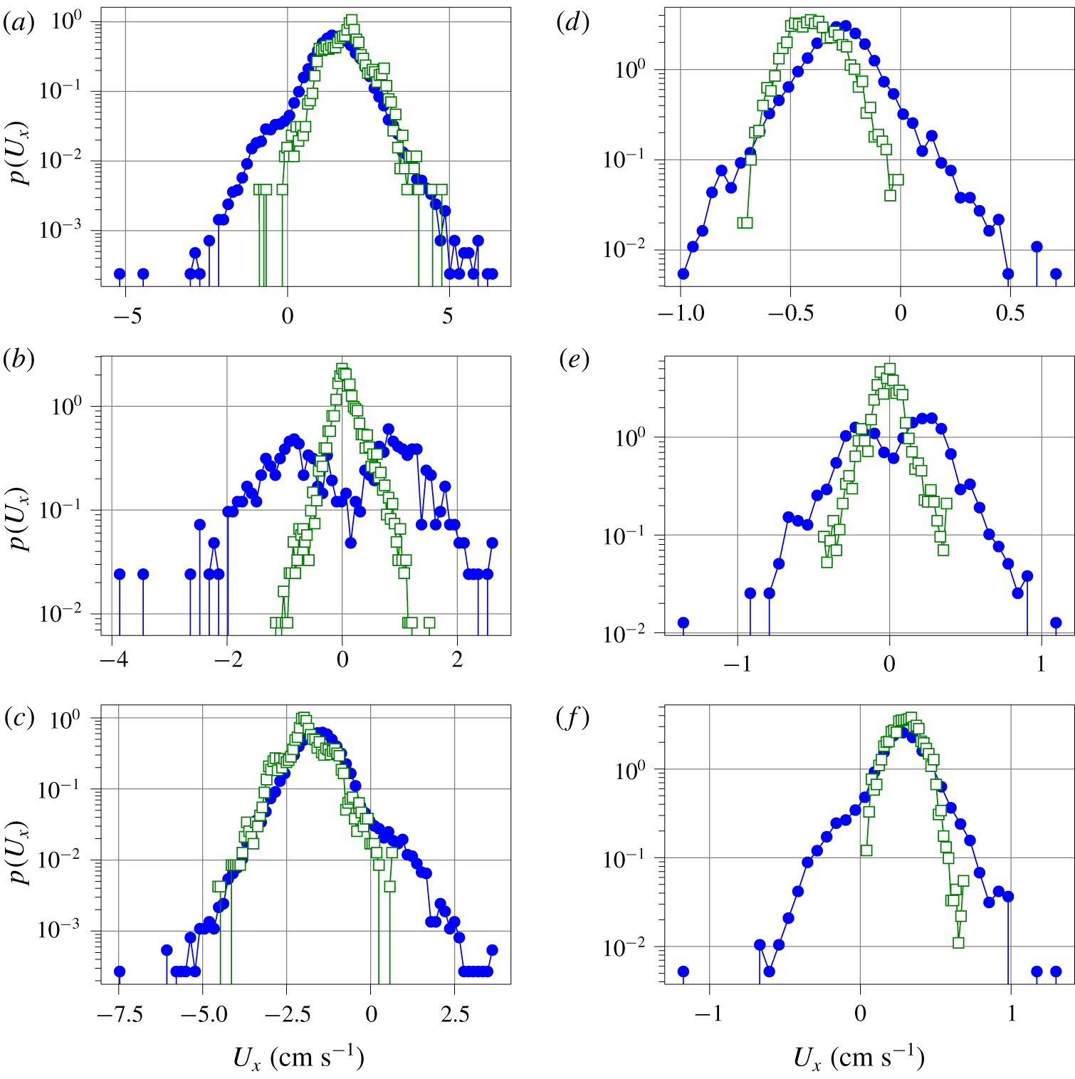
Velocity PDF computed from the shadowgraph spatio-temporal diagram lines (full circles), from PIV measurements for the experimental data or the horizontal velocity mid-plane slice for the numerical simulation (open squares). Experimental data at  $Ra=5.6\times 10^{10}$: (a) 5 cm above the bottom plate. (b) Mid-height. (c) 5 cm below the top plate. Numerical simulations at
 $Ra=2\times 10^{9}$: (d) 5 cm above the bottom plate. (e) Mid-height. (f) 5 cm below the top plate.

Finally, the velocity probability density functions (PDFs) are shown in figure 11. The PDFs of the experimental and numerical data are mostly similar.
The velocity PDF, obtained from the fluid velocity (PIV measurements in the experiment, mid-plane velocity in the numerical simulation), and those obtained from the shadowgraph spatio-temporal diagram, are similar at  $z=5~\text{cm}$ and
 $z=35~\text{cm}$. However, they seem to evidence exponential tails which may seem to be in contradiction with the data from Qiu et al. (Reference Qiu, Shang, Tong and Xia2004) in a cylindrical cell, or Belmonte et al. (Reference Belmonte, Tilgner and Libchaber1994) in a cubic cell, where Gaussian velocity PDFs are measured at the centre of the convection cell. But Zhou, Sun & Xia (Reference Zhou, Sun and Xia2007b) report an exponential velocity PDF, away from the sidewalls in a rectangular cell, with a geometry much closer to ours. The difference between cylindrical and cubic versus rectangular may arise from the contribution of azimuthal motion which is reported to have a Gaussian amplitude PDF (Xi, Zhou & Xia Reference Xi, Zhou and Xia2006).
In the experiment, small differences in the operating conditions (see table 1) could account for the slight differences. Some velocity PDFs obtained from PIV exhibit secondary peaks (clearly visible for example in figure 11(c), at  $z\approx -2~\text{cm}~\text{s}^{-1}$ and
 $z\approx -3~\text{cm}~\text{s}^{-1}$). These velocities are close to integer pixel displacements and are due to peak locking, which are known artefacts of the sub-pixel estimator used by the PIV algorithm Raffel et al. (Reference Raffel, Willert, Wereley and Kompenhans1998).
The PDFs are, however, very different at the centre of the cell, where the fluid velocity exhibits a symmetric histogram centred on zero, while the plume velocity PDFs evidence two peaks. The reason is that our method can only capture advected plumes, in one direction or another, but cannot resolve vanishing velocities, where no plume is advected.
The plume velocity histograms always evidence events in both directions ( $U_{x}>0$ and
 $U_{x}<0$), but the most probable plume velocity value matches the most probable fluid velocity. The plume velocity distributions at
 $z=5~\text{cm}$ and
 $z=35~\text{cm}$ are slightly skewed, which may be a signature of the two kinds of plumes that are captured; plumes emitted from the top plate and those emitted from the bottom plate, which each have their PDF. The final PDF is the superposition of the PDFs of these two kinds of plumes.
5 Conclusions
We have shown that synthetic shadowgraph images can be computed in numerical simulations from the full temperature field, and that they are strikingly similar to experimental shadowgraph images. This confirms that simple geometrical optics is a sufficient model for shadowgraphy in Rayleigh–Bénard convection. The contrast of the shadowgraph image can be greatly enhanced by computing the local variance of the image. Although there is no straightforward analytical relation, the DNS images show that this local variance shadowgraph image closely resembles the local thermal dissipation rate.
The local variance shadowgraph allows us to build high contrast spatio-temporal diagrams, and opens the way to automatic detection of line segments. Statistics of thermal plumes can be inferred from these sets of line segments. The velocity estimated from the slope of these segments, and interpreted as the plume velocity, has the same order of magnitude as the fluid mean velocity, but they are not identical, with a relative difference of up to 40 %. This is important because advected plume times of flight are widely used as estimates for the ‘wind’ velocity, when direct velocity measurement is not possible. Additionally, other statistics such as the plume velocity PDF, may differ from the fluid velocity PDF, so one must exert caution when inferring higher-order statistics.
The analysis of the plume density, in Rayleigh–Bénard cells with a rough bottom plate and a smooth top plate, shows direct evidence of the increase of plume emission, as well as possible signatures of the transition between the roughness-triggered plume-dominated regime and the roughness-triggered turbulent regime. In this asymmetric configuration, the number of rising hot plumes is larger than the number of falling cold plumes.
Acknowledgements
This numerical work was granted access to the HPC resources of GENCI-IDRIS under allocation 2a0326 made by GENCI. The experimental work benefited from funding by ANR-18-CE30-0007-01 JCJC ‘CryoGrad’ project. The experiments could not have been possible without the help of M. Moulin and the mechanical workshop who designed and built the experimental cell. The collaborative work between Limsi and LPENSL was funded by the CNRS INSIS PEPS Energie 2018 ‘CORINThe’ joint project. Image processing benefited from the resources of the PSMN computing centre in Lyon.
The authors are grateful to B. Pascal and N. Pustelnik for an interesting discussion about image segmentation, and for suggesting to compute the local variance. We thank B. Castaing, D. Dumont and L. Méthivier for proofreading of this manuscript.
Declaration of interests
The authors report no conflict of interest.