1. Introduction
As a problem of great value in practical applications, the turbulent boundary layer (TBL) has attracted the attention of researchers since the boundary layer was proposed by Prandtl in 1904. Since turbulence consists of random velocity fluctuations, studying the interactions between fluctuations and the mean flow based on Reynolds decomposition (Reynolds Reference Reynolds1895) is an important strategy for understanding TBLs. In comparison with the zero-pressure-gradient (ZPG) cases (Pope Reference Pope2000; Panton Reference Panton2005, Reference Panton2007; Marusic et al. Reference Marusic, McKeon, Monkewitz, Nagib, Smits and Sreenivasan2010), the effects of the adverse pressure gradient (APG) penetrate deep into different regions of TBLs and cause more complex interactions. The present work focuses on the behaviour of turbulence production in TBLs over a wide range of pressure gradients from ZPG to separation. Turbulence production here can be derived from both the mean flow energy equation and the turbulent energy budget equation (Tennekes & Lumley Reference Tennekes and Lumley1972) and can be expressed as
 \begin{equation} {\mathscr {P}}=-\overline {{{u}_{i}}{{u}_{j}}}{{S}_{ij}},\text { }{{S}_{ij}}=\frac {1}{2}\left(\frac {\partial {{u}_{i}}}{\partial {{x}_{j}}}+\frac {\partial {{U}_{j}}}{\partial {{x}_{i}}}\right), \end{equation}
where
 ${u}_{i}$
denotes the fluctuating velocity components,
 ${S}_{ij}$
is the mean rate of strain and
 ${u}_{i}$
denotes the mean velocity components.
Various studies (e.g. Pope Reference Pope2000; Wei Reference Wei2018) on the ZPG have revealed the unique value of turbulence production in terms of mean flow and fluctuation properties. For example, the peak of turbulence production appears in the viscous buffer layer, and the position of the peak does not vary with the Reynolds number (Fernholz & Finley Reference Fernholz and Finley1996; She et al. Reference She, Chen and Hussain2017; Cantwell Reference Cantwell2019). This phenomenon accounts for the dramatic energy exchange between the mean flow and turbulence in the viscous buffer layer. The term ‘dramatic’ used in this paper to describe the degree of energy exchange specifically refers to a degree that is sufficient to cause a peak of turbulence production. The gradually active turbulent motion in the viscous buffer layer combined with the non-negligible viscous stress also contributes to the difficulty in predicting the mean velocity. In contrast, the overlapping region above the viscous buffer layer is thought to be in a local equilibrium where turbulence production equals dissipation (Tennekes & Lumley Reference Tennekes and Lumley1972; Pope Reference Pope2000), and a well-known log law is obtained here by matching the mean velocities in the inner and outer regions (Isakson Reference Isakson1937; Millikan Reference Millikan1938). The peak value of turbulence production is also found to be constant under different Reynolds numbers due to the equal stress layer, i.e.
 $\mathscr {P}^{+}={\mathscr {P}}/(u_{\tau }^{4}/\nu )=1/4$
, where the superscript
 $+$
denotes viscous units,
 $u_\tau =\sqrt {\tau _w/\rho }$
is the wall friction velocity and
 $\tau _w$
is the wall shear stress. Taking advantage of properties of the peak value, Chen & Sreenivasan (Reference Chen and Sreenivasan2021) proposed a growth process of
 $\overline {uu}$
peaks different from that of Marusic, Baars & Hutchins (Reference Marusic, Baars and Hutchins2017). Moreover, formulations for the bounded dissipation of turbulent fluctuations were developed on this basis (Chen & Sreenivasan Reference Chen and Sreenivasan2022 Reference Chen and Sreenivasan2023). Renard & Deck (Reference Renard and Deck2016) derived a decomposition of the mean skin friction coefficient based on the turbulent energy budget. The decomposition holds for the ZPG and APGs, where turbulence production is identified as a localised source causing the mean friction. This decomposition was further applied to seven APG databases by Fan et al. (Reference Fan, Li, Atzori, Pozuelo, Schlatter and Vinuesa2020). Their results show that as the APG coefficient increases, the component of turbulence production significantly increases and becomes dominant for the mean friction.
For APGTBLs, turbulence production plays a more significant role due to the increase in turbulence intensity and the energy exchange between mean flow and turbulence. Townsend (Reference Townsend1961) proposed a structural parameter between turbulent kinetic energy and Reynolds shear stress and assumed a linear stress layer different from the ZPG to predict the mean velocity. Bradshaw, Ferriss & Atwell (Reference Bradshaw, Ferriss and Atwell1967) adopted this structural parameter and transformed the turbulent energy balance equation into a turbulent shear stress equation to calculate boundary layer development. Furthermore, one of the most widely used turbulence models, the Menter shear-stress transport turbulence model (Menter Reference Menter1994), imposes a limiter on turbulence production by introducing the Bradshaw assumption. The application of this limiter has led to significant improvements in the accuracy of predictions of APG and separated flows (Menter Reference Menter1994; Menter, Kuntz & Langtry Reference Menter, Kuntz and Langtry2003). Other researchers (Allamaprabhu, Raghunandan & Morinigo Reference Allamaprabhu, Raghunandan and Morinigo2011; Georgiadis & Yoder Reference Georgiadis and Yoder2013; Xu, Zhang & Bai Reference Xu, Zhang and Bai2015; Kalitzin, Medic & Xia Reference Kalitzin, Medic and Xia2016; Raje & Sinha Reference Raje and Sinha2021; Bai et al.. Reference Bai, Ma, Zhang, Jiang and Yan2023; Song et al. Reference Song, Ma, Yi, Shao, Bai and Yan2024) have also focused on the value of turbulence production for the prediction of APG flows. Therefore, studying the behaviour of turbulence production in APG TBLs not only contributes to our understanding of TBLs but also helps to improve the accuracy of turbulence simulations.
Another reason why turbulence production is important in APG TBLs is active large-scale outer-region motions. Various recent studies of coherent structures (Rahgozar & Maciel Reference Rahgozar and Maciel2011; Monty, Harun & Marusic Reference Monty, Harun and Marusic2011; Harun et al. Reference Harun, Monty, Mathis and Marusic2013) have pointed to an increase in the number or intensity of large-scale motions. In terms of statistical properties, turbulent fluctuations are enhanced with the injection of energy from the pressure gradient (Nagano, Tagawa & Tsuji Reference Nagano, Tagawa and Tsuji1992; Spalart & Watmuff Reference Spalart and Watmuff1993; Krogstad & Skåre Reference Krogstad and Skåre1995; Marusic & Perry Reference Marusic and Perry1995; Skote & Henningson Reference Skote and Henningson2002), and statistical quantities including the Reynolds shear stresses show a tendency for the peak position to be shifted outward (Kitsios et al. Reference Kitsios, Sekimoto, Atkinson, Sillero, Borrell, Gungor, Jimnez and Soria2017; Maciel et al. Reference Maciel, Wei, Gungor and Simens2018). For turbulence production, the APG causes a much larger near-wall production peak (inner peak) (Bobke et al. Reference Bobke, Vinuesa, Örlü and Schlatter2016, Reference Bobke, Vinuesa, Örlü and Schlatter2017) and a gradual apparent outer peak that is significantly different from that in the ZPG case (Bobke et al. Reference Bobke, Vinuesa, Örlü and Schlatter2017; Kitsios et al. Reference Kitsios, Sekimoto, Atkinson, Sillero, Borrell, Gungor, Jimnez and Soria2017; Coleman, Rumsey & Spalart Reference Coleman, Rumsey and Spalart2018). The position of the inner peak is also no longer fixed as in the ZPG TBL but becomes closer to the wall as the pressure gradient increases (Kitsios et al. Reference Kitsios, Sekimoto, Atkinson, Sillero, Borrell, Gungor, Jimnez and Soria2017). Gungor, Maciel & Gungor (Reference Gungor, Maciel and Gungor2022) compared the spectral distributions of production in small-defect and large-defect APG TBLs and found that an increase in the velocity defect had no significant effect on the distributions. Rkein & Laval (Reference Rkein and Laval2023) generated a direct numerical simulation (DNS) database of high Reynolds numbers for moderate APGs where the APG allows a clear outer peak to be present. For moderate APGs, the main difference between the Reynolds stress budget and that of the ZPG TBL is a significant production and dissipation in the outer region. However, our understanding of the values and positions of the two peaks remains at a qualitative stage. According to a review of studies on different physical quantities, energy-containing structures and turbulence models, quantitatively investigating the bimodal behaviour is one of the keys to a deeper understanding of energy change and transfer. Combined with the non-variation of the value and position of the turbulence production peak in the ZPG TBL, it also becomes attractive to try to predict a certain invariance of the bimodal peaks of turbulence production in APG TBLs.
The remainder of this paper is organised as follows: § 2 introduces the databases used in this paper and their basic information. Section 3 illustrates the changes in peaks and components of turbulence production in APG TBLs, which are the focus of attention later on. Sections 4 and 5 investigate the inner and outer peaks through different length scale ratios and time scale ratios, respectively. On this basis, we analyse the behaviour of turbulence production in relation to the mean flow and give specific predictions for the position and value of the inner peak. Conclusions are provided in § 6.
2. The APG databases
We expect the selected databases to satisfy the following requirements: they should encompass a wide range of pressure gradients from ZPG to separation; include both equilibrium and non-equilibrium flows; cover moderate Reynolds numbers and high Reynolds numbers. The requirement for the Reynolds numbers is not merely expected to extend the range of Reynolds numbers. It also takes into account that, from the asymptotic perspective, the effects of Reynolds numbers and pressure gradients somewhat restrain each other (Panton Reference Panton2005; Afzal Reference Afzal2008; Scheichl & Kluwick Reference Scheichl and Kluwick2013), resulting in flows corresponding to the same pressure gradient parameter possibly differing significantly. Therefore, comparing pressure gradient effects without considering Reynolds numbers has considerable limitations. Eleven databases are used to validate our ideas, including one non-equilibrium experimental database from Cuvier et al. (Reference Cuvier2017), five equilibrium large-eddy simulation (LES) databases from Bobke et al. (Reference Bobke, Vinuesa, Örlü and Schlatter2017), two equilibrium DNS databases from Kitsios et al. (Reference Kitsios, Sekimoto, Atkinson, Sillero, Borrell, Gungor, Jimnez and Soria2017) and three non-equilibrium DNS databases from Coleman et al. (Reference Coleman, Rumsey and Spalart2018), Coleman (Reference Coleman2021) and Rkein & Laval (Reference Rkein and Laval2023). Since the method used in the inner region in this paper involves second-order derivatives, its validation on the experimental data we have is not available temporarily.
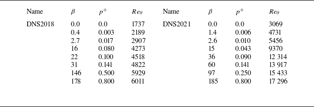
Basic information on the selected databases is listed in table 1. The reference Reynolds number is defined by the boundary layer edge velocity
 $U_{e}$
and the momentum thickness
 $\theta$
. Two defined forms of pressure gradient parameters are given,
 $p^{+}=(v{\rm d}P_w/{\rm d}x)/(\rho {u}^3_{\tau })$
and
 $\beta =(\delta ^{*}dP_{e}/{\rm d}x)/(\rho {u}^{2}_{\tau })$
, where
 $\delta ^{*}$
is the boundary layer displacement thickness and
 $P_{e}$
is the potential flow pressure at the edge of the boundary layer. Both pressure gradient parameters are monotonic before separation. We use the
 $p^+$
defined by inner scales to describe flows in this paper. The reason is that we wish to quantitatively explain the self-similar behaviour of the turbulence production and the inner region is usually considered to be self-similar (Tennekes & Lumley Reference Tennekes and Lumley1972).
The APG databases used in this study. The stations chosen in equilibrium databases are presented in brackets.

The two non-equilibrium databases, DNS2018 and DNS2021, both contain the entire APG regions
 $(p^+=0\sim \infty )$
to be studied. They correspond to moderate and high Reynolds number flows, respectively, enabling us to thoroughly examine the research. Additionally, DNS2018 achieved the target of a canonical ZPG state upstream of the APG, which was proven to agree extremely well with the DNS data from that of Schlatter & Örlu (Reference Schlatter and Örlü2010) and can be used for parameter calibration. Two high Reynolds number non-equilibrium databases that correspond to moderate APGs are EXP2017 and DNS203. The DNS2023 database was designed to have approximately the same APG magnitude as EXP2017 (Rkein & Laval Reference Rkein and Laval2023). The two equilibrium DNS databases were realised by keeping the pressure gradient parameters
 $\beta$
unchanged (Kitsios et al. Reference Kitsios, Sekimoto, Atkinson, Sillero, Borrell, Gungor, Jimnez and Soria2017). The mild APG database (DNS2017(b1)) corresponds to moderate Reynolds numbers, and the strong APG database (DNS2017(b39)) corresponds to high Reynolds numbers. The five LES databases achieved equilibrium flows through two different methods (Bobke et al. Reference Bobke, Vinuesa, Örlü and Schlatter2017). The first method was by keeping the self-similarity parameter
 $m=({\delta }{\rm d}U_{e}/{\rm d}x)/(U_{e}{\rm d}{\delta }/{\rm d}x)$
unchanged (LES2017(m13), LES2017(m16) and LES2017(m18)), where
 $\delta$
is the boundary layer thickness. The second method further kept the pressure gradient parameter
 $\beta$
roughly unchanged (LES2017(b1) and LES(b39)). According to the similarity analysis, maintaining a consistent similarity parameter
 $m$
can preserve the self-similarity of the velocity defect (Castillo & George Reference Castillo and George2001; Devenport & Lowe Reference Devenport and Lowe2022), but strict self-similarity requires maintaining consistent pressure gradient parameters (Maciel, Rossignol & Lemay Reference Maciel, Rossignol and Lemay2006). Due to a certain range of changes in
 $\beta$
in the LES databases, they can be regarded as approximate equilibrium flows. The DNS2017(b1) and DNS2017(b39) can be regarded as strict equilibrium flows since they also control standard deviations of other similarity parameters. To avoid duplication, we show only one station from each equilibrium database in the analysis below. Information on the selected stations is presented in brackets in table 1. For DNS2018 and DNS2021, the pressure gradient and Reynolds number details for the reference positions used in this paper are further presented in table 2.
Information about reference stations in DNS2018 and DNS2021.

3. Changes in turbulence production in APG TBLs
Before we start to analyse turbulence production, we first explain the relationship between turbulence production, the mean flow energy equation and the turbulence energy budget equation. This process seems to be a bit repetitive, but it illustrates the unique value of turbulence generation as distinct from turbulent dissipation, turbulent diffusion, turbulent convection and so on. The momentum equation for an incompressible fluid is as follows:
 \begin{equation} \frac {\partial \widetilde {{{u}_{i}}}}{\partial t}+\widetilde {{{u}_{j}}}\frac {\partial \widetilde {{{u}_{i}}}}{\partial {{x}_{j}}}=-\frac {1}{\rho }\frac {\partial \widetilde {p}}{\partial {{x}_{i}}}+2\nu \frac {\partial \widetilde {{{s}_{ij}}}}{\partial {{x}_{j}}} , \end{equation}
where the superscript
 $\sim$
represents the instantaneous value of the physical quantity, that is, the sum of the mean component and the fluctuating component. The steady mean flow motion equation obtained by ensemble averaging (3.1) is
 \begin{equation} {U}_{j}\frac {\partial {{U}_{i}}}{\partial {{x}_{j}}}=-\frac {1}{\rho }\frac {\partial P}{\partial {{x}_{i}}}+\frac {\partial }{\partial {{x}_{j}}}(2\nu {{S}_{ij}}-\overline {{{u}_{i}}{{u}_{j}}})\ . \end{equation}
Multiplying both sides of (3.2) by
 ${u}_{i}$
yields the mean flow energy equation
 \begin{equation} {U}_{j}\frac {\partial }{\partial {{x}_{j}}}\left(\frac {1}{2}{{U}_{i}}{{U}_{i}}\right)=\frac {\partial }{\partial {{x}_{j}}}\left(-\frac {P}{\rho }{{U}_{j}}+2\nu {{S}_{ij}}{{U}_{i}}-\overline {{{u}_{i}}{{u}_{j}}}{{U}_{i}}\right)-2\nu {{S}_{ij}}{{S}_{ij}}+\overline {{{u}_{i}}{{u}_{j}}}{{S}_{ij}} . \end{equation}
Multiplying both sides of (3.1) by
 $\widetilde {{{u}_{i}}}$
, taking the average time of all terms, and subtracting (3.3) yields the turbulent energy budget equation
 \begin{equation} {U}_{j}\frac {\partial }{\partial {{x}_{j}}}\left(\frac {1}{2}\overline {{{u}_{i}}{{u}_{i}}}\right)=-\frac {\partial }{\partial {{x}_{j}}}\left(\frac {1}{\rho }\overline {p{{u}_{j}}}+\frac {1}{2}\overline {{{u}_{i}}{{u}_{i}}{{u}_{j}}}-2\nu \overline {{{u}_{i}}{{s}_{ij}}}\right)-\overline {{{u}_{i}}{{u}_{j}}}{{S}_{ij}}-2\nu \overline {{{s}_{ij}}{{s}_{ij}}}. \ \end{equation}
The first three terms on the right-hand side of (3.3) represent the transport of mean-flow energy by stresses, and the fourth and fifth terms are known as deformation work. One reason for this distinction is that they correspond to two processes in turbulence dynamics: spatial energy transfer and deformation work. The property of ‘transport’ in (3.3) is that the first three terms of the right-hand side can only redistribute energy within the control volume if the part in the brackets on the right-hand side is zero on the surface of a control volume. By conservation of energy, the deformation work represents the mean-flow energy lost, which can also be understood as the mean-flow energy retrieved from the stress-generating agency. The contribution of viscous stresses to the deformation work is always negative, and therefore it is called viscous dissipation of the mean-flow energy. In TBLs,
 $S_{ij}$
and
 $\overline {{{u}_{i}}{{u}_{j}}}$
take on opposing values of positive and negative, so the contribution of Reynolds stresses is also dissipative. The kinetic energy of the turbulence benefits from this work and
 $-\overline {{{u}_{i}}{{u}_{j}}}{{S}_{ij}}$
is called turbulence production for this reason. We get the observation of changes in the mean flow energy from (3.3), but (3.3) is derived merely from a simple transformation of the mean momentum equation and does not contain much more information. The turbulent energy budget described by (3.4) therefore receives more attention.
In (3.4), the turbulence production term also appears along with other terms that describe the characteristics of turbulence fluctuations. The rate of change of the turbulent kinetic energy is related to transport by pressure gradients, transport by turbulent velocity fluctuations, transport by viscous stresses and two kinds of deformation work. Like those in (3.3), the transport terms are divergences of energy flux. They are involved in the redistribution of energy from one point to another. More important are deformation works, which are known as turbulence production and turbulence dissipation. Their variations have been an important concern for the ZPG (Pope Reference Pope2000; Marusic et al. Reference Marusic, McKeon, Monkewitz, Nagib, Smits and Sreenivasan2010) and APG (Bradshaw et al. Reference Bradshaw, Ferriss and Atwell1967; Tennekes & Lumley Reference Tennekes and Lumley1972; Townsend Reference Townsend1976) flows. Turbulence production appears in the opposite sign to the deformation work of Reynolds stresses of (3.3). Turbulent dissipation is the rate at which viscous stresses perform deformation work against the fluctuating strain rate and is always a drain of energy. What makes turbulence production particularly unique compared with turbulence dissipation is its simultaneous appearance in (3.3) and (3.4). This means that turbulence production represents the energy exchange between mean flow and turbulence, which involves a loss from the mean flow and a gain in the turbulence. The position of the most dramatic energy exchange reflects the peak of turbulence production, which severely disrupts the balance between production and dissipation and thus is key to understanding the behaviour of turbulence production. Because of the equal stress layer in the ZPG TBL, it is mathematically possible to obtain the peak value. However, in APG TBLs, not only does an additional peak appear in the outer region of strong APGs, but also the pressure gradient makes the prediction of the peak values difficult. Thus, we first illustrate in this section the changes in turbulence production by the APG for later analysis.
3.1. The bimodal distribution of turbulence production
The bimodal distribution of turbulence production can be recognised qualitatively in terms of the turbulent energy budget. The relationship between turbulence production and turbulence dissipation in the ZPG, especially their local balance within the overlapping region, is crucial for understanding TBLs. The production and the dissipation are also considered to be of the same magnitude. It is still helpful to first focus on the relationship between the two in APG TBLs. As an example, figure 1 compares turbulence production and dissipation in four APG cases of equilibrium and non-equilibrium flows, where the other terms in (3.4) are shown together.
Turbulent energy budget in equilibrium and non-equilibrium APG TBLs. Production,
 $-\overline {{{u}_{i}}{{u}_{j}}}{{S}_{ij}}$
; dissipation,
 $-2\nu \overline {{{s}_{ij}}{{s}_{ij}}}$
; convection, (1/2)
 ${U}_{j}\partial \overline {{{u}_{i}}{{u}_{i}}}/\partial {{x}_{j}}$
; pressure transport,
 $-(1/\rho )\partial \overline {p{{u}_{j}}}/\partial {{x}_{j}}$
; turbulent transport,
 $-(1/2)\partial \overline {{{u}_{i}}{{u}_{i}}{{u}_{j}}}/\partial {{x}_{j}}$
; viscous transport,
 $2\nu \partial \overline {{{u}_{i}}{{s}_{ij}}}/\partial {{x}_{j}}$
. Budget terms normalised by
 $U_e^3/\delta$
. Here (a) DNS2017(b1),
 $p^+=0.006$
; (b) DNS2017(b39),
 $p^+=0.11$
; (c) DNS2018,
 $p^+=0.003$
; (d) DNS2018,
 $p^+=0.800$
.

From the slight APG in figure 1(c) to the moderate APG in figure 1(a) and then to the strong APGs in figures 1(b) and 1(d), production and dissipation always remain of the same order of magnitude. It is noteworthy to observe the changes in local balance in the overlapping region. In the cases of slight and moderate APGs, production still equals dissipation in the overlapping region. However, this balance is disrupted at strong APGs. The excess dissipation is balanced mainly by the turbulent transport term in the overlapping region. Since the APG enhances the turbulence intensity, turbulent transport participates in the balance of production and dissipation. Moreover, the overlapping region is far away from the wall and external flow, and physical processes such as viscous transport and convection can still be neglected. Therefore, a new local balance appears in the overlapping region. As in the ZPG TBL, the local balance allows the derivation of the classical log law. The new local balance also allows the analysis to be simplified in the overlapping region of APG TBLs, thus supporting the existence of self-similarity laws similar to the log law in APG TBLs. Examples include some studies (Townsend Reference Townsend1961; Afzal Reference Afzal2008; Scheichl & Kluwick Reference Scheichl and Kluwick2013; Ma et al. Reference Ma, Bai, Song, Zhang and Yan2024a ) of mean velocity and total stress scalar laws, where a simplified derivation by Townsend (Reference Townsend1961) can be an intuitive understanding. Townsend Reference Townsend1961 assumed the structural parameters of the terms in the turbulence budget equation. Since turbulence production includes the velocity gradient, he further derived the scaling law of the mean velocity from the balance of the turbulence budget terms. The local balance illustrates the important roles of production and dissipation in energy transfer. However, the bimodal peaks of turbulence production are present in the inner region below the overlapping region and the outer region above the overlapping region. The turbulent transport and viscous transport are both non-negligible near the inner peak as well as the pressure transport which becomes significantly larger as the separation approaches. Near the outer peak, the convection cannot be neglected in addition to the turbulent transport. The additional physical processes involved at these locations result in more difficult predictions of turbulent quantities compared with the overlapping region. Establishing a link between mean flow and turbulence is also not as simple or natural as starting from a local balance relationship. But we can still take inspiration from the overlapping region and compare mean flow and turbulence (details in §§ 4 and 5). Here we continue to focus on the changes in the inner and outer peaks.
Turbulence production profiles in different APG TBLs. Data from DNS2018.

Figure 2 shows the turbulence production at different pressure gradients from the ZPG to separation, where
 $\mathscr {P}^o=\mathscr {P}/(U_e^3/\delta )$
. Here, we consider the example of DNS2018, which covers the entire APG range as well as the reference ZPG station. As
 ${p}^{+}$
increases, the profile of turbulence production is initially similar to the ZPG profile, showing a significant inner peak. Then, the turbulence production in the outer region continues to increase and gradually shows a significant outer peak. Near the separation, this outer peak becomes more significant compared with the inner peak, and when
 ${p}^{+}$
is large enough, the inner peak disappears and only the outer peak remains (such as in the profile of
 ${p}^{+}=0.80$
in figure 2). However, the disappearance of the inner peak does not mean that the near-wall turbulence generation can be neglected. The decrease in the magnitude of the inner peak presented in figure 2 is due to the increase in the boundary layer thickness used for the normalisation of the production
 $\mathscr {P}^o$
.
3.2. Components of turbulence production
After substituting the continuity equation, the turbulence production (1.1) can be written as
 \begin{equation} \mathscr {P} =\underbrace {-\overline {uv}\frac {\partial U}{\partial y}}_{{{\mathscr {P}}_{1}}}+\underbrace {(\overline {vv}-\overline {uu})\frac {\partial U}{\partial x}}_{{{\mathscr {P}}_{2}}}, \end{equation}
where
 $x$
denotes the streamwise direction and
 $y$
denotes the wall-normal direction. In (3.5), the streamwise gradient term of the mean wall-normal velocity has been neglected, as its magnitude is much smaller than those of
 ${\mathscr {P}}_{1}$
and
 ${\mathscr {P}}_{2}$
(Harun et al. Reference Harun, Monty, Mathis and Marusic2013; Devenport & Lowe Reference Devenport and Lowe2022). Among the remaining terms,
 ${\mathscr {P}}_{1}$
is consistent with the form of turbulence production in the ZPG. Here
 ${\mathscr {P}}_{2}$
takes into account the enhanced turbulence intensity and non-negligible streamwise evolution in APGs.
Turbulence production and its components in different non-equilibrium APG TBLs. Data from DNS2018. Here (a)
 $p^+=0.003$
; (b)
 $p^+=0.017$
; (c)
 $p^+=0.11$
; (d)
 $p^+=0.80$
.

Turbulence production and its components in different equilibrium APG TBLs. Data from DNS2017. Here (a)
 $p^+=0.006$
; (b)
 $p^+=0.11$
.

The changes in
 ${\mathscr {P}}_{1}$
and
 ${\mathscr {P}}_{2}$
with
 ${p}^{+}$
in APG TBLs are shown in figures 3 and 4, where
 ${\mathscr {P}}_{1}$
and
 ${\mathscr {P}}_{2}$
are normalised using the same scale as
 $\mathscr {P}$
. Here
 ${\mathscr {P}}_{1}$
is always the dominant part, while
 ${\mathscr {P}}_{2}$
is affected by the pressure gradient and the equilibrium property. For the non-equilibrium flow, the magnitude of
 ${\mathscr {P}}_{2}$
is affected by the fluctuation intensity and thus is noticeable in strong APGs. Here
 ${\mathscr {P}}_{2}$
contributes more to
 $\mathscr {P}$
in the outer region, which is related to the previously mentioned significance of the outer peak as
 $p^+$
increases. For equilibrium flows,
 ${\mathscr {P}}_{2}$
is very small compared with
 ${\mathscr {P}}_{1}$
because of the slow evolution in the flow direction. Even in a strong APG, the contribution of
 ${\mathscr {P}}_{2}$
can be ignored in the inner region with better self-similarity properties. In the outer region, the mean velocity streamwise gradient may not be as large as the equilibrium flow. But in combination with the enhanced fluctuation intensity due to the APG,
 ${\mathscr {P}}_{2}$
is non-negligible in the strong APG.
4. The inner peak of turbulence production
For the bimodal distribution of turbulence production in APG TBLs, we focus on the inner peak in this section. The inner peak has been shown to have a specific position and value in the ZPG TBL. The reason is that the inner regions of TBLs are considered to have better self-similarity characteristics. Therefore, the potential for quantitative prediction of the inner peak in APG TBLs is still worth studying. However, this paper considers strong APGs and flows near separation, where it is obvious that the scaling in the ZPG is no longer applicable. For the inner regions of TBLs, a suitable choice still follows the form of the scaling in the ZPG,
 $u_{\tau }^{4}/ \nu$
, and the new velocity scale that replaced
 ${u}_{\tau }$
is adopted as
 \begin{equation} {{u}_{inner}}={{u}_{\tau }}+{{u}_{p}}, \end{equation}
where
 \begin{equation} {{u}_{p}}={{\left(\frac {\nu }{\rho }\frac {{\rm d}{{P}_{w}}}{{\rm d}x}\right)}^{1/3}}. \end{equation}
Here
 $u_p$
can be determined from the momentum equation and is the only selectable scale for the construction of
 ${\rm d}{P}_{w}/{\rm d}x$
and
 $\nu$
. The scale
 $u_p$
has been used in some APG studies (Mellor & Gibson Reference Mellor and Gibson1966; Tennekes & Lumley Reference Tennekes and Lumley1972; Afzal Reference Afzal2008), and the idea of a mixed velocity scale consisting of
 $u_\tau$
and a pressure velocity scale has been adopted by other researchers (Romero et al. Reference Romero, Zimmerman, Philip and Klewicki2022; Wei & Knopp Reference Wei and Knopp2023; Ma et al. Reference Ma, Bai, Song, Zhang and Yan2024a
). The scaling form
 ${u}_{inner}^4/\nu$
implies that the magnitudes of turbulence production and turbulence dissipation are of the same order. Assuming the velocity scale is
 ${u}_{inner}$
and the length scale is
 $\nu /{u}_{inner}$
, it is always possible to estimate the turbulent dissipation using
 ${u}_{inner}^{4}/\nu$
since the spectral energy transfer is of the order of
 ${u}_{inner}^{4}/\nu$
(the eddy energy is
 ${u}_{inner}^{2}$
and the time scale is
 $\nu /{u}_{inner}^{2}$
). Another advantage of using the ZPG scaling form is that the scale
 ${u}_{inner}$
can be naturally converted between the ZPG and APG without switching to other scales.
4.1. Derivation of the inner peak value
From the previous section, we know that the inner peak of turbulence production in equilibrium flows is determined by
 ${\mathscr {P}}_{1}$
. Its dimensionless form is
 \begin{equation} \mathscr {P}_{1}^{i}=-{{\overline {uv}}^{i}}\frac {\partial {{U}^{i}}}{\partial {{y}^{i}}}, \end{equation}
where
 $\mathscr {P}_{1}^{i}=\mathscr {P}_{1}/({u}_{inner}^4/\nu )$
,
 ${\overline {uv}}^{i}=\overline {uv}/{u}_{inner}^2$
,
 $U^i=U/{u}_{inner}$
and
 $y^i=y{u}_{inner}/\nu$
. The two physical quantities that make up
 ${\mathscr {P}}_{1}^{i}$
are the dimensionless Reynolds shear stress and viscous stress. Since the inner peak is located in the viscous buffer layer, the total stress here is equal to the Reynolds shear stress plus the viscous stress, that is,
 \begin{equation} {{\tau }^{i}}=\frac {\tau }{\rho {u}_{inner}^2}=-{{\overline {uv}}^{i}}+\frac {\partial {{U}^{i}}}{\partial {{y}^{i}}}. \end{equation}
Thus, (4.3) can be written as
 \begin{equation} \mathscr {P}_{1}^{i}=({{\tau }^{i}}-\frac {\partial {{U}^{i}}}{\partial {{y}^{i}}})\frac {\partial {{U}^{i}}}{\partial {{y}^{i}}}. \end{equation}
When there is an extreme value of
 $\mathscr {P}_{1}^{i}$
, the following condition holds:
 \begin{equation} \frac {\partial \mathscr {P}_{1}^{i}}{\partial {{y}^{i}}}=({{\tau }^{i}}-2\frac {\partial {{U}^{i}}}{\partial {{y}^{i}}})\frac {{{\partial }^{2}}{{U}^{i}}}{\partial {{y}^{i2}}}+\frac {\partial {{\tau }^{i}}}{\partial {{y}^{i}}}\frac {\partial {{U}^{i}}}{\partial {{y}^{i}}}=0, \end{equation}
where the first derivative of the velocity in the viscous buffer layer is positive, the second derivative of the velocity is negative and the first derivative of the total stress is positive. The range of the viscous buffer layer follows the multilayer division of APG TBLs (Ma et al. Reference Ma, Han, Shao and Yan2024b
), which defines the range by artificially specifying the weight of the Reynolds stress. At large
 $p^+$
values, the viscous stress first increases very close to the wall and then decreases as the Reynolds stress increases. The first derivative of the velocity contained in the viscous stress begins to decrease near the lower boundary of the viscous buffer layer. Considering the non-negligible Reynolds stress at the position of the inner peak, we can adjust the artificially specified value so that the assumed region is above the region of positive second derivatives of the velocity. Therefore, the term representing the difference between the Reynolds shear stress and viscous stress,
 ${{\tau }^{i}}-2 ({\partial {{U}^{i}}}/{\partial {{y}^{i}}})=-{{\overline {uv}}^{i}}- ({\partial {{U}^{i}}}/{\partial {{y}^{i}}})$
, is positive. In addition, since the convection term and the normal stress term in the viscous buffer layer can be ignored, the motion (3.2) can be simplified in the streamwise direction to
 \begin{equation} \frac {\partial {\tau }}{\partial {y}}=\frac {\partial }{\partial y}(-\rho {{\overline {uv}}})+\rho \nu \frac {\partial ^2 U}{\partial y^2}=\frac {dP_w}{dx}. \end{equation}
The dimensionless gradient of the total stress is
 \begin{equation} \frac {\partial {{\tau }^{i}}}{\partial {{y}^{i}}}={{p}^{i}}, \end{equation}
where
 \begin{equation} {{p}^{i}}=\frac {\nu {\rm d}{{P}_{w}}/{\rm d}x}{\rho {u}_{inner}^{3}}=\frac {u_{\tau }^{3}}{{u}_{inner}^{3}}{{p}^{+}}. \end{equation}
Thus we obtain
 \begin{equation} \left(-{{\overline {uv}}^{i}}-\frac {\partial {{U}^{i}}}{\partial {{y}^{i}}}\right){{|}_{y={{y}_{peaki}}}}=\left({{\tau }^{i}}-2\frac {\partial {{U}^{i}}}{\partial {{y}^{i}}}\right){{|}_{y={{y}_{peaki}}}}=-\frac {{{p}^{i}}\partial {{U}^{i}}/\partial {{y}^{i}}}{{{\partial }^{2}}{{U}^{i}}/\partial {{y}^{i2}}}{{|}_{y={{y}_{peaki}}}}, \end{equation}
where
 $y_{peaki}$
denotes the position of the inner peak of
 $\mathscr {P}_{1}$
. In this way, we can derive the Reynolds shear stress, the viscous stress and the inner peak value of
 $\mathscr {P}_{1}$
at this position as follows:
 \begin{equation} -{{\overline {uv}}^{i}}{{|}_{y={{y}_{peaki}}}}=\frac {1}{2}\left({{\tau }^{i}}-\frac {{{p}^{i}}\partial {{U}^{i}}/\partial {{y}^{i}}}{{{\partial }^{2}}{{U}^{i}}/\partial {{y}^{i2}}}\right){{|}_{y={{y}_{peaki}}}}, \end{equation}
 \begin{equation} \frac {\partial {{U}^{i}}}{\partial {{y}^{i}}}{{|}_{y={{y}_{peaki}}}}=\frac {1}{2}\left({{\tau }^{i}}+\frac {{{p}^{i}}\partial {{U}^{i}}/\partial {{y}^{i}}}{{{\partial }^{2}}{{U}^{i}}/\partial {{y}^{i2}}}\right){{|}_{y={{y}_{peaki}}}}, \end{equation}
 \begin{equation} \mathscr {P}_{1}^{i}{{|}_{y={{y}_{peaki}}}}=\frac {1}{4}\left[{{({{\tau }^{i}})}^{2}}-{{\left(\frac {{{p}^{i}}\partial {{U}^{i}}/\partial {{y}^{i}}}{{{\partial }^{2}}{{U}^{i}}/\partial {{y}^{i2}}}\right)}^{2}}\right]{{|}_{y={{y}_{peaki}}}}. \end{equation}
When
 $p^i= 0$
, the result of
 $\mathscr {P}_{1}^{i}=1/4$
is consistent with the result in the ZPG. The difference between the APG and ZPG is due precisely to the difference between the Reynolds shear stress and viscous stress in (4.10). This suggests that the APG causes greater turbulence intensity compared with viscous stress at the maximum production in the inner region.
4.2. Prediction of the inner peak position
Although we have derived the inner peak of
 $\mathscr {P}_{1}$
, the results obtained from the momentum equation cannot directly predict the peak value. The total stress gradient caused by the APG results in the unknown total stress and the difference between the Reynolds shear stress and viscous stress. To overcome this mathematical difficulty, we need to introduce more physical intuition. As mentioned in § 3, turbulence production can be regarded as the energy exchange between mean flow and turbulence. Therefore, the energy exchange between mean flow and turbulence should be the most dramatic near the peak of turbulence production. We consider the length scales of the mean flow and turbulence. Exactly opposite to the separation of scales expected during the explorations of self-similarity laws in the past (e.g. Millikan Reference Millikan1938; Kolmogorov Reference Kolmogorov1941; Panton Reference Panton2005), we expect mean flow and turbulence scales to be closest to each other. Of course, due to the uniqueness of the boundary layer, the possible closeness of the two scales near the wall and the boundary layer edge is no longer considered. In other words, in an APG TBL, excluding the regions near the wall and the boundary layer edge, the ratio of the mean flow length scale to the turbulence length scale is smallest near the peak of turbulence production.
A suitable length scale for the mean flow is defined by the local length scale (Tennekes & Lumley Reference Tennekes and Lumley1972)
 \begin{equation} L=\left |\frac {\partial U/\partial y}{{{\partial }^{2}}U/\partial {{y}^{2}}}\right |. \end{equation}
This is a classical length scale from molecular momentum transport. By expanding the velocity difference in the conservation of momentum equation into a Taylor series, if the second- and higher-order velocity derivative terms need to be neglected, we get a comparison between the molecular scale and a local length scale defined by the ratio of the first- and second-order derivatives of the velocity. The eddy viscosity assumption similarly treats turbulent transport and leads to some eddy viscosity models in which this local length scale is viewed as the length scale of the mean flow (e.g. Wilcox Reference Wilcox2006). Such a momentum description is also used in the spectral theory (Gioia et al. Reference Gioia, Guttenberg, Goldenfeld and Chakraborty2010) of wall turbulence to establish a link between the Reynolds shear stress and the mean velocity. Here we are concerned with both the momentum transport and the comparison of scales and therefore choose to use the classical scale of (4.14). Its ratio with the inner length scale
 $\nu /{{u}_{inner}}$
of the turbulence is
 \begin{equation} {{L}^{i}}=\left | \frac {\partial {{U}^{i}}/\partial {{y}^{i}}}{{{\partial }^{2}}{{U}^{^{i}}}/\partial {{y}^{i2}}} \right |. \end{equation}
We present the results of this ratio for the 10 selected databases in figure 5. (For clarity in data presentation, the figure shows the physical quantities with the absolute value sign removed.) In the non-equilibrium flows at two different Reynolds numbers (figure 5
b), we have selected five sets of data ranging from the ZPG to the strong APG. The ZPG data here serve as a reference for comparison. Additionally, the data for
 $p^+=0.800$
in the DNS2018 database actually does not exhibit an inner peak (as shown in figure 2). It is included to further substantiate our hypothesis. Even if the inner peak is smoothed out due to the rise of the outer peak, it can only mean that the energy exchange near the inner peak is significantly weaker than that near the outer peak rather than the rest of the inner region.
The ratio
 $L^i$
near the inner peak position of turbulence production in different APG TBLs: (a) equilibrium flows; (b) non-equilibrium flows.

The results shown in figure 5 are surprising and encouraging. For different APGs, Reynolds numbers and equilibrium and non-equilibrium flows,
 $L^i$
near the inner peak position tends to a constant value of approximately 10. Indeed, the convergence of
 $L^i$
to a constant near the inner peak position in any specific flow is in line with our previous expectations. However, the consistency of this constant in different flows prompts further reflection. Upon reviewing the definition of (4.15), subtle differences between the compared scales are identified. Here
 $\nu /{{u}_{inner}}$
, which is used to represent the turbulence length scale, does not vary with the wall-normal like
 $L$
. For any station on the wall, (4.15) converging to a constant merely implies that the length scale of the mean flow approaches a constant, that is, the dramatic energy exchange near the inner peak position depends solely on the length scale of the mean flow. We believe that this result is not contradictory to our previous expectations; instead, it simply demonstrates that the scales of mean flow and turbulence cannot be confused. In the inner region of a TBL, especially the part below the overlapping region, the scale of the turbulence is very small. If dramatic energy exchange is to occur, the scale of the mean flow must decrease to be close to the scale of the turbulence. Therefore, our expectation that the two scales are closest near the inner peak leads to the inference that the scale of the mean flow is minimised. The value (
 $L^i =10$
) observed in actual flows is close to the dimensionless scale (
 $y^+ =11$
) of the ZPG TBL. It is also very similar to the predicted position of the following inner peak.
However, the position of the peak cannot be accurately predicted from the length scale ratio only. As shown in figure 5,
 $L^i =10$
holds for a certain range around the position of the inner peak. This is because the part where the production exceeds the dissipation involves energy transfer among eddies and is independent of the mean flow. To determine the specific position of the inner peak, a new model that includes more detailed turbulence information is required. Here, we characterise this position using the ratio of the mean flow time scale to the turbulence time scale. Viewing turbulence in terms of time scales has always been an effective strategy (Tennekes & Lumley Reference Tennekes and Lumley1972; Pope Reference Pope2000); for example, the Reynolds number can be regarded as a ratio of time scales. A recent total stress study (Ma et al. Reference Ma, Bai, Song, Zhang and Yan2024a
) also illustrates the value of the time scale perspective in APG TBLs.
Turbulence production with different Reynolds numbers in ZPG TBLs. Squares, Jiménez et al. (Reference Jiménez, Hoyas, Simens and Mizuno2010); circles, Sillero, Jiménez & Moser (Reference Sillero, Jiménez and Moser2013); line, DNS2018.

For the selection of the two time scales, Nickels (Reference Nickels2004) proposed an interesting model. Inspired by Clauser’s idea of comparing the sublayer to a laminar boundary layer and Van Driest & Blumer’s method for predicting the effect of pressure gradients on transition (Clauser Reference Clauser1956; Van Driest & Blumer Reference Van Driest and Blumer1963), a new critical Reynolds number was proposed,
 \begin{equation} R{{e}_{peaki}}=\frac {{{U}_{T}}{{y}_{peaki}}}{\nu }, \end{equation}
where
 ${{U}_{T}}=\sqrt {\tau (y={{y}_{peaki}})/\rho }$
and
 ${y}_{peaki}$
is
 $y$
at the critical position. The critical position assumed by Nickels (Reference Nickels2004) is the sublayer thickness. He expected a stable sublayer near the wall, with the same critical Reynolds number corresponding to the upper boundary of the sublayer at different pressure gradients. Here, we assume that the critical position corresponds to the position of the inner peak. We expect the critical Reynolds number that does not change with the APG to correspond to the position of the inner peak. When the critical Reynolds number is defined in this way, it can be regarded as the ratio of the mean flow time scale
 ${{y}^{2}}/\nu$
to the turbulent time scale
 $y/{{U}_{T}}$
. Slightly away from the wall, when this ratio reaches a critical minimum value, the evolution of the mean flow is fast enough to make the energy exchange most dramatic. When the ratio is smaller, the energy provided by the mean flow itself is insufficient because it is too close to the wall.


The value of
 $R{{e}_{peaki}}$
is selected from the ZPG TBL. Considering that
 $R{{e}_{peaki}}$
is equal to
 $y^+$
when the pressure gradient is zero, the value of
 $R{{e}_{peaki}}$
is selected as the position of the turbulence production peak in the ZPG. A well-known result in the ZPG TBL is
 ${{y}^{+}}\approx 12$
(Fernholz & Finley Reference Fernholz and Finley1996; She et al. Reference She, Chen and Hussain2017; Cantwell Reference Cantwell2019). However, this result is measured in the channel, and the data in the TBL show a slightly different result, that is,
 ${{y}^{+}}\approx 11$
. Figure 6 shows the positions of the peaks in ZPG TBLs at different Reynolds numbers. In addition to the ZPG reference station of DNS2018 used in this paper, the moderate Reynolds number data of Jiménez et al. (Reference Jiménez, Hoyas, Simens and Mizuno2010) and the high Reynolds data of Sillero et al. (Reference Sillero, Jiménez and Moser2013) are also compared in the figure. Therefore, the position of the inner peak predicted in different APG TBLs is determined by
 $R{{e}_{peaki}}=11$
. Figure 7 shows the prediction of
 $R{{e}_{peaki}}=11$
. The results show that this definition of the critical Reynolds number can accurately predict the position of the inner peak in different APGs. Compared with the previous parameter
 $L^i$
, the values of
 $R{{e}_{peaki}}$
and
 $L^i$
are very close, but the turbulence velocity scale used in
 $R{{e}_{peaki}}$
is defined by the local total shear stress. The local information on turbulence is taken into account, thus providing more detailed information than
 $L^i$
. Further, we show the results with the classical wall scales in figure 8. Since the peak position with the classical wall unit is constant in the ZPG, Song et al. (Reference Song, Ma, Yi, Shao, Bai and Yan2024) assumed a similar constant value (
 $y^+=10$
) for APG flows in practice. However, only the positions of the inner peak at smaller APGs in figure 8 can be regarded as approximately aligned. The positions of the inner peaks at the strong APGs show significant deviations. The difference between the inner peak positions with the classical wall unit and
 $y^+=10$
or
 $11$
is relatively large. Therefore, the judgment scale
 $y^+$
in the ZPG can only be used approximately over a limited range of APGs, and
 $R{{e}_{peaki}}$
is a better choice over a larger range.
Positions of inner peaks normalised with the classical wall scales. The data are the same as figure 7. (a) Equilibrium flows; (b) non-equilibrium flows.

4.3. Estimation of the inner peak value
Now, we estimate the value of the inner peak by introducing
 $L^i=10$
and
 $R{{e}_{peaki}}=11$
into (4.13). If only
 $L^i =10$
is used in this process, then (4.13) can be written as
 \begin{equation} \mathscr {P}_{1max}^{i}=\frac {1}{4}\left[{{({{\tau }^{i}})}^{2}}-100{{p}^{i}}^{2}\right]{{|}_{y={{y}_{peaki}}}}. \end{equation}
Although the total stress here seems to be unknown, the result is still meaningful. Firstly, in the solution of turbulence models, especially eddy viscosity models, the total stress is an explicit parameter that can be used directly in the calculation process. Therefore, (4.17) is a more direct relationship for the modelling and improvement of turbulence models. Secondly, the total stress in the inner region can be obtained in advance. In our previous work (Ma et al. Reference Ma, Bai, Song, Zhang and Yan2024a
), we have derived the logarithmic decay law of the total stress gradient in APG TBLs by the asymptotic matching method. Based on this, the prediction of the total stress in the inner region valid for the full range of APGs (
 $p^+ \geqslant 0$
) is given.
If we want to obtain a more direct prediction, we need to introduce
 $R{{e}_{peaki}}=11$
and solve
 ${y}_{peaki}$
in advance according to (4.8). Specifically, integrating (4.8) and substituting the result into
 $R{{e}_{peaki}}=11$
yields the cubic equation
 \begin{equation} {{y}^{i2}}\left[{{\left(\frac {{{u}_{\tau }}}{{{u}_{inner}}}\right)}^{2}}+{{ p}^{i}}{{y}^{i}})\right]-121=0. \end{equation}
It can be simplified to an equation containing only the pressure gradient parameter as follows:
 \begin{equation} {{p}^{+}}{{y}^{+3}}+{{y}^{+2}}-121=0. \end{equation}
Solving the above equation yields three solutions, of which the smallest positive solution is what we need. Next, we substitute the obtained peak position into the new
 $\mathscr {P}_{1}$
derivation equation
 \begin{equation} \mathscr {P}_{1max}^{i}=\frac {1}{4}\left[{{\left(\frac {11}{y_{peaki}^{i }}\right)}^{ 4}}-100{{p}^{i}}^{2}\right]. \end{equation}
In this way, we can directly obtain the inner peak
 $\mathscr {P}_{1}$
by presolving (4.19) in advance. We solve (4.19) because it simplifies the parameters so that each
 $p^+$
has a unique
 $y^+$
corresponding to it. In fact, the wall pressure gradient contained in
 ${u}_{inner}$
also appears in
 $p^+$
; hence, the number of degrees of freedom of (4.18) is not reduced.
Predictions of the inner peak value of turbulence production in different APG TBLs. The data are consistent with the APG portion of figure 5.

Figure 9 shows the predictions of (4.17) and (4.20) for APGs. We also present the
 $\mathscr {P}$
values for non-equilibrium flows in the figure. Equation (4.17) accurately predicts the inner peak value of
 $\mathscr {P}_{1}$
. Equation (4.20) shows high accuracy in slight and moderate APGs but has some errors in strong APGs. Comparison with (4.17) reveals that the errors in strong APGs are caused by the prediction of the total shear stress. This is actually due to the effectiveness of (4.8) in APGs. Our previous study (Ma et al. Reference Ma, Bai, Song, Zhang and Yan2024a
) indicated that the linear growth of the total shear stress (integration of (4.8)) neglects higher-order information (corresponding to the effect of the convection term) in APG TBLs. The neglected part is referred to as the logarithmic decay law and has been proven to be significant in the overlapping region. From the form of the logarithmic decay law, the decay becomes stronger as
 $p^+$
increases. Therefore, even in regions below the overlapping region, the convection term still has a certain degree of influence in strong APGs. Another issue we need to focus on for strong APGs is the difference between
 $\mathscr {P}$
and
 $\mathscr {P}_{1}$
. As stated in § 3, for an equilibrium flow, one can replace
 $\mathscr {P}$
with
 $\mathscr {P}_{1}$
, whereas in a non-equilibrium flow,
 $\mathscr {P}_{1}$
can only replace
 $\mathscr {P}$
in slight and moderate APGs. Therefore, (4.20) can be used to predict the inner peak of turbulence production in equilibrium flows. However, for non-equilibrium flows, accurate predictions are only made for slight and moderate APGs, and the applicability of this equation for strong APGs depends on the accuracy required.
5. The outer peak of turbulence production
In the previous section, we give the basis and predictions for the value and position of the inner peak. In the analysis process, we find that the length and time scales play important roles in understanding the flow in the inner region. In this section, we continue to explore the roles of these characteristic scales in the outer region and try to determine the position of the outer peak.
5.1. Characteristic outer scales
When determining the position of the inner peak, we expect the ratio of the mean flow and turbulence scales to be minimised. This idea will continue to be used when determining the position of the outer peak, but the specific behaviours of the inner and outer peaks are different. In the inner region, the mean flow length scale plays a decisive role because of the small turbulence length scale and the wall constraints that allow the mean flow length scale to decrease. Thus, the dimensionless mean flow length scale (4.15) tends to be constant near the inner peak. The situation in the outer region is exactly the opposite of that in the inner region. The mean flow scale no longer decreases to much less than the flow characteristic length as it might in the inner region, but remains a larger value due to the distance from the wall and the adaptation to the external flow. The characteristic length is the half-height and radius in channels and pipes, and can be any defined boundary layer thickness in TBLs. Therefore, if a dramatic energy exchange occurs, the turbulence length scale must be as large as possible to approach the mean flow scale. It is not the mean flow length scale but the turbulence length scale that is decisive.
For the mean flow scale, we choose the boundary layer thickness
 $\delta$
in the outer region. The advantage of scale
 $\delta$
over other characteristic scales such as
 $\delta ^*$
and
 $\theta$
is its independence from the Reynolds number, as illustrated in some previous studies (Panton Reference Panton2005; Maciel et al. Reference Maciel, Wei, Gungor and Simens2018). The appropriate turbulence length scale is the classical mixing length scale
 \begin{equation} l=\frac {\sqrt {-\overline {uv}}}{\partial U/\partial y}. \end{equation}
Given that the mixing length theory draws on the concept of molecular mean free path from molecular kinetic theory, it is highly advantageous in the energy transport processes that are the concern of this paper. In fact, the dominant lengths of both the inner and outer regions used in this paper are from the analogies made by the pioneers of the molecular momentum transport process. Thus, the dimensionless turbulence length scale is
 \begin{equation} {{l}^{o}}=l/\delta . \end{equation}
The ratio
 $l^o$
near the outer peak of turbulence production in different APG TBLs. The data are the same as those in figure 5. (a) Equilibrium flows; (b) non-equilibrium flows.

Figure 10 illustrates the turbulence length scale
 $l^o$
in equilibrium and non-equilibrium flows with different APGs, where the non-equilibrium flows encompass pressure gradients ranging from the ZPG to the separation. Comparing the results in different pressure gradients, the dimensionless turbulence length scale
 $l^o$
exhibits a constant region in the outer region similar to the dimensionless mean flow length scale
 $L^i$
in the inner region. This result is consistent with the mixing length in the outer region of the ZPG tending to be constant and was also observed and applied to their algebraic model by Michel, Quemard & Durant (Reference Michel, Quemard and Durant1969). Michel et al. (Reference Michel, Quemard and Durant1969) assumed this constant to be approximately 0.085 in equilibrium APG TBLs (or see the introduction by Cousteix (Reference Cousteix1989)). We believe that the large constant value of
 $l^o$
reached in the outer region is in line with the previous expectation of the two scales to be close to each other. Also, the growth of the turbulence scale from the inner region to the outer region is not infinite, despite the enhanced turbulent motion by the APG. For the developed turbulence, energy exchange occurs before the flow has advanced appreciably. We therefore see in the figure that when approaching separation, the turbulence scale approaches the mean flow scale at locations closer to the wall. That is, the effect of the APG on the scale ratio
 $l^o$
is not that the value keeps increasing in the outer region but that the range of the constant region becomes larger and closer to the wall. The latter is in agreement with the observation of other researchers (Spalart & Baldwin Reference Spalart and Baldwin1987; Lee & Sung Reference Lee and Sung2008; Lee Reference Lee2017) that the sublayer becomes thinner with increasing APG.
We also observe that
 $l^o$
does not tend to be the same constant in different APGs as
 $L^i$
. Even in the equilibrium flows, the constants are different. As shown in figure 10(a), the value of
 $l^o$
seems to be around the 0.085 predicted by Michel et al. (Reference Michel, Quemard and Durant1969) in slight APGs, but it deviates significantly in the strong APG. This fact further highlights the different self-similar natures of the inner and outer regions. Hence, we do not attempt to find outer peak values with consistent parameters among different flows. Additionally, the constant region of
 $l^o$
is relatively large, similar to the range of
 $L^i$
. If further understanding of turbulence behaviour in the outer region and determining the position of the outer peak are desired, introducing characteristic scales that incorporate more information is necessary. Given the successful application of time scales in the inner region and their value in APG TBLs, we will continue to use them.
The ratio
 $T_{tur}/T_{pre}$
in the outer region of different APG TBLs. (a) Equilibrium flows, LES2017 and DNS2017; (b) non-equilibrium flows, DNS2018; (c) non-equilibrium flows, DNS2021; (d) non-equilibrium flows, EXP2017 and DNS2023.

The turbulence time scale can be easily obtained from the length scale and the Reynolds shear stress, that is,
 \begin{equation} {{T}_{tur}} \equiv \frac {l}{\sqrt {-\overline {uv}}}=\frac {1}{\partial U/\partial y}. \end{equation}
The time scale is represented by the inverse of the mean velocity gradient, which also represents the transverse time scale of the mean flow. This result is reasonable because if the flow in a boundary layer is driven by the Reynolds stress, the transverse time scale in the outer region must be of the order of the turbulence time scale. We notice that the outer peak of turbulence production gradually appears as
 $p^+$
increases. It can be argued that the outer peak is due to the effect of the APG. Therefore, for another transverse time scale of the mean flow, we expect it to be determined entirely by the pressure gradient. If only local quantities are used, then the only result is
 \begin{equation} {{T}_{pre}} \equiv \sqrt {\frac {\rho y}{{\rm d}{{P}_{w}}/{\rm d}x}} \sim \frac {1}{\partial U/\partial y}. \end{equation}
Note that the more appropriate pressure gradient here may be
 ${\rm d}P_e/{\rm d}x$
. Since both pressure gradients are constants on the same profile, they do not affect our qualitative study of the variation in the ratio of the time scales. To maintain consistency with the inner region and the pressure gradient parameter
 $p^+$
used,
 ${\rm d}P_w/{\rm d}x$
is still chosen. Thus, analogous to the critical Reynolds number in the inner region, the ratio of the time scales in the outer region is defined as
 \begin{equation} \frac {{T}_{tur}}{{T}_{pre}}=\frac {1}{(\partial U/\partial y)\sqrt {(\rho y)/({\rm d}{{P}_{w}}/{\rm d}x)}}. \end{equation}
We compare the results for different APGs with outer peaks in figure 11, where the ratios of the time scales have been sequentially shifted upwards by
 $0.1(n-1)$
for ease of differentiation (
 $n$
is the
 $n$
th line from bottom to top). Also, to facilitate the comparison of the variation of the ratio
 $T_{tur}/T_{pre}$
with the outer peaks, the positions of the outer peaks are marked with dashed lines in the figure. The ratio of the time scales in different APGs shows the same trend in the outer region. With the development of eddies in the direction away from the wall, the relative time of the turbulent evolution becomes shorter and tends to be constant after the outer maximum production. The region of tendency to a constant implies that the effect of the pressure gradient enables the turbulent evolution and the transverse evolution to reach a certain degree of synchronisation. Thus, there is better self-similarity in the region. We clarify the support of this property for the half-power law in the next subsection. Here, we are more concerned with the region below the outer peak of turbulence production.
This region has similarities to the region above the inner peak of turbulence production. The differences in production and dissipation at the two peak positions both involve energy transfer between eddies. Based on the results for
 $L^i$
and
 $l^o$
and the differences between mean flow and turbulence, we know that the specific information for this part requires fine local information on the turbulence rather than on the mean flow. This can also be demonstrated by the turbulent transport term in (3.4). In terms of the direction of energy transfer, it is the direction away from the wall near the inner peak and the direction away from the external flow near the outer peak that coincide, that is, the energy transfer is similar in the regions below the outer peak and above the inner peak. Therefore, we may equally assume from the variation of
 $Re$
in the inner region that the ratio of the time scales in the outer region is also linearly related to the wall distance
 $y$
, i.e.
 \begin{equation} \frac {{T}_{tur}}{{T}_{pre}}\sim \frac {1}{y}. \end{equation}
Equation (5.6) describes a region that is below the region where the time scale ratio is approximately constant as described earlier. In addition, regardless of whether the velocity in the overlapping region follows a logarithmic form or a half-power form, the time scale ratio will only grow with
 $y^{1/2}$
or be approximately constant according to (5.5). Thus, the region described by (5.6) excludes the overlapping region and specifically it is above the overlapping region. As illustrated in figure 11, this region is above the upper boundary of
 $0.1\delta$
or
 $0.15\delta$
that the overlapping region is usually considered to be (Pope Reference Pope2000; Wei et al. Reference Wei, Fife, Klewicki and McMurtry2005; Ma et al. Reference Ma, Han, Shao and Yan2024b
).
However, the different self-similarity characteristics of the inner and outer regions prevent us from determining coefficients like
 $U_T/\nu$
in advance. We therefore only show the results of the linear fit of (5.6) in figure 11, where the slopes and intercepts of the different curves cannot be uniquely determined. This result reveals the difference between self-similarity and strict self-similarity in terms of coefficients. In general, self-similarity is used to describe the profile of a given physical quantity having the same shape at different stations and thus can be characterised uniformly using appropriate normalisation. Strict self-similarity requires all physical quantities to be self-similar based on a consistent set of scales (Devenport & Lowe Reference Devenport and Lowe2022). For the quantitative prediction of a given physical quantity, strict self-similarity allows for a set of scales for the description of its interactions with other physical quantities; thus, it is possible to give a uniform definition of the coefficients in the law that applies to different stations. Of course, strict self-similarity is an ideal state. In practical applications, the inner region is regarded as self-similar since turbulence evolution is fast and often ends before it is affected by upstream influences. However, what we find is an approximation with high degree of accuracy. For the outer region, although we can predict the behaviour of a given physical quantity, its interactions with other physical quantities are still complex and unpredictable. It is therefore not possible to establish specific coefficients for such a self-similarity law that can be used consistently for all profiles.
It is surprising that the result of (5.6) predicts the position of the peak of turbulence production. As shown in figure 11, we denote the behaviour of (5.6) by a red solid line and extend the solid line slightly beyond the position of the outer peak. The position where the time scale ratio deviates from the red solid line corresponds to the outer peak. Specifically, in the outer region above the overlapping region, there is a region where the time scale ratio varies inversely with
 $y$
, and then the time scale ratio deviates from this behaviour and tends to a constant. The position where the behaviour of the time scale ratio shifts corresponds to the position of the outer peak. This again demonstrates the close relationship between the behaviour of turbulence production and the time scales. We can divide the TBL in this way (see the next subsection for details). The time scale used,
 $T_{pre}$
, demonstrates the significant effect of the APG on the outer peak. Although the APG makes the TBLs more complex and causes non-equilibrium effects, stronger APGs may result in flows that instead behave with better self-similarity properties. Unlike some studies (Harun et al. Reference Harun, Monty, Mathis and Marusic2013; Gungor et al. Reference Gungor, Maciel, Simens and Soria2016) that analogised strong APG TBLs with free shear layers, our study uses scales based on classical boundary layer theory. Studies on APGs should not regard a certain APG case as a special case but should explore the APG effect over a wide range of pressure gradients. This will facilitate understanding of APG TBLs and help establish self-similarity laws for APGs.
5.2. Support for the half-power law
The ratio of the time scales in figure 11 tends to be constant in the region above the outer peak of turbulence production. As mentioned above, this represents better self-similarity. If a constant value is assumed in advance, that is,
 \begin{equation} (\partial U/\partial y)\sqrt {\rho y/({\rm d}{{P}_{w}}/{\rm d}x)}]\approx K \end{equation}
then
 \begin{equation} \frac {\partial U}{\partial y}\approx K\frac {\sqrt {({\rm d}{{P}_{w}}/{\rm d}x)/\rho } }{\sqrt {y}}. \end{equation}
Integrating (5.8) yields the mean velocity
 \begin{equation} U\approx 2K \sqrt {\frac {{\rm d}{{P}_{w}}/{\rm d}x}{\rho }} \sqrt {y}+C . \end{equation}
It is not difficult to find that the mean velocity predicted by (5.9) follows a half-power growth law. This supports the half-power law first proposed by Stratford (Reference Stratford1959). In agreement with previous views (Townsend Reference Townsend1961; Perry, Bell & Joubert Reference Perry, Bell and Joubert1966; Skote & Henningson Reference Skote and Henningson2002; Afzal Reference Afzal2008; Knopp et al. Reference Knopp, Reuther, Novara, Schanz, Schülein, Schröder and Kähler2021), the half-power law only appears in larger APGs, and its region is above the log-law layer. In our derivation, the result of (5.9) comes from a description of the behaviour of turbulence production through the time scales. Therefore, our support for the half-power law implicitly requires the APG, that is, when turbulence production shows an outer peak or an outer peak trend, the mean velocity displays a half-power law. This is not difficult to understand. If turbulence production does not have an outer peak or an outer peak trend, there is very little difference between it and dissipation. Thus, there will be no pressure gradient driving turbulent transport, resulting in significantly different behaviours from the zero or slight pressure gradient. Although we still cannot give a clear judgment for the appearance of a half-power law, we have demonstrated the close relationship between turbulence production and mean velocity. Similar to the viscous buffer layer and the overlapping region in ZPG TBL, the behaviours of turbulence production correspond to specific mean velocity laws.
However, the position of the half-power-law region corresponding to (5.9) is not completely consistent with previous theories (Townsend Reference Townsend1961; Perry et al. Reference Perry, Bell and Joubert1966; Skote & Henningson Reference Skote and Henningson2002; Afzal Reference Afzal2008). They focused on the change in the mean velocity, including the gradual transition from the log law to the half-power law or the replacement of the log law by the half-power law. The methods for deriving the log law have been applied to attempt to derive the half-power law. For example, a linear growth of total stress was assumed to achieve velocity matching in the overlapping region (Townsend Reference Townsend1961; Skote & Henningson Reference Skote and Henningson2002; Afzal Reference Afzal2008), or a dimensional analysis of the APG effect was assumed in advance (Perry et al. Reference Perry, Bell and Joubert1966). Therefore, the half-power law derived from these theories holds in the overlapping region regardless of its relationship with the logarithmic law. These theoretical results are also formally transformable to each other and are written in the following formulation (Knopp et al. Reference Knopp, Reuther, Novara, Schanz, Schülein, Schröder and Kähler2021; Ma et al. Reference Ma, Han, Shao and Yan2024b ):
 \begin{equation} U^+=\frac {1}{\kappa }\left[\ln (y^+)+2\left(\sqrt {1+p^+y^+}-1\right)+2\ln \left(\frac {2}{\sqrt {1+p^+y^+}+1}\right)\right]+C, \end{equation}
where
 $\kappa$
is the von Kármán constant. In the ZPG TBL, the upper boundary of the overlapping region is considered to be
 $0.1\delta$
or
 $0.15\delta$
(Pope Reference Pope2000; Wei et al. Reference Wei, Fife, Klewicki and McMurtry2005). These values can continue to be used in APG TBLs. Because the length scale
 $\delta$
in the overlapping region is expected to be too large to be effective, the standard of being approximately one order of magnitude smaller than the length scale
 $\delta$
of the outer region is appropriate. However, the half-power-law region shown in figure 11 is at least above
 $0.2\delta$
, and even above
 $0.5\delta$
.
Prediction results for two half-power laws. (a) The original half-power law (5.10) (
 $\kappa =0.40$
) (Townsend Reference Townsend1961); (b) the half-power law with varying von Kármán constant (
 $p^+=0.11, \kappa =0.17$
;
 $p^+=0.25, \kappa =0.17$
;
 $p^+=0.80, \kappa =0.20$
).

The slope diagnostic function of the half-power law,
 $\partial (U/U_e)/\partial [(y/\delta )^{1/2}]$
. (a) Equilibrium flows, LES2017 and DNS2017; (b) non-equilibrium flows, DNS2018; (c) non-equilibrium flows, DNS2021; (d) non-equilibrium flows, EXP2017 and DNS2023.

In recent studies (Knopp Reference Knopp2016; Knopp et al. Reference Knopp, Reuther, Novara, Schanz, Schülein, Schröder and Kähler2021), similar phenomena were observed. They found that the half-power law of Townsend (Reference Townsend1961) could better predict the mean velocity above the log region by adjusting the value of the von Kármán constant. However, when the von Kármán constant is significantly reduced, the predicted mean velocity becomes significantly larger, and the corresponding region is already higher than the range of the overlapping region. Figure 12 illustrates this phenomenon with an example of strong APG data, where only three data sets with large differences in pressure gradients were selected due to the close proximity of the mean velocity profiles to each other. Figures 12(a) and 12(b) show the results of the original half-power law and the half-power law with varying von Kármán constant, respectively. The difference in the range of application between the two can be observed from the comparison in the figure. We further show the slope diagnostic function for the half-power law in figure 13. The diagnostic function shows two regions of approximate constants, where the one near the wall is more apparent in logarithmic coordinates and is in the inner region below
 $0.1\delta$
or
 $0.15\delta$
. The one away from the wall is at least above
 $0.3\delta$
.
In this way, the different half-power laws shown in figures 12 and 13 can be linked to the behaviour illustrated in figure 11. Figures 12(a) and 13 demonstrate that the original half-power law should indeed be applied to the overlapping region despite the insufficient accuracy of the approximation. Hence, the upper boundary of its application is approximately
 $0.1\delta$
or
 $0.15\delta$
, which is below the region described by (5.6) in figure 11. The half-power law with varying von Kármán constant shown in figures 12(b) and 13 corresponds to the region where the ratio tends to be constant in figure 11, which is above the region described by (5.6). The behaviour of turbulence production shown in figure 11 intuitively reveals that varying the von Kármán constant yields a different half-power law than the theoretical derivation. Even if the half-power law is derived from dimensional analysis (e.g. Perry et al. Reference Perry, Bell and Joubert1966), the fact that the half-power law is above the log region does not imply that it is within or immediately adjacent to the overlapping region. We also see from figure 13 that the constant region in the outer region is not strict. The approximation of the half-power law in the outer region over a significant range of wall distances may also be insufficient, especially in flows with stronger non-equilibrium effects.
Therefore, we believe that the applicable range of the half-power law should be reconsidered and that the relevant assumptions need to be treated with caution. Through the study of the behaviour of turbulence production, a problem regarding the range of application that has not been deliberately focused on in previous studies has been identified. The logarithmic decay law of Ma et al. (Reference Ma, Bai, Song, Zhang and Yan2024a ) accounts for the fact that the linear growth assumption of total stress (Townsend Reference Townsend1961; Skote & Henningson Reference Skote and Henningson2002; Afzal Reference Afzal2008), although satisfying the asymptotic theory, does not satisfy the requirement of asymptotic accuracy. One of the factors influencing accuracy is the Reynolds number effect. Assumptions at high Reynolds numbers may only hold true at infinite Reynolds numbers. The imprecision of the total stress assumption may be one of the reasons for the imprecision of the original half-power law. In this way, the behaviour of turbulence production helps us to understand the link between mean flow and turbulence and accounts for the problem of half-power laws more clearly. The half-power laws obtained from previous theories may be imprecise approximations due to the problem of asymptotic accuracy. In contrast, the half-power law observed in flows corresponds to self-similar behaviour above the outer peak of the turbulence production, which may be an approximation over a certain range and cannot be determined by a unique coefficient.
6. Conclusion
The main point of this paper is that the ratios of the mean flow length scale to the turbulence length scale near the peaks of turbulence production should be minimised except for special constraints near the wall and boundary layer edge. The proposal of the viewpoint is based on the unique value of turbulence production in the mean flow energy equation and the turbulent energy budget equation. Turbulence production takes energy from the mean flow and injects it into the turbulence, thus representing the energy exchange between the two. We introduce ratios of length scales and further use ratios of time scales to determine the positions of peaks. The scale ratios are shown to explain and predict the peak behaviour of turbulence production in both the inner and outer regions. The results are applied to a wide range of pressure gradients from ZPG to separation. Since the means used are from classical wall turbulence theory, the analysis, like the ZPG theory, establishes a link between mean flow and turbulence. Different behaviours of turbulence production correspond to different regions of APG TBLs and different laws of the mean velocity.
The current scale ratios in the inner region provide good quantitative predictions of the value and position of the inner peak. Based on the derived peaks of turbulence production, the prediction difficulties caused by the APG lie in the difference between the Reynolds and viscous stresses and the variation in the peak position. The former is shown to be closely related to the ratio of length scales and the latter to the ratio of time scales. Since the turbulence scale in the inner region is very small and thus the size of the mean flow scale plays a decisive role, we propose a scale ratio
 $L^i$
that can be regarded as a dimensionless mean flow length scale. Here
 $L^i$
is found to reach the same minimum near the inner peak for different APGs, different Reynolds numbers and equilibrium and non-equilibrium boundary layers, i.e.
 $L^i = 10$
. We believe that this result is not accidental but rather represents a clear boundary between mean flow and turbulence and achieves the minimum difference in order of magnitude. In addition, we propose a ratio of time scales,
 $Re_{peaki}$
, defined by the critical Reynolds number. By introducing locally fine turbulence information,
 $Re_{peaki}$
can provide a more accurate prediction of the peak position than
 $L^i$
. The benchmark value from the ZPG TBL calibration,
 $Re_{peaki}=11$
, is shown to be valid also in different APG TBLs. Finally, combining the results of the length scale ratio and time scale ratio, the prediction of the inner peak value of equilibrium APG TBLs is realised.
For the outer region, both scale ratios successfully continue to be used to predict the outer peak position and reveal the link between mean flow and turbulence. In contrast to the inner region, the outer region is determined by the turbulence length scale. We therefore use the scale ratio
 $l^o$
, which can be regarded as a dimensionless turbulence length scale. Here
 $l^o$
exhibits an approximately constant region near the outer peak, as expected. Unlike for the inner region,
 $l^o$
cannot achieve the same value in different APGs. The results for
 $l^o$
reaffirm the plausibility of our hypothesis and illustrate the different self-similarity properties of the inner and outer regions. Similarly, the time scale ratio
 $T_{tur}/T_{pre}$
, which introduces local information, fails to determine unique coefficients in different APGs despite predicting the position of the outer peak. By characterising the behaviour of turbulence production through the time scale ratio, we find that the APG turbulence production is also closely related to the growth pattern of the mean velocity, thus joining the discussion of the half-power law.
The turbulence production behaviour above the outer peak is shown to support a half-power growth of the mean velocity, but the behaviour below the outer peak illustrates that the half-power-law region is not within nor immediately adjacent to the overlapping region. The behaviour of turbulence production enables us to precisely divide the different regions of the TBL and the intervals in which the different laws are applied. Thus, the theoretically obtained half-power law is distinguished from the phenomenon of adjusting the half-power law coefficient in actual observation by the behaviour described by (5.6). Therefore, we emphasise not so much the questioning of the half-power law but the fact that the long-standing controversy over the half-power law may be due to the confusion between different laws in different regions. The previous theoretically derived half-power law may require reconsideration of the scope of application of the assumptions and more precise approximation results. The half-power law supported by existing evidence in the outer region may not have coefficients that are as uniform as those of the inner scaling laws.
Overall, the results of this paper provide a perspective on turbulence production for the study of APG TBLs, which is uniquely valuable in establishing a link between mean flow and turbulence. The quantitative results for the inner region reveal a certain invariance of the inner peak for APG TBLs. This provides a theoretical basis for the correction of the production term in turbulence models and can be easily applied to the modelling and computation of turbulence. The current results were verified only on databases with slowly varying pressure gradients. More in-depth studies are still needed for flows with stronger non-equilibrium effects. More higher Reynolds number data are also needed to put these results on a more solid foundation. As with the assumptions used in the half-power law, the range of high Reynolds numbers may be much wider than the assumptions apply. Our studies in the outer region presuppose the stable existence of the outer peak without addressing how many boundary layer thicknesses allow a stable outer peak to exist. The effects of the APG and the Reynolds number are nested, which puts a higher demand on the Reynolds number. It may be misleading to limit quantitative studies of the APG outer region to high Reynolds numbers and below. Reynolds numbers in APG TBLs now appear to have a greater impact on the accuracy of the laws than the ZPG TBL. Higher Reynolds number data for different APGs are necessary.
Acknowledgements
The authors would like to thank Dr Cuvier, Dr Rkein, Dr Bobke, Dr Vinuesa, Dr Kitsios, Dr Coleman, Dr Rumsey and Dr Spalart for sharing their data. We also thank Ms. Q. Zhang for her help with the language of the paper.
Funding
This study is supported by grants from the National Natural Science Foundation of China (grant no. 92252201).
Declaration of interests
The authors report no conflict of interest.